Lidar-based wake tracking for closed-loop wind farm control

(1)

www.wind-energ-sci.net/2/257/2017/ doi:10.5194/wes-2-257-2017

Lidar-based wake tracking for closed-loop

wind farm control

Steffen Raach, David Schlipf, and Po Wen Cheng

Stuttgart Wind Energy (SWE), University of Stuttgart, Allmandring 5B, 70569 Stuttgart, Germany

Correspondence to:Steffen Raach ([email protected])

Received: 10 January 2017 – Discussion started: 24 January 2017 Revised: 22 March 2017 – Accepted: 14 April 2017 – Published: 23 May 2017

Abstract. This work presents two advancements towards closed-loop wake redirection of a wind turbine. First, a model-based wake-tracking approach is presented, which uses a nacelle-based lidar system facing downwind to obtain information about the wake. The method uses a reduced-order wake model to track the wake. The wake tracking is demonstrated with lidar measurement data from an offshore campaign and with simulated lidar data from a simulation with the Simulator fOr Wind Farm Applications (SOWFA). Second, a controller for closed-loop wake steering is presented. It uses the wake-tracking information to set the yaw actuator of the wind turbine to redirect the wake to a desired position. Altogether, the two approaches enable a closed-loop wake redirection.

1 Introduction

In recent years, wind farm control has gained more and more importance in the wind energy control community, due to interactions between individual wind turbines in a wind farm. The wind speed in the wake of a wind turbine is re-duced with respect to the free-stream wind speed. Addition-ally, the turbulence in the wake is increased. If a wind tur-bine is impacted by a wake from a wind turtur-bine located up-wind, the wind turbine produces less power and is faced with higher structural loads because of the increased turbulence; see Borisade et al. (2015). Describing the wake effects and quantifying the decay has been of interest in research for years. Different models have been developed to address dif-ferent wake properties, such as the velocity deficit and the increased turbulence intensity. There are empirical models, data-driven models, and models which describe the physical behavior in the wake, all varying in complexity and computa-tional effort. Mainly, models with low complexity are steady-state models which describe the interaction in a static man-ner and no wake propagation is modeled. Further research is needed to develop control-oriented dynamic wake models.

The same two goals are valid for both wind turbine and wind farm control: (1) maximization of the total power and (2) reduction of the structural loads. Two main concepts have been introduced for wind farm control: (1) axial induction

control and (2) wake redirection control. Axial induction control aims at manipulating the axial induction by the blade pitch or torque actuator and operating the wind turbine at a lower production level. This results in a lower wake deficit and aims at minimizing structural load effects on the down-wind down-wind turbines and preserving energy in the flow. The effect on the overall energy capture of the wind farm is not clear yet. See Boersma et al. (2017) for a general overview on wind farm control.

(2)

no observation of whether the wake is being redirected cor-rectly. The concept of closed-loop wake redirection, which was introduced in Raach et al. (2016) can help to overcome the drawbacks.

A major barrier for wind farm control applications has been the lack of measurement devices with which to measure the flow interactions between wind turbines, but also the cost and availability of the devices. Further, modeling the three di-mensional flow field is not a straightforward approach, since the flow is usually described by the Navier–Stokes equations. Lidar can be a useful tool for addressing the measurement problem in wind farm applications while bearing in mind the instrument limitations and the assumptions required to ex-tract the information and exploit the lidar measurement data. This paper addresses the wind farm control concept of wake redirection. It aims to enable closed-loop wake redirec-tion by presenting a method to obtain the wake posiredirec-tion using lidar measurements. Further, the difficulty in wake position definition and measurability is discussed. A model-based es-timation approach is presented and used to obtain important quantities for wake redirection using a nacelle-based lidar system facing downwind, and a closed loop controller is de-signed and analyzed. In summary, this work presents an en-tire concept for lidar-based closed-loop wake redirection.

2 Methodology

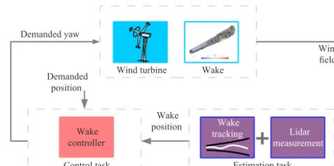
In order to enable lidar-based closed-loop wake redirection within a wind farm, two main tasks must be considered: (1) the measurement task and (2) the control task. This work focuses mainly on the measurement task but also gives a summary of a solution to the control task, which was pre-sented in Raach et al. (2016). Figure 1 presents the general concept of closed-loop wake redirection and the link between the measurement and control task.

2.1 Problem formulation for wake tracking

The main issue in the context of wake-tracking algorithms is that no clear definition exists for the wake center. Moreover, the idea of a wake center is based on time-averaged profiles of the wake behind a turbine (1 to 10 min averages). Aver-aging the flow yields a (double) Gaussian function for the velocity deficit profile in the horizontal and vertical direc-tions. From this a wake center can then be defined. However, when different methods are used to define the shape, wake center estimates may vary under the same flow conditions; see Vollmer et al. (2016). The absence of a unique wake cen-ter definition must be considered when comparing results. Furthermore, this means that, even with full-flow field infor-mation, the wake center is not a measurable quantity and de-pends on the definition. See also Doubrawa et al. (2017) and Howland et al. (2016) for a review of wake center estimation methods. The task of lidar-based wake tracking first includes a reference definition of the wake center. Then, the result of

L Wind turbine Wake

Wake controller Demanded yaw

Demanded position

Wake

position _Lidar

measurement

Estimation task

Wind ﬁeld

Control task

Wake tracking

Figure 1.The conceptual diagram of closed-loop wake redirection and its two main tasks: (1) the estimation task addressed in Sect. 5 and (2) the control task addressed in Sect. 6.

the estimation method from the lidar measurement data can be compared to the reference definition.

2.2 The estimation task

Measuring flow quantities is crucial for enabling a closed-loop controller to influence the wake properties. The task of the measurement problem is to provide the necessary quan-tities for the controller. This means using a measurement de-vice, such as a lidar, and processing the measurement data in such a way that they are useful for the controller. Since the lidar measurement principle has several limitations in provid-ing wind field information, an adequate estimation technique is used as described in Sect. 5.

2.3 The control task

The second task towards a closed-loop wake redirection is the control task. Its main challenge is to convert the esti-mated wake position information and its desired value to a demanded yaw signal. A feedback controller has to be de-signed which steers the wake center to the desired position and compensates for uncertainties in the models. Since the reaction of a change in yaw is measured with a delay due to the wake propagation time, the controller has to be designed to overcome this limitation.

(3)

s

Time in [s]

[m

]

Wake center at 226 m downstream of the turbine

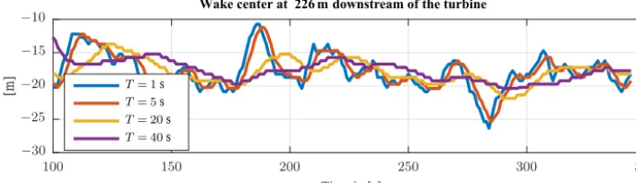
Figure 2.Time evolution of wake center (at a 1.8Ddownwind distance) when different window lengthsT are used to average the flow during the wake center calculation.

3 Reference definition and its impact on the estimation task

In this section the wake center definition is addressed through the use of simulation data, which can cover a larger area at a higher spatial and temporal resolution than measurements would be able to provide.

3.1 Wake center definition

As previously mentioned, it is first necessary to define the wake center. The minimum wind power method proposed by Vollmer et al. (2016) is adopted and modified to identify the wake center. Thus, it is defined as the downstream position at which a hypothetical turbine of identical characteristics and yaw angle would produce the least power. This yields the minimization problem

min y

2π Z

0

R+y Z

y

u(r, φ)3rdrdφ, (1)

where the position of the turbine is aty (lateral offset) and z=0 (hub-height) and the rotor area is described in the polar coordinate system (r, φ). The definition then assumes that the wake center is at (y, z).

The flow field is time averaged over different running win-dow lengths and the impact of the winwin-dow lengths is an-alyzed. The calculated wake center (at a 1.8D downwind distance) obtained with a running averaged filter with dif-ferent window lengths is presented in Fig. 2. The presented results are for a low turbulence intensity (TI=6 %) SOWFA simulation under a mean hub-height free-stream wind speed 8 m s−1. The available flow field data has a sampling fre-quency of 1 Hz and the wake center is calculated from each sample. The wake center clearly converges to a steady value with increasing averaging time T. An increased averaging time, however, slows the adjustment, e.g., to a changing wind direction or a set point change, and should be considered when choosing an averaging time.

3.2 Problem discussion of lidar-based wake tracking The problem of wake center estimation is different from other problems in lidar-based wind field reconstruction. Other model-based approaches in wind field reconstruction (e.g., estimation of the rotor-effective wind speed, or of u andvwind vector components using lidar measurements as in Schlipf et al., 2012) can first be compared to existing quan-tities. Further, the models can be used to predict line-of-sight velocities (vlos) of lidar measurements and be directly

com-pared to the real data. Therefore, the model can be used in two directions, estimating and predicting the wind field.

When the wake center is defined as in Eq. (1) the predic-tion of the wind field from a given posipredic-tion is not possible and neither is a direct comparison of line-of-sight data. Neverthe-less, the wake center position definition is used as a reference because of its robustness and simplicity.

4 A simplified wake model for wake tracking

(4)

Wind field model Lidar model Wind field characteristics Best fit wind field characteristics Optimizer

Figure 3.The general concept of model-based wind field recon-struction, in which the wind field characteristics are estimated by fitting simulated lidar measurement data (vlos,s) to measurements (vlos,m).

The general approach of wind field reconstruction from lidar data is to estimate wind field characteristics from an in-ternal model by fitting simulated lidar data to the measured ones. In Fig. 3 the basic idea of model-based wind field re-construction is shown. An optimizer is used to find the best fit for a model of the assumed wind field with the defined lidar configuration. The optimizer minimizes the square error of the modeled (simulated)vlos,s and the measuredvlos,m lidar

line-of-sight velocities and returns the estimated model pa-rameter (e.g., wake center position, wake decay, wake deficit, etc.).

In this work, a lidar and a wind field model is used. The wind field model consists of a background wind field model, which defines the ambient wind speed and its profile, and a wake model. The wake model includes the main wake effects: wake deficit, wake evolution, and wake center dis-placement. The models are presented in the following sec-tion.

4.1 Wind field model

Figure 4 shows the subparts of the wind field model: (1) the underlaying wind field and (2) the wake model.

The wind field model is described in a wind coordinate system which is denoted by the subscript W. It is rotated hor-izontally with respect to the global inertial coordinate system I and aligned with the wind direction. The wind speed vector in the W-system is transformed in the I-system by

  u v w   I =  

cosα −sinα 0 sinα cosα 0

0 0 1

    u v w   W , (2)

whereαis the horizontal rotation of the wind field. The un-derlying wind field includes the rotor effective wind speedv0

and vertical linear shearδV. It is assumed that the wind field has only aucomponent. Thus, in the W coordinate system, the underlying wind field vector at pointi with the coordi-natesxi, yi, zi

T is

Wind ﬁeld model (a) Underlaying wind ﬁeld (b) Wake effects

Figure 4.The submodels of the wind field model (in the wind coor-dinate systemW): (1) the underlaying wind field and (2) the wake model.

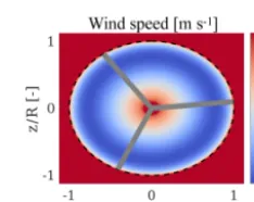
Figure 5.The initial wake deficit directly evaluated at the rotor (at 0 m downstream). The mean hub-height wind speed (8 m s−1) was removed for simplicity. No yaw misalignment is applied.

  u v w   i,W =  

v0+ziδV 0 0



, (3)

whereziis the height above the ground. This is illustrated in Fig. 4 on the left. Further, the wind field is linearly overlaid with the wake model9for theuandvcomponents yielding

  u v w   i,W =  

v0+ziδV+9u,i 9v,i

0



. (4)

In the following section, the considered wake effects are de-scribed and the wake model is presented.

4.1.1 Wake deficit and wake evolution model

The wake deficit is modeled with an initial wake deficit at the rotor disk with tip and root losses depending on the en-ergy extraction. In order to get the initial deficit, the enen-ergy extraction is mapped by applying Prandtl’s root and tip loss function0Prandtl. Applying the energy conservation

assump-tion yields

(v0+s0Prandtl)2−(1−cP)v0=0, (5)

with the power coefficient cP. Solving this equation fors

gives the initial wake deficit

(5)

Figure 6.Visualization of two wake situations within a constant wind field ofv0=16 m s−1, axial inductiona=0.15, and dissipation rate

=0.1.

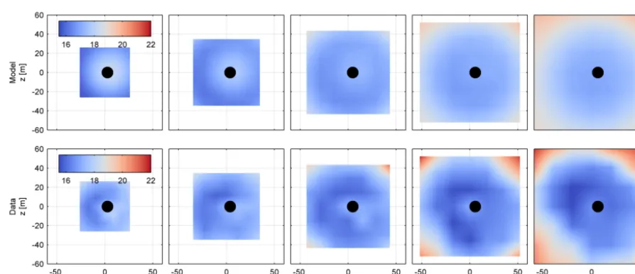
Figure 7.An example estimation step of the wake tracking. The simulated lidar measurements in the first row are compared to the measured lidar data in the second row for five downstream distances from 0.6 to 1.4D(from left to right, [0.6, 0.8, 1.0, 1.2, 1.4], looking downstream). The estimated wake center is marked with the black dot.

An example initial wake deficit9initis shown in Fig. 5.

The wake evolves as it moves away from the wind tur-bine. Energy flows in from the free stream and mixes with the wake. The Navier–Stokes equations describe the flow be-havior; however, because of the nonlinearities, using them would be a complex task. Here, an empirical model is used which models the wake recovery. However, in contrast to other wake models, the wake evolution is modeled by a Gaus-sian shape two-dimensional filter. The two-dimensional filter 4depends on the distancedbehind the wind turbine

4(d, yi, zi)=exp

y2_i +z2_i

2σ_f2(d) !

(7)

with

σf(d)= d·

2√2 log(2) (8)

andyi andzi are the grid points in distanced. With the pa-rameterthe dissipation rate can be set.

Thus, for every distance behind the rotor, the wake can be evaluated using the initial wake deficit9initand the filter

(Eq. 7). The wake deficit results from the convolution of the initial wake deficit9initwith the filter4(d, yi, zi) to

9(d, yi, zi)=4(d, yi, zi)·9init. (9)

4.1.2 Wake deflection model

The wake deflection caused by a yaw misalignmentγ is ad-ditionally modeled. The relationship is derived in the study by Jiménez et al. (2010) and was successfully used in an op-timization of the yaw angles for a simulated wind farm in Gebraad et al. (2014). The angle of the wake with respect to the main wind direction is

ξ(d, cT, γ)=

ξinit(cT, γ)

1+β_Dd

(6)

Time[s]

[m]

[

o]

w

ak

e

[-]

[s

-1]

[m s

-1]

Wake center Yaw misalignment Wake dissipation coefﬁcient

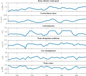
Axial induction Vertical linear shear Rotor effective wind speed

Figure 8.Time results of the wake tracking of a SOWFA simulation. The wind turbine is aligned with the mean wind direction. The lidar scanned in a 7×7 grid at five distances from 0.6 to 1.4D. The wake center is estimated at the furthest scanning distance 1.4D=176.4 m.

with the initial angle of the wake at the rotor

ξinit(cT, γ)=

1

2cos

2₍_γ_{) sin(}_γ₎_c

T (11)

and model parameterβ, which defines the sensitivity of the wake deflection to yaw and is assumed here to be known in advance. Further,cTis the thrust coefficient andDis the

ro-tor diameter. The yaw-induced deflection at the downwind positiond, according to Gebraad et al. (2014), is

δyaw(d, cT, γ)= −ξinit(cT, γ) D 30β

15

1− 1

1+2βd

D

+ξinit(cT, γ)2

1− 1

1+2βd

D 5

. (12)

The rotation is applied to the wake deficit and yields auand vcomponent of the wake model:



 9u,i 9v,i 0





W =





cosξ −sinξ 0 sinξ cosξ 0

0 0 1



 

 9i

0 0





W

. (13)

In Fig. 6 two different wake situations are shown forγ=0◦ andγ=25◦. The first is a nonyawed case and in the second case the turbine is yawed with 25◦_{. In both cases the}

underly-ing wind field has a mean hub-height free-stream wind speed ofv0=16 m s−1and no vertical shear.

5 The estimation task – model-based wake tracking

As summarized before, the estimation task tracks the wake using the presented wake model. To perform lidar-based waked tracking, a lidar model is needed. First, the lidar model is presented and then the wake-tracking approach is described. Finally, estimation results of two different cases are presented and discussed.

5.1 Lidar model

The lidar measurements can be modeled by a point measure-ment in the wind field. In the inertial coordinate system this is done by a projection of the wind vector[ui vi wi]T_I onto the normalized laser vector in theith point[xi yi zi]T_I with

focus distancefi = q

(7)

Time[s]

[m]

[

o]

w

ak

e

[-]

[s

-1]

[m s

-1]

Wake center Yaw misalignment Wake dissipation coefﬁcient

Axial induction Vertical linear shear Rotor effective wind speed

Figure 9.A second time evolution of the different estimated wind field and wake quantities. In this case, the wind turbine is misaligned with 30◦and the wake is deflected. The lidar scanned in a 7×7 grid at five distances from 0.6 to 1.4D. The wake center is estimated at the furthest scanning distance 1.4D=176.4 m.

SOWFA Lidar wake tracking

Time[s]

yL

[m

]

Wake center

100 150 200 250 300 350

30 25 20 15 10

Figure 10.Comparison between the wake center estimation (see Eq. 1) and the lidar-based wake-tracking method.

vlos,i= xi,I

fi ui,I+

yi,I fi

vi,I+ zi,I

fi

wi,I. (14)

5.2 Model-based wake tracking

As depicted in Fig. 3, the model-based wind field reconstruc-tion method estimates the model parameter by minimizing the error between measured line-of-sight wind speed vlos,m

and simulated line-of-sight wind speedvlos,s. A nonlinear

op-timization problem is formed fornmeasurement points. This yields

min p f(x)

=min

p 

 

(vlos,m,1−vlos,s,1)2 ..

.

(vlos,m,n−vlos,s,n)2 



, (15)

(8)

Table 1.The free model parameters for the wind field model which are estimated in the optimizer.

underlaying wind field wake model

v0 rotor effective wind speed cT thrust coefficient δV vertical linear shear cP power coefficient

γ turbine yaw angle

wake dissipation coefficient

Internal model Controller

Filter

Delay

τ yL

˜

yL

˜

y

yL des ∆yL γdem

Wake controller

Wake tracking

Wind turbine

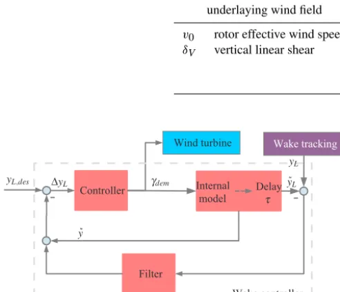
Figure 11.The general structure of the wake steering controller: the controller, a simplified wake model and the wake propagation modeled with a delay, and the filter. The controller uses the differ-enceδyL, between the predicted outputey, the measured outputyL and the desired outputyL,desto set the demanded yaw angleγdem.

5.3 Evaluation and discussion

Figure 7 confirms the applicability of the method with lidar measurement data. In the following, SOWFA (Churchfield and Lee, 2012) is used as a simulation tool. Flow snapshots of simulations of a single wind turbine are stored. The flow field is then scanned with a lidar simulator. The lidar scans with a 7×7 grid at five distances from 0.6 to 1.4D(withD=

126 m). Two different cases are analyzed. In the first case, the turbine rotor is perpendicular to the wind direction (γ=0◦) and these results are shown in Fig. 8. In the second case, the yaw misalignment is 30◦ _{so that the wake is deflected.}

The results of the wake tracking are shown in Fig. 9. In both figures the wake center is estimated at the furthest scanning distance of 1.4D=176.4 m. In both cases the method shows the ability to estimate the wake parameter and tracking its center.

As mentioned before, the wake center position needs to be calculated using a specific definition and there is no di-rect measurable representation of it. In Fig. 10 the lidar-based wake tracking is compared to the wake center estimation us-ing the definition of Eq. (1) without any filterus-ing.

6 The control task

The following closed-loop controller was first presented in Raach et al. (2016) and is recapped here. See also Raach et al. (2017), in which a H∞ controller design for

closed-loop wake redirection with defined performance margins is used. As mentioned above, the reaction of the wake to a yaw action can only be measured with a time delay. To control a delayed system, the Smith predictor approach, which is based on internal model control, has been derived and used in many applications.

The presented controller follows the idea of internal model control in which the difference between the actual system output and a predicted output is used within the controller to regulate the system. Therefore, a model is necessary for de-scribing the wake effects in a simplified but sufficient way. It consists of a proportional-integral (PI) controller. Further, an internal model is used which approximates the real system behavior. The wake propagation which exists because the wake flow has to evolve until it reaches the measurement lo-cation of the lidar system is modeled using a time delay. The delay timeτ varies with respect to the mean wind speed. Fi-nally, a filter is needed to cancel out controller actions which can not be observed because of the time difference between control action and measurement location. Figure 11 shows the general concept of the controller.

6.1 Internal wake model of the controller

As depicted in Fig. 11, the wake controller needs an internal model to predict the reaction of the wake to the demanded yaw angle. The internal wake model includes the yaw actu-ator and the gain between the yaw and the wake deflection. For the wake model the assumptions of a constantcTis made.

Altogether, this yields an internal controller model9eof the reality9:

e 9:

¨

γ+2dωγ˙+ω2γ=ω2γdem

ey = δyaw(dLidar, cT,const, γ)

, (16)

withγdembeing the demanded yaw angle anddLidarthe

dis-tance to the measurement location. Equation (16), line 1 is the yaw actuator dynamic and Eq. (16), line 2 the wake de-flection model.

There is a time delay because the wake first needs to evolve to the measurement location:

eyL(t)=ey(t−τ). (17)

(9)

[Hz]

[

o]

[d

B

]

Phase Magnitude

Figure 12.Bode analysis of the designed controllerK.

[Hz]

[d

B

]

[d

B

]

[d

B

]

Controller sensitivity Complementary sensitivity

Sensitivity

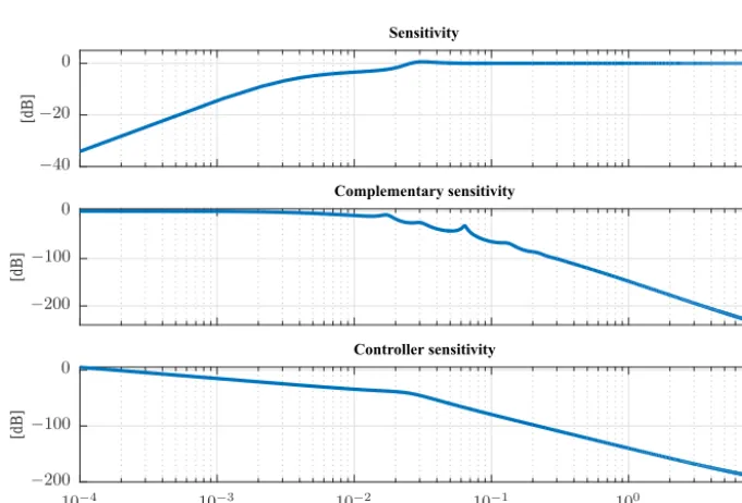
Figure 13.SensitivityS, complementary sensitivityT, and controller sensitivityUanalysis of the closed-loop system.

6.2 Controller design

The primal goal of the wake controller is to steer the wake center to a desired point in a defined distance by yawing the wind turbine. As mentioned, this is done using a Smith predictor, which uses an internal model to predict the out-put reaction. Then the predicted wake center position and the filtered error between predicted and measured wake center position is fed back to the controller.

6.2.1 Controller

A standard PI controller is used. It is designed such that the closed-loop performance with the internal model (Eq. 16) meets a phase margin of 60◦ and a closed-loop bandwidth

ofωCL=₂1_τ. This yields a controller of the form

u=Kp

1yL+

1 Ti

Z

1yLdt, (18)

with the proportional gainKp, the time constantTi, and the error between desired and actual wake center position1yL.

6.2.2 Filter

(10)

the cutoff frequency of the butterworth low-pass filter is set toωfilter=₈π_τ.

6.3 Evaluation and discussion

In the following the wake controller is analyzed. Further, the sensitivity, the complementary sensitivity, and the controller sensitivity of the closed-loop system are assessed. Consid-ering Skogestad and Postlethwaite (2005), the sensitivity gives the closed-loop transfer function from the output dis-turbance to the output while the complementary sensitivity is the closed-loop transfer function from the reference to the output. The controller sensitivity gives the closed-loop trans-fer function from the output disturbance to the controller. For more details and a description on controller design and anal-ysis, we refer to Skogestad and Postlethwaite (2005).

6.3.1 Controller analysis

In the following, the transfer function of the wake controller is assessed. As shown in Fig. 11 the wake controller consists of the internal controllerC, an internal model9e, the time delay approximationW, and the filterF. Having merged all parts the wake controllerKis

K= F

(1+C 9(1−F W)). (19)

Figure 12 shows the bode analysis of the wake controller K. The controller shows integration behavior, starting with

−90◦phase.

6.3.2 Closed-loop analysis

To perform closed-loop analysis the internal controller model

e

9 is transformed to Laplacian space, yielding the plantG. Then, the sensitivityS, the complementary sensitivityT, and the controller sensitivityUthat are

S= 1

1+GK (20)

T = GK

1+GK (21)

U= K

1+GK, (22)

with the controllerKare assessed and shown in Fig. 13. The sensitivity shows a disturbance attenuation up to the con-troller bandwidthωCL=0.02 Hz. Further, the controller

sen-sitivity has low gain for high frequencies. This means the controller does not react to high-frequency disturbances.

7 Conclusions

This paper first introduces a method which uses lidar mea-surements to estimate wind field parameters and enables

tracking of the wake center position. Second, a controller is presented which uses this information to redirect the wake to a desired position. In two different cases using simulated li-dar measurements of SOWFA simulations, the wake tracking shows promising results in estimating the wake center. The difficulty in wake center position definition is elaborated. A definition is used and the wake-tracking results are compared to it. The challenges of a lidar-based wake redirection con-trol problem are discussed and an appropriate concon-troller is designed to meet the desired requirements. This leads to the next step, towards closed-loop wake redirection in a high-fidelity simulation tool.

The presented framework of lidar-based closed-loop wake steering offers new possibilities for wind farm control. In the future, a balance between measuring the near wake, which will result in a higher controller bandwidth, and the far wake, which will give more reliable information on the wake direc-tion, needs to be found. In a next step, it will be implemented and tested in a high-fidelity simulation tool and tested in real time. For the control problem, robust controllers will be in-vestigated. Dynamic estimation techniques as well as other wake estimation models will be used for comparing the abil-ity of tracking the wake and finding the most suitable ap-proach for this task.

Data availability. The SOWFA data used in this work have been provided by the National Reneawable Energy Laboratory (NREL) and is publicly available at http://wind.nrel.gov/public/ssc/.

Competing interests. The authors declare that they have no con-flict of interest.

Acknowledgements. The authors would like to acknowledge the CL-Windcon project which has received funding from the Eu-ropean Union’s Horizon 2020 research and innovation programme under grant agreement No 727477. Further, we would like to thank Pieter Gebraad and Paul Fleming for fruitful discussions and providing the SOWFA data set.

Edited by: C. L. Bottasso

Reviewed by: two anonymous referees

References

Boersma, S., Doekemeijer, B., Gebraad, P., Fleming, P., Annoni, J., Scholbrock, A., Frederik, J., and van Wingerden, J.-W.: A Tuto-rial on Control-Oriented Modeling and Control of Wind Farms, in: Proceedings of the American Control Conference (ACC), Seattle, USA, 2017.

(11)

Churchfield, M. and Lee, S.: NWTC design codes-SOWFA, avail-able at: http://wind.nrel.gov/designcodes/simulators/SOWFA (last access: 15 May 2017), 2012.

Doubrawa, P., Barthelmie, R. J., Wang, H., and Churchfield, M. J.: A stochastic wind turbine wake model based on new metrics for wake characterization, Wind Energy, 20, 449–463, doi:10.1002/we.2015, 2017.

Fleming, P., Gebraad, P. M., Lee, S., Wingerden, J.-W., Johnson, K., Churchfield, M., Michalakes, J., Spalart, P., and Moriarty, P.: Simulation comparison of wake mitigation control strategies for a two-turbine case, Wind Energy, 18, 2135–2143, 2014a. Fleming, P. A., Gebraad, P. M., Lee, S., van Wingerden, J.-W.,

John-son, K., Churchfield, M., Michalakes, J., Spalart, P., and Mori-arty, P.: Evaluating techniques for redirecting turbine wakes us-ing SOWFA, Renew. Energ., 70, 211–218, 2014b.

Gebraad, P. M. O., Teeuwisse, F. W., van Wingerden, J., Fleming, P., Ruben, S. D., Marden, J. R., and Pao, L. Y.: Wind plant power optimization through yaw control using a parametric model for wake effects – a CFD simulation study, Wind Energy, 19, 95– 114, doi:10.1002/we.1822, 2014.

Howland, M. F., Bossuyt, J., Martinez-Tossas, L. A., Meyers, J., and Meneveau, C.: Wake Structure of Wind Turbines in Yaw un-der Uniform Inflow Conditions, available at: http://arxiv.org/abs/ 1603.06632 (last access: 15 May 2017), 2016.

Jiménez, Á., Crespo, A., and Migoya, E.: Application of a LES tech-nique to characterize the wake deflection of a wind turbine in yaw, Wind Energy, 13, 559–572, 2010.

Lundquist, J. K., Churchfield, M. J., Lee, S., and Clifton, A.: Quan-tifying error of lidar and sodar Doppler beam swinging measure-ments of wind turbine wakes using computational fluid dynam-ics, Atmos. Meas. Tech., 8, 907–920, doi:10.5194/amt-8-907-2015, 2015.

Raach, S., Schlipf, D., Haizmann, F., and Cheng, P. W.: Three Di-mensional Dynamic Model Based Wind Field Reconstruction from LiDAR Data, in: Journal of Physics: Conference Series: The Science of Making Torque From Wind, Vol. 524, Copen-hagen, Denmark, 2014.

Raach, S., Schlipf, D., Borisade, F., and Cheng, P. W.: Wake redi-recting using feedback control to improve the power output of wind farms, in: Proceedings of the American Control Conference (ACC), Boston, USA, 2016.

Raach, S., van Wingerden, J.-W., Boersma, S., Schlipf, D., and Cheng, P. W.: Hinf controller design for closed-loop wake redi-rection, in: Proceedings of the American Control Conference (ACC), Seattle, USA, 2017.

Schlipf, D., Rettenmeier, A., Haizmann, F., Hofsäß, M., Courtney, M., and Cheng, P. W.: Model Based Wind Vector Field Recon-struction from Lidar Data, in: Proceedings of the German Wind Energy Conference DEWEK, Bremen, Germany, 2012. Skogestad, S. and Postlethwaite, I.: Multivariable Feedback

Con-trol: Analysis and Design, John Wiley & Sons, New York, USA, 2005.