www.geosci-instrum-method-data-syst.net/6/149/2017/ doi:10.5194/gi-6-149-2017
© Author(s) 2017. CC Attribution 3.0 License.
Soil salinity mapping and hydrological drought indices assessment
in arid environments based on remote sensing techniques
Mohamed Elhag and Jarbou A. Bahrawi
Department of Hydrology and Water Resources Management, Faculty of Meteorology, Environment & Arid Land Agriculture, King Abdulaziz University, Jeddah 21589, Saudi Arabia
Correspondence to:Mohamed Elhag ([email protected])
Received: 19 November 2016 – Discussion started: 8 December 2016
Revised: 14 February 2017 – Accepted: 1 March 2017 – Published: 15 March 2017
Abstract. Vegetation indices are mostly described as crop water derivatives. The normalized difference vegetation in-dex (NDVI) is one of the oldest remote sensing applica-tions that is widely used to evaluate crop vigor directly and crop water relationships indirectly. Recently, several NDVI derivatives were exclusively used to assess crop water rela-tionships. Four hydrological drought indices are examined in the current research study. The water supply vegetation in-dex (WSVI), the soil-adjusted vegetation inin-dex (SAVI), the moisture stress index (MSI) and the normalized difference infrared index (NDII) are implemented in the current study as an indirect tool to map the effect of different soil salinity levels on crop water stress in arid environments. In arid en-vironments, such as Saudi Arabia, water resources are under pressure, especially groundwater levels. Groundwater wells are rapidly depleted due to the heavy abstraction of the re-served water. Heavy abstractions of groundwater, which ex-ceed crop water requirements in most of the cases, are pow-ered by high evaporation rates in the designated study area because of the long days of extremely hot summer. Landsat 8 OLI data were extensively used in the current research to ob-tain several vegetation indices in response to soil salinity in Wadi ad-Dawasir. Principal component analyses (PCA) and artificial neural network (ANN) analyses are complementary tools used to understand the regression pattern of the hydro-logical drought indices in the designated study area.
1 Introduction
Remote sensing data are considered to be a convenient source to perform several vegetation indices in either simple or com-plicated band ratio combinations. Satellite images offer a large amount of data that could be analyzed, processed and stored to better understand several vegetation indices based on the type of the satellite sensor used (Govaerts et al., 1999; Pinty et al., 2009). Hypothetical backgrounds have been im-plemented to improve and enhance the optimization of par-ticular satellite sensors to support certain vegetation indices (Verstraete et al., 1996; Gobron et al., 2000; Psilovikos and Elhag, 2013).
Spectral vegetation indices are mathematical combina-tions of different spectral bands mostly in the visible and near-infrared regions of the electromagnetic spectrum. Vege-tation activities can be measured comprehensively through semi-analytical methods of spectral band ratios that have been extensively used to detect not only seasonal variability of the vegetation cover but also local scale spatial variability (Broge and Mortensen, 2002; Xiao et al., 2002).
Soil parameter variation tends to draw a line on a plenary scattergram. Nevertheless, this line, used as a reference point and known as a “soil line” in vegetation studies, involved both red and infrared spectral bands (Colombo et al., 2003; Elhag, 2014a, b). The utilization of vegetation indices has always been challenged by a major difficulty, which is the minimization of soil component interferences and sensitiv-ity maximization of atmospheric variations (Qi et al., 1994; Leprieur et al., 2000). The atmospherically resistant vegeta-tion index (ARVI), developed by Kaufman and Tanré (1992), and the global environmental monitoring index (GEMI), de-veloped by Pinty and Verstraete (1992), are the less sensitive vegetation indices to atmospheric variation. Additionally, Qi et al. (1994) reported that the GEMI is soil noise sensitive. The higher noise sensitivity of GEMI has completely dis-abled the index and classified it as inadequate for arid re-gions.
Implementations of vegetation indices varied, from a local leaf scale to a continental vegetation scale. Moreover, cer-tain indices tend to be site and/or species specific (Clevers, 1989; Elhag, 2014a), and they cannot be applied to differ-ent species or differdiffer-ent leaf structures and canopy geometry (Xiao et al., 2002). The scholarly work of Kerr and Ostro-vsky (2003), Pettorelli et al. (2005), Huete et al. (2008) and Elhag (2014b) reported that several vegetation indices were used to estimate different vegetation parameters extensively, including the leaf area index (LAI), the fractional vegetation cover (FC), the crop water stress index (CWSI), the drought severity index (DSI) and the water supply vegetation index (WSVI).
Soil salinization is a dynamic process that basically arises when an excess of irrigational water is frequently used in the drainage capacity of the fields (Wardlow and Egbert, 2010). Implementations of remote sensing techniques in soil salin-ity mapping achieved comprehensive results on the regional scale (Montandon and Small, 2008). The brightness index (BI), the normalized difference salinity index (NDSI) and the salinity index (SI) are widely distinguished in soil salinity mapping in an arid environment (Douaoui et al., 2006; Jia-paer et al., 2011). The current research aims to evaluate the suitability of different vegetation indices for a different level of remotely sensed soil salinity contrasting to crop water re-lationship in Wadi ad-Dawasir.
2 Materials and methods 2.1 Study area
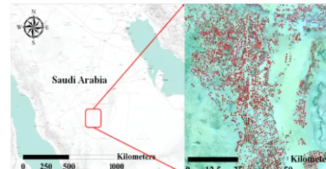
The study area,the Wadi ad-Dawasir town, is located in the plateau of Najd at 44◦430lat and 20◦290long, about 300 km south of the capital city, Riyadh. The study area illustrated in Fig. 1 is comprised of gravelly tableland disconnected by insignificant sandy oases and isolated mountain bundles. Across the Arabian Peninsula, as a whole, the tableland
Figure 1.Location of the study area (Elhag, 2016).
slopes toward the east from an elevation of 1360 m in the west to 750 m at its easternmost limit. Wadi ad-Dawasir and Wadi al-Rummah, which are the most important patterns of the ancient riverbeds, remain in the study area. The Wadi ad-Dawasir and Najran regions are the major irrigation wa-ter abstractors from the Al-Wajid aquifer. Agriculture in the Wadi ad-Dawasir area consists of technically highly devel-oped farm enterprises that operate with modern pivot irri-gation systems. The size of center pivot ranges from 30 to 60 ha, with farms managing hundreds of them with the cor-responding number of wells. The main crop grown in winter is wheat and occasionally potatoes, tomatoes or melons. All-year fodder consists of alfalfa, which is cut up to 10 times a year for food. Typical summer crops for fodder are sorghum and Rhodes grass, which is perennial but dormant in win-ter. The shallow alluvial aquifers could not sustain the high groundwater abstraction rates for a long time and groundwa-ter level declined dramatically in most areas. Meteorological features of the area are speckled. Five elements of meteorol-ogy are constantly recorded through a fixed weather station located within the study area. Temperature varies from a min-imum of 6◦C to a maximum of 43◦C. Relative humidity is mostly stable at 24 %. Solar radiation of average sunrise du-ration is generally 11 h day−1. Average wind speed is closer to 13 km h−1and may reach up to 46 km h−1in thunderstorm incidents. Finally, mean annual rainfall is about 37.6 mm (Al-Zahrani and Baig, 2011).
2.2 Methodological framework
2.3 Estimation of vegetation indices
2.3.1 Water supply vegetation index (WSVI) The water supply vegetation index is calculated by
WSVI=NDVI/Ts, (1)
whereTs is the estimated brightness temperature channel or related remote sensing imagery, and NDVI is the normal-ized difference vegetation index. The smaller this index is, the more severe the drought is.
2.3.2 Soil-adjusted vegetation index (SAVI) The soil-adjusted vegetation index is calculated by SAVI= (NIR−R)
(NIR+R)·(1+L), (2)
where NIR is the near-infrared band, R is the red band and
L is the is the soil brightness correction factor, commonly
L=0.5 (Huete, 1988).
2.3.3 Moisture stress index (MSI) The moisture stress index is calculated by MSI=SWIR1
NIR , (3)
where SWIR1is the short-wave infrared band 1. 2.3.4 Normalized difference infrared index (NDII) The normalized difference infrared index is calculated by NDII=(NIR−SWIR1)
(NIR+SWIR1)
. (4)
2.4 Estimation of soil salinity index
Soil salinity indices are principally adjusted to detect salt mineral in soils based on the different responses of salty soils to various spectral bands. The following equation to map soil salinity was used following Elhag (2016).
SI=(G×R)/B, (5)
where B is the blue band, G is the green band and R is the red band.
2.5 Regression analyses
The purpose of the regression analyses is to envisage the re-gression potentials between the soil salinity index from one side and the rest of the hydrological drought indices from the other side. The principal component analyses and artifi-cial neural network (ANN) analyses were the implemented
approaches. The PCA is used to transform a set of likely cor-related with unlikely corcor-related variables. The principal com-ponents number is less than or equal to the variables’ origi-nal number. Following Lorenz (1956), the PCA fundamental equations are described as follows.
First, vectorW(1)has to be calculated as follows:
w(1)=arg max
kwk=1 nX
i(t1) 2 (i)
o
=arg max
kwk=1 nX
i(xi ·w)
2o. (6)
The matrix form of the above equation gives the following:
w(1)=arg max
kwk=1 n
kXwk2o
=arg max
kwk=1 n
wTXTXw
o
. (7)
W(1)has to be calculated as follows:
w(1)=arg max
wTXTXw
wTw
. (8)
The resultingw(1)suggests that the first component of a data vector,x(i), can then be expressed as a score oft1(i)=x(i)·
w(1)in the transformed co-ordinates or as the corresponding vector in the original variables,{x(i)·w(1)}w(1).
The neural network regression model is written as
Y=α+X
hwhφh
αh+
Xp i=1wihXi
, (9)
whereY=E(Y|X).This neural network model has one hid-den layer, but it is possible to have additional hidhid-den layers.
The φ (z) function used is hyperbolic tangent activation
function. It is used for logistic activation for the hidden lay-ers.
φ (z)=tanh (z)=1−e
−2z
1+e−2z. (10)
Significantly, the final output should be stochastically linear, with no prediction limitations being between 0 and 1. A sim-ple diagram of a skip-layer neural network is illustrated in Fig. 2. The equation for the skip-layer neural network for re-gression is shown below.
Y=α+Xp
i=1βiXi +
X
hwhφh
αh+
Xp
i=1wihXi
. (11)
Figure 2.Artificial neural network scheme with one hidden layer and three nodes.
reasons. RMSE can be computed as follows:
RMSE=
s 1
T0
XT0
t=1 y1−ý1 2
, (12)
where t is the time index and yˆt and yt are the simulated and measured values. Principally, the higher value ofRand smaller values of RMSE ensure the better performance of the model.
3 Results and discussion
The realization of the hydrological drought indices was exer-cised after a comprehensive remote sensing data correction. Basically, atmospheric correction and spatial enhancement were practiced utilizing Landsat 8 OLI data acquired over the designated study area. The four hydrological drought indices were shown in Figs. 3 to 6. Stochastic algorithms of WSVI and SAVI mapping (Figs. 3 and 4) showed spatial coherence with higher drought indices’ values within the agricultural area rather than the surrounding area (Ceccato et al., 2001; Daughtry et al., 2004).
On the contrary, MSI functioned as a deterministic drought index, it was nearly unaffected by changing water content. Conducted results showed two classes of stresses: stressed and no stress. The no stress class was located within the agri-cultural area, and the stressed area was represented along the agricultural peripheral areas (Fig. 5), where higher values in-dicate greater water stress and less water content. This could be explained rationally by the presence of irrigational sprin-kles (Hunt Jr. and Rock, 1989; Ceccato et al., 2001). NDII is also a stochastic algorithm and was used in the current re-search due to the higher sensitivity of the infrared band to detect changes in water content of plant canopies (Hardisky et al., 1983). The spatial distribution of NDII (Fig. 6) was mapped accordingly with WSVI and SAVI indices, in which higher NDII values meant higher water content (Jackson et al., 2004). There are several algorithms to map soil salin-ity based on utilization of different remote sensing data and
Figure 3.Water supply vegetation index (WSVI) thematic map over the study area.
different ecological systems. An adequate NDSI algorithm was carried out according to Elhag (2016) findings in arid ecosystems. In Fig. 7, NDSI showed spatial variation, espe-cially within the new agricultural expansion at the southwest-ern part of the study area. The sprinkle movement drove the salt accumulation to be located at the peripherally of the agri-cultural areas (Lunetta et al., 2006; Konukcu et al., 2006).
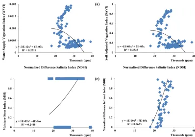
Further statistical analyses were carried out to construe the correspondences between salted soils and different horologi-cal drought indices. The regression analysis demonstrated in Fig. 8 showed that salinity increases with lower WSVI and SAVI (Fig. 8a, b), which is explained by the salt accumula-tion in soils in parts per million (ppm). Under salinity stress conditions, there is not enough available water in soils for proper vegetation growth (Lunetta et al., 2006; Yang et al., 2011).
Generally, MSI values (Fig. 8c) are high in the study area because of the excess irrigation regime adopted to over-come the high evaporation rates (Elhag and Bahrawi, 2014; Elhag, 2016). Excess irrigation regimes in poor-drain soils lead to waterlogging problems and salts accumulation (El-hag, 2016).
Due to NDII’s higher sensitivity to water, NDII values in-crease with higher NDSI values. Salts accumulation caused by excessive irrigation is the driving force behind the propor-tional increment of NDII values in conjunction with NDSI values as demonstrated in Fig. 8d (Jackson et al., 2004; Shi et al., 2015).
de-Figure 4.Soil-adjusted vegetation index (SAVI) thematic map over the study area.
Figure 5.Moisture stress index (MSI) thematic map over the study area.
composition was also demonstrated. WSVI and SAVI were grouped together. Additionally, NDII and MSI were individ-ually plotted against the former indices.
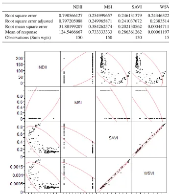
Similar results conducted from the scatterplot matrix and the accompanying correlation matrix are shown in Fig. 10 and Table 1. A high correlation is distinguished between WSVI and SAVI, while a negative correlation is noted be-tween WSVI and SAVI from one side and MSI and NDII from the other side.
Figure 6.Normalized difference infrared index (NDII) thematic map over the study area.
Figure 7.Normalized difference salinity index (NDSI) thematic map over the study area.
y = -1E-09x2 + 5E-05x
R² = 0.2338 0 0.2 0.4 0.6 0.8 1
0 10 20 30 40
So il A dj us ted V eg et at io n In dex ( SAV I)
Normalized Difference Salinity Index (NDSI) Thousands (ppm)
y = 1E-09x2 - 4E-06x
R² = 0.2448 0 0.2 0.4 0.6 0.8 1
0 10 20 30 40
Normalized Difference Salinity Index (NDSI) Thousands (ppm)
y = 4E-09x2 - 7E-05x
R² = 0.7633 0 0.2 0.4 0.6 0.8 1
0 10 20 30 40
N or m al iz ed D iffe re nc e In fr ar ed I nd ex (N D II )
Normalized Difference Salinity Index (NDSI) Thousands (ppm) y = -3E-12x2 + 1E-07x
R² = 0.2318 0
0.0005 0.001 0.0015 0.002
0 10 20 30 40
W at er S u pp ly V eg et at io n I n de x (W S V I)
Normalized Difference Salinity Index (NDSI) Thousands (ppm)
(a) (b)
(c) (d)
Moisture S tess In de x (MSI )
Figure 8.Regression analyses of NDSI (ppm) against horological drought indices.
Figure 9.Principal component analysis.
Table 1.Correlation matrix.
NDII MSI SAVI WSVI
NDII 1 0.7182080406 −0.708975719 −0.703572559 MSI 1 −0.888156103 −0.88249756 SAVI 1 0.9977255509
WSVI 1
combinations of the four hydrological drought indices were not correlated.
Table 2.Regression analysis.
NDII MSI SAVI WSVI
Root square error 0.798566127 0.254999657 0.246131379 0.243463225
Root square error adjusted 0.797205088 0.249965871 0.241037672 0.23835149
Root mean square error 31.88199207 0.384262574 0.202130562 0.000447112
Mean of response 124.5466667 0.733333333 0.286361262 0.000611978
Observations (Sum wgts) 150 150 150 150
Figure 10.Scatterplot correlation matrix.
WSVI. MSI failed to fit NDSI values comprehensively, like the former hydrological drought indices (Jones and Marshall, 1992; Jiapaer et al., 2011).
4 Conclusions
The findings of the current research emphasize the im-portance of the hydrological drought indices to envisage the adverse effects of salts accumulation in poorly drained soils similar to the study area under investigation. The soils of Wadi ad-Dawasir are poorly drained and still under heavy pressure of heavy irrigation schemes to overcome the high evaporation rates. Therefore, the implemented irrigation schemes should be adjusted for better natural resources man-agement. Remote Sensing techniques were satisfactorily im-plemented and interpreted in terms of soil salinity mapping
in consort with hydrological drought indices. The normalized difference infrared index was statistically proven to be the profound normalized difference salinity index, followed by soil-adjusted vegetation index and water supply vegetation index, respectively. The principal component analyses and artificial neural network analyses are complementary tools used to understand the regression patterns of the hydrologi-cal drought indices in the designated study area. Further work needs to be considered towards the restrictiveness of the dras-tic effect of salts accumulation within the study area.
Table 3.Spearman’s correlation.
Variable By variable Correlation Count Lower 95 % Upper 95 % Significance probability
MSI NDII 0.7182 150 0.6305 0.7878 *
SAVI NDII −0.7090 150 −0.7805 −0.6191 NS
SAVI MSI −0.8882 150 −0.9178 −0.8487 NS
WSVI NDII −0.7036 150 −0.7763 −0.6124 NS
WSVI MSI −0.8825 150 −0.9136 −0.8412 NS
WSVI SAVI 0.9977 150 0.9969 0.9984 **
Note that * is significant, ** is highly significant and NS is non-significant.
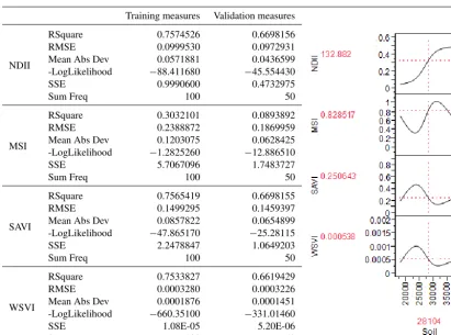
Table 4.Neural network analysis.
Training measures Validation measures
NDII
RSquare 0.7574526 0.6698156
Table 4. Neural Network Analysis. 545
Training Measures Validation Measures
N
D
II
RSquare 0.7574526 0.6698156
RMSE 0.0999530 0.0972931
Mean Abs Dev 0.0571881 0.0436599
-LogLikelihood -88.411680 -45.554430
SSE 0.9990600 0.4732975
Sum Freq 100 50
M
SI
RSquare 0.3032101 0.0893892
RMSE 0.2388872 0.1869959
Mean Abs Dev 0.1203075 0.0628425
-LogLikelihood -1.2825260 -12.886510
SSE 5.7067096 1.7483727
Sum Freq 100 50
SA
V
I
RSquare 0.7565419 0.6698155
RMSE 0.1499295 0.1459397
Mean Abs Dev 0.0857822 0.0654899
-LogLikelihood -47.865170 -25.28115
SSE 2.2478847 1.0649203
Sum Freq 100 50
W
S
V
I
RSquare 0.7533827 0.6619429
RMSE 0.0003280 0.0003226
Mean Abs Dev 0.0001876 0.0001451
-LogLikelihood -660.35100 -331.01460
SSE 1.08E-05 5.20E-06
Sum Freq 100 50
546
547
548
RMSE 0.0999530 0.0972931
Mean Abs Dev 0.0571881 0.0436599
-LogLikelihood −88.411680 −45.554430
SSE 0.9990600 0.4732975
Sum Freq 100 50
MSI
RSquare 0.3032101 0.0893892
RMSE 0.2388872 0.1869959
Mean Abs Dev 0.1203075 0.0628425
-LogLikelihood −1.2825260 −12.886510
SSE 5.7067096 1.7483727
Sum Freq 100 50
SAVI
RSquare 0.7565419 0.6698155
RMSE 0.1499295 0.1459397
Mean Abs Dev 0.0857822 0.0654899
-LogLikelihood −47.865170 −25.28115
SSE 2.2478847 1.0649203
Sum Freq 100 50
WSVI
RSquare 0.7533827 0.6619429
RMSE 0.0003280 0.0003226
Mean Abs Dev 0.0001876 0.0001451
-LogLikelihood −660.35100 −331.01460
SSE 1.08E-05 5.20E-06
Sum Freq 100 50
RSquare=root square error and RMSE=root mean square error.
Competing interests. The authors declare that they have no conflict of interest.
Acknowledgements. This work was supported by the Deanship of Scientific Research (DSR), King Abdulaziz University, Jeddah, under grant No. 155-36-1437-D. The authors, therefore, gratefully acknowledge the DSR’s technical and financial support.
Edited by: L. Eppelbaum
Reviewed by: S. Boteva and N. Yilmaz
References
Al-Zahrani, K. H. and Baig, M. B.: Water in the Kingdom of Saudi Arabia: Sustainable Management Options, J. Anim. Plant Sci., 21, 601–604, 2011.
Boegh, E., Soegaard, H., Broge, N., Hasager, C. B., Jensen, N. O., Schelde, K., and Thomsen, A.: Airborne multispectral data for quantifying leaf area index, nitrogen concentration, and photo-synthetic efficiency in agriculture, Remote Sens. Environ., 81, 179–193, 2002.
Bouman B. A. M. and Tuong, T. P.: Field water management to save water and increase its productivity in irrigated rice, Agr. Water Manage., 49, 11–30, 2001.
Broge, N. H. and Mortensen, J. V.: Deriving green crop area index and canopy chlorophyll density of winter wheat from spectral reflectance data, Remote Sens. Environ., 81, 45–57, 2002. Ceccato, P., Flasse, S., Tarantola, S., Jacquemoud, S., and Gregoire,
J. M.: Detecting vegetation leaf water content using reflectance in the optical domain, Remote Sens. Environ., 77, 22–33, 2001. Clevers, J. G. P. W.: The application of a weighted infrared-red
veg-etation index for estimating leaf-area index by correcting for soil-moisture, Remote Sens. Environ., 29, 25–37, 1989.
Colombo, R., Bellingeri, D., Fasolini, D., and Marino, C. M.: Re-trieval of leaf area index in different vegetation types using high resolution satellite data, Remote Sens. Environ., 86, 120–131, 2003.
Curran, P. J.: Estimating green LAI from multispectral aerial-photography, Photogramm. Eng. Rem. S., 49, 1709–1720, 1983a. Curran, P. J.: Multispectral remote-sensing for the estimation of green leaf area index, Philos. T. Roy. Soc. A, 309, 257–270, 1983b.
Daughtry, C. S. T., Hunt Jr., E. R., and McMurtrey III, J. E.: As-sessing crop residue cover using shortwave infrared reflectance, Remote Sens. Environ., 90, 126–134, 2004.
Douaoui, A. K., Hervé, N., and Walter, C.: Detecting salinity haz-ards within a semiarid context by means of combining soil and remote sensing data, Geodema, 134, 217–230, 2006.
Elhag, M.: Evaluation of Different Soil Salinity Mapping Using Remote Sensing Techniques in Arid Ecosystems, Saudi Arabia, Journal of Sensors, 2016, 96175–96175, 2016.
Elhag, M.: Remotely Sensed Vegetation Indices and Spatial Deci-sion Support System for Better Water consumption Regime in the Nile Delta. A Case Study for Rice Cultivation Suitability Map, Life Science Journal, 11, 201–209, 2014a.
Elhag, M.: Sensitivity Analysis Assessment of Remotely Based Vegetation Indices to Improve Water Resources Management, Environment Development and Sustainability, 16, 1209–1222, 2014b.
Elhag, M. and Bahrawi, J.: Conservational Use of Remote Sensing Techniques for a Novel Rainwater Harvesting in Arid Environ-ment, Environ. Earth Sci., 72, 4995–5005, 2014.
Gobron, N., Pinty, B., Verstraete, M. M., and Widlowski, J. L.: Advanced vegetation indices optimized for up-coming sensors: Design, performance, and applications, IEEE T. Geosci. Remote Sens., 38, 2489–2505, 2000.
Govaerts, Y. M., Verstraete, M. M., Pinty, B., and Gobron, N.: De-signing optimal spectral indices: A feasibility and proof of con-cept study, Int. J. Remote Sens., 20, 1853–1873, 1999.
Hardisky, M., Klemas, V., and Smart, R.: The influence of soil salin-ity, growth form, and leaf moisture on the spectral radiance of Spartina alternifloracanopies, Photogramm. Eng. Rem. S., 49, 77–83, 1983.
Huete, A. R.: A soil-adjusted vegetation index (SAVI), Remote Sens. Environ., 25, 295–309, 1988.
Huete, A., Didan, K., van Leeuwen, W., Miura, T., and Glenn, E.: MODIS vegetation indices, in: Land Remote Sensing and Global Environmental Change: NASA’s Earth Observing System and the Science of ASTER and MODIS, 125–146, 2008.
Hunt Jr., E. R. and Rock, B. N:. Detection of changes in leaf wa-ter content using near- and middle infrared reflectances, Remote Sens. Environ., 30, 43–54, 1989.
Jackson, T. J., Chen, D. Y., Cosh, M., Li, F. Q., Anderson, M., Walthall, C., Doriaswamya, P., and Hunt Jr., R. E.: Vegetation water content mapping using Landsat data derived normalized difference water index for corn and soybeans, Remote Sens. En-viro., 92, 475–482, 2004.
Jiang, B.: Head/Tail Breaks: A New Classification Scheme for Data with a Heavy-Tailed Distribution, Prof. Geogr., 65, 482–494, 2013.
Jiapaer, G., Chen, X. and Bao, A. M.: A comparison of methods for estimating fractional vegetation cover in arid regions, Agr. Forest Meteorol., 151, 1698–1710, 2011.
Jones, R. and Marshall, G.: Land salinization, waterlogging and the agricultural benefits of a surface drainage scheme in Benerembah irrigation district. Review of Marketing and Agricultural Eco-nomics, 60, 173–189, 1992.
Kaufman, Y. J. and Tanré, D.: Atmospherically resistant vegetation index (ARVI) for EOS-MODIS, Transactions on Geoscience and Remote Sensing, 30, 261–270, 1992.
Kerr, J. and Ostrovsky, M.: From space to species: ecological ap-plications for remote sensing, Trends Ecol. Evol., 18, 299–305, 2003.
Konukcu, F., Gowing, J. W., and Rose, D. A.: Dry drainage: a sus-tainable solution to waterlogging and salinity problems in irriga-tion areas?, Agr. Water Manage., 83, 1–12, 2006.
Leprieur, C., Kerr, Y. H., Mastorchio, S., and Meunier, J. C.: Moni-toring vegetation cover across semi-arid regions: Comparison of remote observations from various scales, Int. J. Remote Sens., 21, 281–300, 2000.
Lorenz, E. N.: Empirical orthogonal functions and statistical weather prediction, MIT Department of Meteorology, Statistical Forecast Project Rep. 1, 49 pp., Available from Dept. of Meteo-rology, MIT, Massachusetts Ave., Cambridge, MA 02139, 1956. Lunetta, R. S., Knight, J. F., Ediriwickrema, J., Lyon, J. G., and Worthy, L. D.: Land-cover change detection using multi-temporal MODIS NDVI data, Remote Sens. Environ., 105, 142– 154, 2006.
Montandon, L. M. and Small, E. E.: The impact of soil reflectance on the quantification of the green vegetation fraction from NDVI, Remote Sens. Environ., 112, 1835–1845, 2008.
Moulin, S. and Guerif, M.: Impacts of model parameter uncer-tainties on crop reflectance estimates: A regional case study on wheat, Int. J. Remote Sens., 20, 213–218, 1999.
Pettorelli, N., Vik, J., Mysterud, A., Gaillard, J., Tucker, C., and Stenseth, N.: Using the satellite-derived NDVI to assess ecolog-ical responses to environmental change, Trends Ecol. Evol., 20, 503–510, 2005.
Pinty, B. and Verstraete, M. M.: GEMI: A non-linear index to mon-itor global vegetation from satellites, Plant Ecol., 101, 15–20, 1992.
Pinty, B., Lavergne, T., Widlowski, J. L., Gobron, N., and Ver-straete, M. M.: On the need to observe vegetation canopies in the near-infrared to estimate visible light absorption. Remote Sens. Environ., 113, 10–23, 2009.
Psilovikos, A. and Elhag, M.: Forecasting of Remotely Sensed Daily Evapotranspiration Data over Nile Delta Region, Egypt, Water Resour. Manag., 27, 4115–4130, 2013.
Rodgers, J. L. and Nicewander, W. A.: Thirteen ways to look at the correlation coefficient, Am. Stat., 42, 59–66, 1988.
Shi, T., Wang, J., Liu, H., and Wu, G.: Estimating leaf nitrogen con-centration in heterogeneous crop plants from hyperspectral re-flectance. Int. J. Remote Sens., 36, 4652–4667, 2015.
Verstraete, M. M., Pinty, B., and Myneni, R. B.: Potential and limi-tations of information extraction on the terrestrial biosphere from satellite remote sensing, Remote Sens. Environ., 58, 201–214, 1996.
Wardlow, B. D. and Egbert, S. L.: A comparison of MODIS 250-m EVI and NDVI data for crop mapping in the U.S. Central Great Plains, Int. J. Remote Sens., 31, 805–830, 2010.
Xiao, X., He, L., Salas, W., Li, C., Moore, B., Zhao, R., Frolking, S., and Boles, S.: Quantitative relationships between field-measured leaf area index and vegetation index derived from vegetation im-ages for paddy rice fields, Int. J. Remote Sens., 23, 3595–3604, 2002.