Journal of Industrial Engineering and Management Studies
Vol. 6, No. 2, 2019, pp. 120-146
DOI: 10.22116/JIEMS.2019.93028
www.jiems.icms.ac.ir
Bi-objective robust optimization model for configuring cellular
manufacturing system with variable machine reliability and parts
demand: A real case study
Hiwa Farughi1,*, Sobhan Mostafayi1, Ahmadreza Afrasiabi1
Abstract
In this paper, a bi-objective mixed-integer mathematical model is presented for configuration of a dynamic cellular manufacturing system. In this model, dynamic changes and uncertainty in parts demand and machines reliability are considered. The first objective function minimizes total costs and the second one maximizes the machines reliability through minimizing machines failure. In addition, some routes are considered to produce each part based on operational requirements. An appropriate route is selected respect to the costs and operational time. Some parameters are considered under uncertainty in two categories. The first category such as demand is dependent on market condition and the uncontrolled competitive environment. The second one includes some parameters for production system and machines that are directly related to plans organized by production management. A robust optimization approach is used to deal with parameters uncertainty to produce feasible and optimal solutions. Furthermore, for validation and implementation of results in real world, a case study is investigated. Computational results show that the robust model reports better values for objective functions compared to the scenario-based model. In fact, Pareto-front which are resulted by robust model are dominated by scenario-based models’ Pareto front. Sensitivity analyses on main parameters of the problem are performed to drive some managerial insights that help corresponding decision makers to provide suitable and homogenous decisions in a production system.
Keywords: Dynamic cellular manufacturing system; Bi-objective mathematical model; Machine reliability; Robust optimization.
Received: November 2018-23
Revised: July 2019-21
Accepted: July 2019-23
1. Introduction
Cellular manufacturing system (CMS) is a well-known approach for improving a manufacturers’ productivity and competitiveness by providing low-cost, high-quality, customized products with small lot sizes within the shortest possible lead time. (Askin & Estrada, 1999; Wemmerlöv & Hyer, 1989; Wemmerlov & Johnson, 1997) identify advantages of CMS and explain how it can improve a manufacturing organization’s in overall system performance. While the benefits of CMS implementation are well documented, such systems
* Corresponding author; [email protected]
are not without drawbacks (Agarwal & Sarkis, 1998). The main problems are machine breakdown and reliability issues. Dedicating machines and part families to specific manufacturing cells in CMSs provides reductions in setup time. However, ultimately decreases planning flexibility – especially in the case of machine breakdowns (Seifoddini & Djassemi, 2001). Machines are an essential component in a CMS and delays due to machine breakdowns affect the production rate and lead to scheduling problems and finally decrease in the manufacturing operation’s overall productivity. Hence, it is very critical to consider explicit of machine reliability when making cell formation decisions and during the operation allocation process. However, ignoring expenses is caused by these disturbances lead to increased production costs. Therefore, we should utilize an approach that considers both costs and reliability simultaneously. Machines are subjected to deterioration caused by usage and age in any dynamic manufacturing environment (H. Wang, 2002). Actually, machines reliability in dynamic manufacturing environments is changed in different production periods with regard to increase in age and running time. Also, with consideration of market condition and customer need within the different periods amount and type of parts demand are different. While organizations perform preventive maintenance to restrict or slow down machine deterioration, decreasing in machine reliability with increasing age and running time are inevitable. On the other hand, data related to one period is not useful for future periods. To achieve the expected performance levels for present and future periods, these dynamic changes must be considered for designing and formation of CMS. Another important point in designing the manufacturing environment and dynamic marketing is the fluctuation in part demand and part mixing. A manufacturing system that does not such considerations in design eventually needs a redesign and reconfiguration. On the other hand, relocating machines to adjust cells configuration is difficult and inefficient (Bedworth, Henderson, & Wolfe, 1991). Therefore, it is ideal to design a robust manufacturing cell for consideration of expected changes in parts demand in long periods. So, operational cost and costs result from installing machines is reached to at minimum level.
Based on the above discussion, fluctuations consideration in parts demand and reliability and dynamic changes from each period to another period has a notable impact in total cost and appropriate performance of CMS. In this research, a mixed integer bi-objective model is represented for configuration of CMS which considers dynamic predictable changes in machines reliability and parts demand within different periods of time. The goals of problem include minimizing system overall costs and maximizing machines reliability through minimizing their failures. Also, for manufacturing of each part some routes are considered according to its operational requirement. Which based on cost and operation time, the appropriate rout is selected.
One of the most important problems in manufacturing system design, is lack of capability to appropriate prediction of necessary parameters in manufacturing. These changes sometimes cause a lot of disruptions for managers and affect system efficiency. Therefore, using robust programming approach to deal with uncertainty leads the system has lowest risk in planning. To achieve this goal and proper planning by means of decision makers, in this study some of most effective manufacturing parameters are proposed under uncertainty conditions, and a robust optimization approach is used.
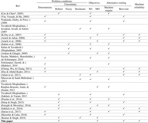
2. Literature review
Table 1. some researches in context of cellular manufacturing systems
Ref.
Problem conditions
Objectives Alternative routing
Machine reliability Deterministic
Uncertainty
Robust Fuzzy Stochastic SO MO Machine
require Best rout (
Cao & Chen*, 2005
)
( Yin, Yasuda, & Hu, 2005
)
( Nsakanda, Diaby, & Price,
2006
)
( Tavakkoli-Moghaddam, Javadian, Javadi, & Safaei,
2007 )
( K Das et al., 2007
)
( Ameli & Arkat, 2008
)
( Ameli et al., 2008
)
( Safaei et al., 2008
)
( Safaei &
Tavakkoli-Moghaddam, 2009
)
( Arıkan & Güngör, 2009
)
( Paydar, Mahdavi, Sharafuddin,
& Solimanpur, 2010
)
( Solimanpur, Saeedi, &
Mahdavi, 2010
)
( Chung, Wu, & Chang, 2011
)
( Das & Abdul-Kader, 2011
)
( Arkat et al., 2011
)
( Ghezavati & Saidi-Mehrabad,
2011
)
( Tavakkoli-Moghaddam, Ranjbar-Bourani, Amin, &
Siadat, 2012 )
( Tavakkoli-Moghaddam,
Sakhaii, & Vatani, 2013
)
( Paydar et al., 2014
)
( Deep & Singh, 2015
)
(Farughi & Mostafayi, 2016)
( Sakhaii et al., 2016
)
(Imran et al., 2017)
(Hazarika & Laha, 2018)
(Kumar & Singh, 2019)
This paper
Based on the investigated studies, design and reconfiguration of CMS under uncertainty conditions are presented by many researchers. This topic is important because appropriate forecasting of effective parameters in designing of manufacturing system is difficult and always has lack of enough accuracy. Also, with regard to nature of manufacturing systems and probability of occurring machines deterioration, designing of robust system to deal with changes in related parameters is an essential issue in manufacturing. Which yet did not have been investigated comprehensively. Actually, with regard to literature review, this paper design a robust multi objective model for planning of manufacturing parts for the first time with consideration of machines reliability that in is described completely section 1.
3. Machines reliability analysis in cellular manufacturing systems
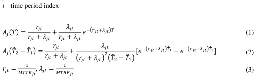
3.1. Machines availability
j machine index t time period index
(1) 𝐴𝑗(𝑇) =
𝑟𝑗𝑡 𝑟𝑗𝑡+ 𝜆𝑗𝑡+
𝜆𝑗𝑡 𝑟𝑗𝑡+ 𝜆𝑗𝑡𝑒
−(𝑟𝑗𝑡+𝜆𝑗𝑡)𝑇
(2) 𝐴𝑗(𝑇̂2− 𝑇̂1) = 𝑟𝑗𝑡
𝑟𝑗𝑡+ 𝜆𝑗𝑡+
𝜆𝑗𝑡
(𝑟𝑗𝑡+ 𝜆𝑗𝑡)2(𝑇̂2− 𝑇̂1)[𝑒
−(𝑟𝑗𝑡+𝜆𝑗𝑡)𝑇̂1− 𝑒−(𝑟𝑗𝑡+𝜆𝑗𝑡)𝑇̂2]
(3) 𝑟𝑗𝑡 =𝑀𝑇𝑇𝑅1
𝑗𝑡, 𝜆𝑗𝑡 =
1
𝑀𝑇𝐵𝐹𝑗𝑡
Which T is the time that machine j in time t is available. 𝐴𝑗(𝑇) Means the probability that machine j in time T is working. 𝐴𝑗(𝑇̂2− 𝑇̂1) Is availability interval of machine j in interval time
of 𝑇̂2↔ 𝑇̂1 in time period t. And 𝑟𝑗𝑡 , 𝜆𝑗𝑡 are repair rate and machine j deterioration rate within the interval time of t. The approach used in this article is such that machine effective capacity estimated by consideration of total capacity (total given time) within an interval and relate availability interval.
3.2 machines reliability model in a cellular manufacturing system
For explaining related problem in this article with regard to an example in research of (K Das et al., 2007) according table 2 information, manufacturing route for processing four part types on five machines are depicted. In this example, each part type may be manufactured by one of two possible process plans.
Table 2. manufacturing routes based on machines Part types Process plan Operations
1 2 3
1 1 M3, M2 M4, M5 M4
2 M2, M4 M3 M1, M4
2 1 M2 M4, M5 M3
2 M1, M3 M2 M5
3 1 M1, M4 M3, M2 M2
2 M4, M5 M2, M4 M1, M3
4 1 M1, M3 M2, M4 M5
2 M4, M5 M1 M4
According to table 2 each operation could be done on multiple machines which shows that each part can be processed in multiple process or in multiple machine routes. For example, part type 1, following process plan 1 has the options of performing operation 1 either on machine M3, or M2 and operation 2 either on M4 or M5. If we suppose one of the part type 1 process route in the form of rout1 {1, 2, 3} which that set {1, 2, 3} represents machines 1, 2, 3 in manufacturing route. The System reliability in this situation is as follows:
(4) 𝑅𝑠(𝑇) = 𝑅1(𝑇) × 𝑅2(𝑇) × 𝑅3(𝑇)
Here 𝑅𝑗(𝑇) is the reliability of machine j at time T, it means the probability that machine j is working within time t, or 𝑅𝑗(𝑇) = 𝑃𝑟(𝑇′≥ 𝑇). Where 𝑇′ is continuous random variable
defined as time to failure? Although equations 1 and 2 defined machines availability in terms of failure and repair rate for machines that are repairable. In this research we consider 𝑅𝑗(𝑇)
for selecting machines in cell configuration process. In next steps equation 4 convert to equation 5 to express system failure rate. Where is applicable to calculating reliability for repairable machines? We assume that machine failure time follow an exponential distribution. The reliability equality for machine j may be represented as:
𝑅𝑗(𝑇) = 𝑒−𝜆𝑗𝑡𝑇 Where 𝜆
𝑗𝑡 is the failure rate of machine j in time period t, when 𝑇 ≥ 0
represents time period number as 1, 2, etc. and T is the time duration in hours for the period number t). Then the system reliability equation 4 becomes: 𝑅𝑟𝑜𝑢𝑡1{1,2,3}(𝑇) = 𝑒− ∑𝑗∈1,2,3𝜆𝑗𝑡𝑇 .
Since T is planned time period of time and is the same for all considered machines. Hence the equation will be below:
(5) 1
ln{𝑅𝑟𝑜𝑢𝑡1{1,2,3}(𝑇)}×
1
𝑇 = ∑ 𝜆𝑗𝑡𝑇
𝑗∈1,2,3
= 𝐿𝐼𝑅𝑟𝑜𝑢𝑡1{1,2,3}𝑡
Where 𝐿𝐼𝑅𝑟𝑜𝑢𝑡1{1,2,3}𝑡 is the system failure rate for machines {M1,M2,M3} along the part
process route rout1{1, 2, 3} for a combined plan in {1, 2} at time period t. similarly 𝐿𝐼𝑅𝑖𝑝𝑡 represent all combination of parts process plans in time period t. minimizing 𝐿𝐼𝑅𝑖𝑝𝑡 improved
overall machines reliability in selected process plans for part types.
4. Problem definition
In this research a mixed integer programming bi-objective model represented for configuration of cellular manufacturing systems with alternative routes with consideration of machines reliability. The objectives of this model are included minimizing overall cost of system as first objective and minimizing the amount of machines failure as second objective. One of the notable points in this model is capable of dividing necessary operations for manufacturing one type part of various machines that can do it. Also, idle time of machines and cell is considered. It means that for assigning parts and machines to cells in order to we consider the costs related to movements and operations on parts, costs related to cells idle time with regard to reliability of machines are considered. This model chooses an appropriate machine in different process part routes and increase machine reliability and decrease system costs. Also, it is required new machines are purchased. More accurately we assume machines set 𝑗 = 1,2, … , 𝑚 for processing parts type 𝑖 = 1,2, … , 𝑛 or forecasting demand for periods 𝑡 = 1,2, …, is existed. 𝑇𝑡 Denotes time duration for period t. reliability parameters for machine j in period t are included: 𝑀𝑇𝐵𝐹𝑗𝑡 and 𝑀𝑇𝑇𝑅𝑗𝑡. Current machines reliability parameters at period 𝑡 = 1 are according to available data in each machine maintenance file. Based on manufacturer’s data and the maintenance history of machines, the reliability parameters for the next period can be estimated. Part type 𝑖 can be processed under any plans. A part-type process plan combination is denoted as (𝑖𝑝) and machines that can do operations 𝑂 related to (𝑖𝑝) represented by𝑗𝑖𝑝𝑜. Operation and
readjust costs for operation 𝑂 of (𝑖𝑝) on machine j are denoted as 𝐶𝑂𝑜𝑗(𝑖𝑝) and 𝐶𝑅𝑜𝑗(𝑖𝑝) and readjusting time is represented by 𝑇𝑂𝑜𝑗(𝑖𝑝) and 𝑇𝑅𝑜𝑗(𝑖𝑝) these costs and times within through planning horizon are known and constant. Based on available total capacity 𝑏𝑖𝑡 (in
hours) and availability 𝐴𝑗(𝑇𝑡), effective capacity of each machine (in hours) designated in each
costs. While system reliability maximized within planning horizon. Since in real world manufacturing parameters are influenced by environmental factors. We can’t designate exact value for them. In this model for considering this issue, we use uncertain parameters. Actually, different parameters value with regard to scenarios with specified probability are available. For solving model, we use robust optimization approach. Also presented model is a bi-objective model that we use LP-metric approach to solve it (Farughi & Mostafayi, 2016).
4.1. Mathematical model Indices
𝑐 Cells indices 𝑖 Parts indices 𝑝 Process plan indices
ip Alternative routing for part i in process plan p
𝑚 Machines indices
𝑗𝑖𝑝𝑜 Set of machines that can perform operation 𝑜 on 𝑖𝑝 route 𝑜 Operation indices
ℎ Time period indices 𝑠 Scenarios indices
Parameters
𝐴(𝑇ℎ)𝑚𝑠 Availability of machine j at time T in the period number h under scenario s
𝛼𝑚ℎ𝑠 Machine m holding cost at period h under scenario s
𝐶𝑂(𝑖𝑝)𝑜𝑚𝑠 Operation𝑜 process cost of 𝑖𝑝 on machine m under scenario s
𝐶𝑅(𝑖𝑝)𝑜𝑚𝑠 readjusting cost of process o of 𝑖𝑝 on machine m under scenario s
𝛿𝑚ℎ𝑠 cost of installation and uninstallation machine m at period h under scenario s
𝑇ℎ𝑠 Duration of period h under scenario s
𝜗𝑚ℎ𝑠 Cell idle time cost for machine 𝑚 at period h under scenario 𝑠 𝐶𝑃𝑚ℎ𝑠 cost of idle time of machine 𝑚 at period h under scenario𝑠
𝑇𝑂(𝑖𝑝)𝑚𝑜ℎ𝑠 Time needed to processing operation 𝑜 of 𝑖𝑝 by machine 𝑚 in period h under scenario
s
𝑇𝑅(𝑖𝑝)𝑚𝑜ℎ𝑠 Time needed to adjusting operation 𝑜 of 𝑖𝑝 by machine 𝑚 in period h under scenario
s
𝐶𝑀𝑚ℎ𝑠 cost of purchasing new capacity for machine m in period h under scenario s
𝜆𝑚ℎ𝑠 Failure coefficient for machine m in period h under scenario s
𝐴𝑣𝑚ℎ𝑠 Number of available machines type m in period h under scenario s
𝑈𝑀 Upper bound for cells capacity 𝐿𝑀 Lower bound for cells capacity
𝑟(𝑖𝑝)𝑜𝑚𝑠 equals 1 if operation 𝑜 needed machine m of 𝑖𝑝 under scenario s
𝐷𝑖ℎ𝑠 Demand of part 𝑖 in period h under scenario s
𝑏𝑚ℎ𝑠 Available time for machine m in period h under scenario s
Decision variables
𝑀𝑚𝑐𝑠 Binary variable will equal 1 if machine otherwise will be equal zero m assigned to cell c under scenario s
𝑁𝑚𝑐ℎ𝑠 Number of machine type m assigned to cell c in period h under scenario s
𝑍(𝑖𝑝)𝑜𝑚𝑐ℎ𝑠 Number of part type i manufactured under plan p by operation o on machine m in cell c at period h under scenario s
𝐾𝑚𝑐ℎ𝑠− Number of removed machines type m from cell c in period h under scenario s
𝑇𝑂𝑇𝑁𝑀𝑚𝑐ℎ𝑠 aggregated added capacities to machine m in cell c at period h under scenario s
𝑋(𝑖𝑝)𝑜𝑚𝑐ℎ𝑠 Binary variable will be equal 1 if part type m in cell c at period h under scenario s manufactured. Otherwise will equal to zero i under plan p by operation o on machine
𝑀𝑖𝑛𝑍1 = ∑ 𝑍𝑖
7
𝑖=1
𝑆. 𝑇
𝑍1 = ∑ ∑ ∑ ∑ 𝑁𝑚𝑐ℎ𝑠𝛼𝑚ℎ𝑠 𝑠=1 𝐻 ℎ=1 𝐶 𝑐=1 𝑀 𝑚=1 (6) 𝑍2 = ∑ ∑ ∑ ∑ ∑ ∑ ∑ 𝑍(𝑖𝑝)𝑜𝑚𝑐ℎ𝑠𝑇𝑅(𝑖𝑝)𝑚ℎ𝑠{𝐶𝑂(𝑖𝑝)𝑜𝑚𝑠 𝑠=1 𝐻 ℎ=1 𝐶 𝑐=1 𝑀 𝑚𝜖𝑚(𝑖𝑝𝑜) 𝑃(𝑖) 𝑝=1 𝑛 𝑖=1 𝑂(𝑖𝑝) 𝑜=1 + 𝐶𝑅(𝑖𝑝)𝑜𝑚} (7)
𝑍3= (1
2) ∑ ∑ ∑ ∑ ∑ ∑ | ∑ 𝑍(𝑖𝑝)(𝑜+1)𝑚𝑐ℎ𝑠− 𝑍(𝑖𝑝)𝑜𝑚𝑐ℎ𝑠
𝑀 𝑚=1 | 𝑃(𝑖) 𝑝=1 𝑠=1 𝑂 𝑜=1 𝑜<𝑂𝑃 𝑛 𝑖=1 𝐶 𝑐=1 𝐻 ℎ=1 (8)
𝑍4= ∑ ∑ ∑ ∑ 𝛿𝑚ℎ𝑠(𝐾𝑚𝑐ℎ𝑠+ + 𝐾
𝑚𝑐ℎ𝑠− ) 𝑆 𝑠=1 𝑀 𝑚=1 𝐶 𝑐=1 𝐻 ℎ=1 (9)
𝑍5≥ ∑ ∑ ∑ ((𝑇ℎ𝑠𝑁𝑚𝑐ℎ𝑠 𝑆 𝑠=1 𝑀 𝑚=1 𝐻 ℎ=1 − ∑ ∑ ∑ 𝑍(𝑖𝑝)𝑜𝑚𝑐ℎ𝑠𝑇𝑅(𝑖𝑝)𝑚ℎ𝑠 𝑛 𝑖=1 𝑂𝑃 𝑘=1 𝑝(𝑖) 𝑝=1 ) 𝜗𝑚ℎ𝑠) (10)
𝑍6= ∑ ∑ 𝐶𝑃𝑚ℎ𝑠(1 − 𝑀𝑈𝑇𝑚ℎ𝑠+ ∑ 𝑇𝑂𝑇𝑁𝑀𝑚𝑐ℎ𝑠
𝐶 𝑐=1 ) 𝑀 𝑚=1 𝐻 ℎ=1 (11) 𝑀𝑈𝑇𝑚ℎ= ∑ ∑ ∑ ∑ {𝑇𝑂(𝑖𝑝)𝑚ℎ𝑠+ 𝑇𝑅(𝑖𝑝)𝑚ℎ𝑠 𝐴𝑗(𝑇ℎ)𝑏𝑚ℎ𝑠 } 𝐶 𝑐=1 𝑂(𝑖𝑝) 𝑜=1 𝑃(𝑖) 𝑝=1 𝑛 𝑖=1
𝑍(𝑖𝑝)𝑜𝑚𝑐ℎ𝑠 ∀𝑚, ℎ, 𝑠 (12)
𝑍7= ∑ ∑ ∑ ∑ 𝐶𝑀𝑚ℎ𝑠𝑁𝑚𝑐ℎ𝑠
𝑆 𝑠=1 𝐻 ℎ=1 𝐶 𝑐=1 𝑀 𝑚=1 (13)
𝑀𝑖𝑛𝑍2 = ∑ ∑ ∑ ∑ ∑ ∑ ∑ 𝐿𝐼𝑅𝑖𝑝ℎ𝑠𝑋(𝑖𝑝)𝑜𝑚𝑐ℎ𝑠 𝑆 𝑠=1 𝐶 𝑐=1 𝑀 𝑚𝜖𝑚(𝑖𝑝𝑜) 𝑂(𝑖𝑝) 𝑜=1 𝑃(𝑖) 𝑝=1 𝑛 𝑖=1 𝐻 ℎ=1 (14) 𝑆. 𝑇 𝐿𝐼𝑅𝑖𝑝ℎ = ∑ 𝜆𝑚ℎ𝑠 𝑀 𝑚𝜖𝑚(𝑖𝑝𝑜)
∀𝑖, 𝑝, ℎ, 𝑠 (15)
∑ ∑ 𝑍(𝑖𝑝)𝑜𝑚𝑐ℎ𝑠 𝑄
𝑖=1 𝑀
𝑚=1
∑ 𝑁𝑚𝑐ℎ𝑠 𝐶
𝑐=1
≤ 𝐴𝑣𝑚ℎ𝑠 ∀𝑚, ℎ, 𝑠 (17)
∑ 𝑁𝑚𝑐ℎ𝑠
𝑀
𝑚=1
≤ 𝑈𝑀 ∀𝑐, ℎ, 𝑠 (18)
∑ 𝑁𝑚𝑐ℎ𝑠≥ 𝐿𝑀
𝑀
𝑚=1
∀𝑐, ℎ, 𝑠 (19)
∑ 𝑍(𝑖𝑝)𝑜𝑚𝑐ℎ𝑠 𝐶
𝑐=1
≤ 𝑀. 𝑟(𝑖𝑝)𝑜𝑚𝑠 ∀𝑚, 𝑐, ℎ, 𝑠 (20)
𝑁𝑚𝑐,ℎ−1,𝑠+ 𝐾𝑚𝑐ℎ𝑠+ − 𝐾
𝑚𝑐ℎ𝑠− = 𝑁𝑚𝑐ℎ𝑠 ∀𝑚, 𝑐, ℎ, 𝑠 (21)
∑ ∑ ∑ ∑ 𝑍(𝑖𝑝)𝑜𝑚𝑐ℎ𝑠
𝑃
𝑝=1
= 𝐷𝑖ℎ𝑠
𝑂
𝑜=1 𝑀
𝑚=1 𝐶
𝑐=1
∀𝑖, ℎ, 𝑠 (22)
𝑇𝑂𝑇𝑁𝑀𝑚𝑐ℎ𝑠= 𝑇𝑂𝑇𝑁𝑀𝑚𝑐(ℎ−1)𝑠+ 𝑁𝑚𝑐ℎ𝑠 ∀𝑚, 𝑐, ℎ, 𝑠 (23)
∑ ∑ ∑ 𝑍(𝑖𝑝)𝑜𝑚𝑐ℎ𝑠{𝑇𝑂(𝑖𝑝)𝑜𝑚𝑠+ 𝑇𝑅(𝑖𝑝)𝑜𝑚𝑠} 𝑂(𝑖𝑝)
𝑜=1 𝑃(𝑖)
𝑝=1 𝑛
𝑖=1
≤ 𝑏𝑚ℎ𝑠𝐴(𝑇ℎ)𝑗𝑠(𝑀𝑚𝑐𝑠+ 𝑇𝑂𝑇𝑁𝑀𝑚𝑐ℎ𝑠)
∀𝑚, 𝑐, ℎ, 𝑠 (24)
𝑋(𝑖𝑝)𝑜𝑚𝑐ℎ𝑠≤ 𝑍(𝑖𝑝)𝑜𝑚𝑐ℎ𝑠 ∀𝑖, 𝑝, 𝑜, 𝑚, 𝑐, ℎ, 𝑠 (25)
𝑍(𝑖𝑝)𝑜𝑚𝑐ℎ𝑠≤ 𝑀. 𝑋(𝑖𝑝)𝑜𝑚𝑐ℎ𝑠 ∀𝑖, 𝑝, 𝑜, 𝑚, 𝑐, ℎ, 𝑠 (26)
𝐾𝑚,𝑐,1,𝑠+ = 𝑁
𝑚,𝑐,1,𝑠 ∀𝑚, 𝑐, 𝑠 (27)
𝑁𝑚𝑐ℎ𝑠, 𝐾𝑚𝑐ℎ𝑠+ , 𝐾
𝑚𝑐ℎ𝑠− , 𝑍(𝑖𝑝)𝑜𝑚𝑐ℎ𝑠 ∀𝑖, 𝑝, 𝑜, 𝑚, 𝑐, ℎ, 𝑠 (28)
equal to total demands. Constraint (23) calculates the amount of added capacity to each machine. Constraint (24) ensures that number of operations assigned to each machine not be more than its maximum capacity. Constraints (25)-(28) define controlling constraints for decision variables of the model.
5. Robust optimization model framework
Robust optimization obtains a set of solutions that are robust against parameters (input data) fluctuations. The robust optimization approach represented by (Mulvey, Vanderbei, & Zenios, 1995). Robust optimization approach has much applications in operation research studies (Noorossana, Niaki, & Ershadi, 2014), (Babaee Tirkolaee, Alinaghian, Bakhshi Sasi, & Seyyed Esfahani, 2016), (Hejazi & Soleimanmeigouni, 2014). In this approach two types of robustness introduced. Solution robustness (near optimal solution in all scenarios) and model robustness (solution near to feasibility in all scenarios) the solution that obtain from the robust optimization model is called robust. If input data have changed so it remains near optimal, they called it solution robustness. A solution called robust if for little changes in input data it is almost feasible. This case is called model robustness. Robust optimization is included two specific constraints: 1) structural constraint, 2) controlling constraints. While Structural constraints are in the form of auxiliary constraints and formulated which influenced by uncertain data. In the following the framework of robust optimization explained briefly. At first 𝑥𝜖𝑅𝑛1 are designing variables vector and 𝑦𝜖𝑅𝑛2 is control variables vector. Robust
optimization model form is as follows:
(29) 𝑀𝑖𝑛𝑐𝑇𝑥 + 𝑑𝑇𝑦
(30) 𝐴𝑥 = 𝑏
(31) 𝐵𝑥 + 𝐶𝑦 = 𝑒
(32) 𝑥, 𝑦 ≥ 0
Constraint (30) is a structural constraint and its coefficient is constant and determine. Constraint (31) is controlling constraint which its coefficient is influenced by scenario and is non-deterministic. Constraint (32) ensures variables are non-negative. The formulation of robust optimization model is included a set of scenariosτ= {1,2, … S}. Under each scenario τϵ𝑆 the coefficients relate to controlling constraints are equal to {𝑑𝑠, 𝐵𝑠, 𝐶𝑠, 𝑒𝑠} with a constant
probability. Which 𝑃𝑠 represents the probability of occurring each scenario and ∑ 𝑃𝑠 𝑠 = 1. The
optimal solution of this model is robust if for each specific scenario 𝑆ϵ𝜏 is still near optimal. This case is called model robustness. There are conditions that maybe the solutions that obtain for above model aren’t both feasible and optimal for all scenarios 𝑆ϵ𝜏. At this point the relationship between solution robustness and model robustness are determined by multi criteria decision making concepts. For measuring this relationship robust optimization model is formulated. First of all control variable 𝑌𝑠 that for each scenario 𝑆ϵ𝜏 and error vector 𝛿𝑠 measured allowable infeasibility in control constraints under scenario s is introduced. Because of uncertain parameters the solution obtained by model maybe be infeasible for some scenarios therefore 𝛿𝑠 represents infeasibility of model under scenario s. if model be feasible 𝛿𝑠 will
equal zero. Otherwise 𝛿𝑠 will equal to a positive value according to constraint (35). Actually, the robustness measures unsatisfied demand model for manufacturing part. The robust optimization model based on mathematical programming (29) to (32) formulated as follows:
(33) 𝑀𝑖𝑛𝜎(𝑥, 𝑦1, … , 𝑦𝑠) + 𝜔𝜌(𝛿1, 𝛿2, … , 𝛿𝑠)
(34) 𝐴𝑋 = 𝑏
(35) 𝐵𝑠𝑥 + 𝐶𝑠𝑦𝑠+ 𝛿𝑠 = 𝑒𝑠
We must notice that because robust optimization model consider various scenarios, the first term in objective function is for selecting a unit for objective in previous objective function (33), ∆𝑠= 𝑐𝑇𝑥 + 𝑑𝑇𝑦 is a random variable with a random value equal to ∆𝑠= 𝑐𝑇𝑥 + 𝑑𝑠𝑇𝑦𝑠 with probability of 𝑃𝑠 under scenario𝑆ϵ𝜏. In random linear programming formulation, we used average value of 𝜎(0) = ∑ ∆𝑠 𝑠𝑃𝑠and actually the first term represents solution robustness.
The second term in objective function 𝜌(𝛿1, 𝛿2, … , 𝛿𝑠) is feasible penalty function which penalties violation of control constraints under some scenarios. Controlling constraint violation means infeasible solution obtained under some scenarios of problem. By using of weight 𝜔 relationship between solution robustness which measured by first term 𝜎(0) and model robustness which measured by penalty function 𝜌(0) we can model that under multi criteria decision making. Since our goal is minimizing 𝜎(0), it may be the solution be infeasible. If 𝜔increased enough, the term 𝜌(0) dominated and caused more cost. Studies about selecting appropriate 𝜌(0) and 𝜎(0) could find with checking (Mulvey et al., 1995; Yu & Li, 2000). The term σ(𝑥, 𝑦1, … , 𝑦𝑠) represented by (Mulvey et al., 1995) as follows:
(37) σ(0) = ∑ ∆𝑠𝑝𝑠+ 𝜆 ∑ 𝑝𝑠(∆𝑠− ∑ ∆𝑠′𝑝𝑠′
𝑆
𝑠′
)
2 𝑆
𝑠 𝑆
𝑠
To show the robustness of the solution, the variance of the equation (33) represents that decision has high risk. In other words, a little variation in parameters with uncertainty can cause huge changes in value of measurement function. 𝜆 Is assigned weight for solution variance. Viewed as a quadratic term exit in equation (34). (Yu & Li, 2000) used an absolute value instead of a quadratic term because of decreasing computational time which explained as follows:
(38) σ(0) = ∑ ∆𝑠𝑝𝑠+ 𝜆 ∑ 𝑝𝑠|∆𝑠− ∑ ∆𝑠′𝑝𝑠′
𝑆
𝑠′
|
𝑆
𝑠 𝑆
𝑠
5.1 The proposed model for robust optimization
In this study some parameters including cost of purchasing a machine, the variable cost of machine, cost of movement between cells in each category, cost of intra-cell movement, machine movement cost, holding cost of part and part demand parameter considered as uncertain and under scenarios. Based on the case study environment, production managers and some other experts cannot reach to an agreement for the exact amount of cost parameters. In fact, each expert presents cost parameters based on his calculations a experiences. Therefore, there are some different values for one parameter. In other word, there are some scenarios with certain probability for each value of parameters. Based on the nature of mentioned uncertainty of parameters, in this paper scenario based robust in used in order to handle the uncertainty of the parameters.
𝑇𝐶𝑠 = ∑ 𝑍𝑖𝑠
7
𝑖=1
(39)
𝑆. 𝑇
𝑍1𝑠 = ∑ ∑ ∑ 𝑁𝑚𝑐ℎ𝑠𝛼𝑚ℎ𝑠
𝐻 ℎ=1 𝐶 𝑐=1 𝑀 𝑚=1 (40)
𝑍2𝑠= ∑ ∑ ∑ ∑ ∑ ∑ 𝑍(𝑖𝑝)𝑜𝑚𝑐ℎ𝑠𝑡𝑜𝑖𝑚𝑠{𝐶𝑂(𝑖𝑝)𝑜𝑚𝑠
𝐻 ℎ=1 𝐶 𝑐=1 𝑀 𝑚𝜖𝑚(𝑖𝑝𝑜) 𝑃(𝑖) 𝑝=1 𝑛 𝑖=1 𝑂(𝑖𝑝) 𝑜=1 + 𝐶𝑅(𝑖𝑝)𝑜𝑚𝑠} (41)
𝑍3𝑠= (1
2) ∑ ∑ ∑ ∑ ∑ | ∑ 𝑍(𝑖𝑝)(𝑜+1)𝑚𝑐ℎ𝑠− 𝑍(𝑖𝑝)𝑜𝑚𝑐ℎ𝑠
𝑀 𝑚=1 | 𝑃(𝑖) 𝑝=1 𝑂 𝑜=1 𝑜<𝑂𝑃 𝑛 𝑖=1 𝐶 𝑐=1 𝐻 ℎ=1 (42)
𝑍4𝑠= ∑ ∑ ∑ 𝛿𝑚ℎ𝑠(𝐾𝑚𝑐ℎ𝑠+ + 𝐾
𝑚𝑐ℎ𝑠− ) 𝑀 𝑚=1 𝐶 𝑐=1 𝐻 ℎ=1 (43)
𝑍5𝑠≥ ∑ ((𝑇𝑚𝑠𝑁𝑚𝑐ℎ𝑠− ∑ ∑ ∑ 𝑍(𝑖𝑝)𝑜𝑚𝑐ℎ𝑠𝑡𝑜𝑖𝑚𝑠)𝜗𝑚ℎ𝑠) 𝑛 𝑖=1 𝑂𝑃 𝑘=1 𝑝(𝑖) 𝑝=1 𝑀 𝑚=1 (44)
𝑍6𝑠= ∑ ∑ 𝐶𝑃𝑚ℎ𝑠(1 − 𝑀𝑈𝑇𝑚ℎ𝑠+ ∑ 𝑇𝑂𝑇𝑁𝑀𝑚𝑐ℎ𝑠
𝐶 𝑐=1 ) 𝑀 𝑚=1 𝐻 ℎ=1 (45) 𝑀𝑈𝑇𝑚ℎ𝑠= ∑ ∑ ∑ ∑ {𝑇𝑂(𝑖𝑝)𝐴𝑚ℎ𝑠+ 𝑇𝑅(𝑖𝑝)𝑚ℎ𝑠 𝑗𝑠(𝑇ℎ)𝑏𝑚ℎ𝑠 } 𝐶 𝑐=1 𝑂(𝑖𝑝) 𝑜=1 𝑃(𝑖) 𝑝=1 𝑛 𝑖=1
𝑍(𝑖𝑝)𝑜𝑚𝑐ℎ𝑠 ∀𝑚, ℎ (46)
𝑍7𝑠= ∑ ∑ ∑ 𝐶𝑀𝑚ℎ𝑠𝑁𝑚𝑐ℎ𝑠
𝐻 ℎ=1 𝐶 𝑐=1 𝑀 𝑚=1 (47)
𝑅2𝑠 = ∑ ∑ ∑ ∑ ∑ ∑ 𝐿𝐼𝑅𝑖𝑝ℎ𝑠𝑋(𝑖𝑝)𝑜𝑚𝑐ℎ𝑠
𝐶 𝑐=1 𝑀 𝑚𝜖𝑚(𝑖𝑝𝑜) 𝑂(𝑖𝑝) 𝑜=1 𝑃(𝑖) 𝑝=1 𝑛 𝑖=1 𝐻 ℎ=1 (48) 𝐿𝐼𝑅𝑖𝑝ℎ𝑠= ∑ 𝜆𝑚ℎ𝑠 𝑀 𝑚𝜖𝑚(𝑖𝑝𝑜) (49)
Therefore, the robust optimization model for dynamic cell formation is depicted below, which in its only objective functions (50) and (51) an also constraint (52) has changed and other constraint are the same as pervious model.
𝑀𝑖𝑛𝑊1= ∑ 𝑃𝑠𝑇𝐶𝑠+ 𝜆1∑ 𝑃𝑠|𝑇𝐶𝑠− ∑ 𝑃𝑠′𝑇𝐶𝑠′ 𝑠′ | + 𝜔 ∑ ∑ ∑ 𝑃𝑠𝛿𝑖ℎ𝑠 ℎ 𝑖 𝑠 𝑠 𝑠 (50)
(∑ ∑ 𝑍(𝑖𝑝)𝑜𝑚𝑐ℎ𝑠
𝑀
𝑚=1 𝐶
𝑐=1
) + 𝛿𝑖ℎ𝑠= 𝐷𝑖ℎ𝑠 ∀𝑖, ℎ, 𝑠 (52)
Constraints 15-28
First and second term of first objective function are average and variance of total costs. Actually, these two terms measured the robustness of the solution. The third term of first objective measured model robustness with regard to control constraint infeasibility under scenario s.
The first objective function is nonlinear because has absolute value. And the problem will convert to a linear problem by introducing two new variables 𝑞1𝑠, 𝑝1𝑠. The constraint 𝑞1𝑠− 𝑝1𝑠 = 𝑇𝐶𝑠 − ∑ 𝑃𝑠′ 𝑠′𝑇𝐶𝑠′ added to main model. Also, the second objective function is
nonlinear because having absolute value term. And problem converting to a linear programming model with introducing two new variables 𝑞2𝑠, 𝑝2𝑠. Constraint 𝑞2𝑠−𝑝2𝑠 = 𝑅𝑠− ∑ 𝑃𝑠′ 𝑠′𝑅𝑠′ added to main model therefor the objective function of robust optimization model retyping as follows:
𝑀𝑖𝑛𝑊1= ∑ 𝑃𝑠𝑇𝐶𝑠+ 𝜆1∑ 𝑃𝑠(𝑞1𝑠+𝑝1𝑠) + 𝜔 ∑ ∑ ∑ 𝑃𝑠𝛿𝑖ℎ𝑠 ℎ
𝑖 𝑠 𝑠
𝑠
(53)
𝑀𝑖𝑛𝑊2= ∑ 𝑃𝑠𝑅𝑠+ 𝜆1∑ 𝑃𝑠(𝑞2𝑠+𝑝2𝑠) + 𝜔 ∑ ∑ ∑ 𝑃𝑠𝛿𝑖ℎ𝑠
ℎ 𝑖 𝑠 𝑠
𝑠
(54)
5.2 proposed process for solving model
The robust model presented in the previous section is a bi-objective programming problem. First of all, we must convert the problem to a single objective problem. For this purpose, with using of LP-metric we can do that (Lee, 1980). And replace the bi-objective problem with a single objective problem. Because two objectives are not in same scale at first, we normalize them by using equation (55) which 𝑊𝑖∗ is the optimal value for each objective. For the optimal model the two objectives are replaced by equation below and lead the problem to a single objective. In this study we assume that two objectives named by W1, W2 .Based on LP-metric method the robust optimization model for dynamic cell formation problem for each objective function solved separately. The objective function LP-metric model formulated as follows:
(55) 𝑀𝑖𝑛𝑊3= [𝑎 ×𝑤1− 𝑤1∗
𝑤1∗ ] + [(1 − 𝑎) ×
𝑤2− 𝑤2∗
𝑤2∗ ]
Where 0 ≤ 𝛼 ≤ 1 ,𝑤1∗ is optimal value of first objective and 𝑤2∗ is optima value of second objective. The coefficients are the weights for objective function in above equation. By using above equation, the bi-objective problem converts to a single objective problem and solved by CPLEX 12.1 solver in GAMS software.
6. Case study: A department of PISHGAMAN PICH PARS Co. with regard
to available data
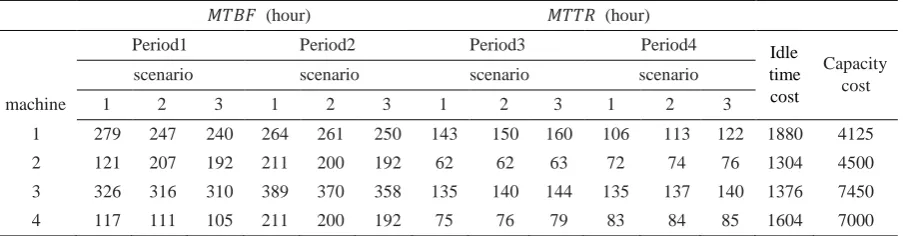
different types of bolts and washers like hexagon screws,Ajax bolt, hexagon nuts, sealed nuts and different types of washers and specific bolts according to global standards. One of the problems exists in this Co production planning which production managers deal with is cells configuration and assigning machines and parts without regarding to probability of machine breakdown. Actually, the current production planning is based on experience and sometimes caused to manufacturing system be stopped for a while. Which this short time cause to a lot of cost in production system. On the other, hand with regard to some dynamic parameters in planning such as forecasting amount of demand and then cost related to it and parameters related to machines and manufacturing system, planning only based on experience is very difficult. Consequently, experts and production manager of Co with regard to experience and consulting with experts and successful factories decide to plan with mathematical model. For this purpose, in this research a department above Co considered as a case study. Since whole data is not available for ruining model, because of reasons such as lack of appropriate recording of data to increasing confidence in accuracy and efficiency of data with agreeing of experts and experienced supervisors of manufacturing sector we used some data that exist in research of (Das & Abdul-Kader, 2011). This system manufactured 4 types’ parts in 3 manufacturing cell by 4 types of machine. And performed for 2 time period with regard to condition of presented model in this article. With considering problems such as price fluctuations in market, customers demand and etc. which manufacturing system always deal with them. The manger decides to optimize such parameters (costs, demand amount and etc.) under some scenarios. Aforementioned parameters under 3 scenarios with occurring probability of 0.2, 0.5 and 0.3 represented in table below:
Table 3. input data related to 𝑴𝑻𝑻𝑹,𝑴𝑻𝑩𝑭, machines idle time cost and purchasing machines capacity
𝑀𝑇𝐵𝐹 (hour) 𝑀𝑇𝑇𝑅 (hour)
Period1 Period2 Period3 Period4 Idle
time cost
Capacity cost
scenario scenario scenario scenario
machine 1 2 3 1 2 3 1 2 3 1 2 3
1 279 247 240 264 261 250 143 150 160 106 113 122 1880 4125
2 121 207 192 211 200 192 62 62 63 72 74 76 1304 4500
3 326 316 310 389 370 358 135 140 144 135 137 140 1376 7450
4 117 111 105 211 200 192 75 76 79 83 84 85 1604 7000
With regard to information in table above, if factory planning horizon considered monthly, based on previous data in work, averagely in month 25 days and daily 10 hours the factory is active, where obviously we can consider the length of planning horizon equals to (25 × 10) = 250 hours. Actually 𝑇1 = (0 − 250) and 𝑇2 = (250 − 500) . Therefore, with the help of equation (2) that explained in introduction section we can calculate machines availability. For example, availability of machine 2 in period 1 under scenario 1 is as follows:
(56)
𝐴2(𝑇1) = 𝐴2(𝑇12− 𝑇11) = 𝐴2(0 − 250)
= 1 62 (62 +1 212)1 +
1 212
(62 +1 212)1 2× (250 − 0)
× {1 − 𝑒−((
1
Where in it for calculating 𝜆𝑗𝑡 and 𝑟𝑗𝑡 we use equations 𝑟𝑗𝑡 =𝑀𝑇𝑇𝑅1
𝑗𝑡 and 𝜆𝑗𝑡 =
1
𝑀𝑇𝐵𝐹𝑗𝑡 for
example in above formula 𝑟21 =𝑀𝑇𝑇𝑅1
21=
1
62 and 𝜆21= 1
𝑀𝑇𝐵𝐹21=
1
212 . As represented
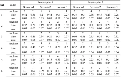
similarly for all machine we can calculate availability probability. Table below depicts operations on parts base on time, cost and machine type required, where actually is manufacturing route. For example, in manufacturing scheme 1 according to scenario 1, part 1 can be manufactured by routes that machines 2 and 3 in it. For other parts also there is a similar explanation.
Table 4. input data related to manufacturing cost and manufacturing time by machine in production plans
part index (process) plan 1 Process plan 2
Scenario1 Scenario2 Scenario3 Scenario1 Scenario2 Scenario3 1
machine 3 2 1 4 1 3 3 2 4 3 1 2 time 6.5 6.5 7.4 5 6.4 4.8 5.7 4.9 6.9 5.7 5 4.1
cost 1.09 1.06 0.82 0.63 0.87 1.02 0.76 0.73 1.08 0.78 0.98 0.95 2
machine 1 3 4 2 2 3 4 1 3 2 4 3 time 5.4 7.3 4 6.1 5.5 7.5 4.5 4.6 5.6 7.3 7.3 6.3
cost 0.66 0.97 0.76 0.7 0.63 0.65 1.13 1.11 0.93 0.65 1.08 0.82 3
machine 2 1 2 3 3 4 3 2 1 4 1 3 time 7.9 5.2 5.9 6.7 6.5 5.3 6.9 6.7 7.9 5 4.5 7.8
cost 0.63 1.16 0.74 0.9 1.14 0.9 0.64 0.76 0.78 0.84 0.74 1.16
4
machine 2 4 3 4 2 1 3 2 1 2 3 4 time 4.5 7.4 6.3 6.3 5.3 6.4 7.3 4.9 4.4 5.6 4.8 7.4
cost 1.10 1.11 0.98 0.93 0.78 0.66 0.98 0.85 0.88 0.79 0.94 0.91 5
machine 3 2 3 1 4 3 2 3 3 4 2 1 time 4.6 4.5 5.3 8 7.2 5.8 6.5 6.3 6.9 7 7.7 5.7
cost 1.08 0.79 1.11 1.01 0.83 0.8 0.89 1.16 0.73 1.06 1.13 0.64 6
machine 4 1 2 3 3 4 1 3 3 2 4 3 time 5.3 3 7.8 5.8 7.1 5.6 7.3 4.8 4.8 7.9 6.2 6.3
cost 0.73 0.89 0.61 0.76 1.12 0.98 0.82 0.84 0.68 1.08 1.13 1.03
Table 5. input data related cost information and re-adjusting time in production plans
part index Process plan 1 Process plan 2
Scenario1 Scenario2 Scenario3 Scenario1 Scenario2 Scenario3 1
machine 3 2 1 4 1 3 3 2 4 3 1 2 time 0.42 0.31 0.2 0.44 0.2 0.27 0.39 0.3 0.36 0.45 0.23 0.28 cost 0.05 0.06 0.05 0.05 0.07 0.06 0.05 0.05 0.07 0.05 0.05 0.06 2
machine 1 3 4 2 2 3 4 1 3 2 4 3 time 0.32 0.27 0.19 0.37 0.31 0.32 0.31 0.21 0.3 0.23 0.29 0.36 cost 0.05 0.05 0.07 0.06 0.05 0.07 0.05 0.06 0.05 0.06 0.05 0.07 3
machine 2 1 2 3 3 4 3 2 1 4 1 3 time 0.15 0.45 0.34 0.21 0.3 0.27 0.05 0.41 0.33 0.34 0.3 0.32 cost 0.07 0.06 0.07 0.05 0.07 0.07 0.06 0.05 0.05 0.07 0.07 0.06
4
machine 2 4 3 4 2 1 3 2 1 2 3 4 time 0.35 0.42 0.42 0.2 0.26 0.2 0.32 0.32 0.21 0.23 0.18 0.36 cost 0.06 0.07 0.07 0.06 0.06 0.05 0.06 0.06 0.06 0.05 0.07 0.06 5
machine 3 2 3 1 4 3 2 3 3 4 2 1 time 0.32 0.26 0.17 0.15 0.33 0.38 0.4 0.18 0.23 0.37 0.3 0.36 cost 0.07 0.05 0.07 0.07 0.06 0.06 0.05 0.05 0.06 0.05 0.06 0.05 6
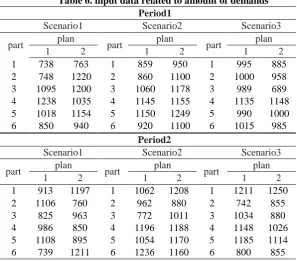
The amount of parts demand for manufacturing in planning horizon with regard to defines scenarios is according to table below. As observed the change in demand value sometime is significant. This change can be a result of importing external commodity or until seasonal changes and shutting down some construction project and etc. for example after shutting down of PADIDE Co construction projects, many of companies such as SAYBAN SAZEH TOOS which directly and semi-exclusively must manufacture required parts, and faced with serious problem to satisfying demands and orders.
Table 6. input data related to amount of demands Period1
Scenario1 Scenario2 Scenario3
part plan part plan part plan
1 2 1 2 1 2
1 738 763 1 859 950 1 995 885
2 748 1220 2 860 1100 2 1000 958
3 1095 1200 3 1060 1178 3 989 689
4 1238 1035 4 1145 1155 4 1135 1148
5 1018 1154 5 1150 1249 5 990 1000
6 850 940 6 920 1100 6 1015 985
Period2
Scenario1 Scenario2 Scenario3
part plan part plan part plan
1 2 1 2 1 2
1 913 1197 1 1062 1208 1 1211 1250
2 1106 760 2 962 880 2 742 855
3 825 963 3 772 1011 3 1034 880
4 986 850 4 1196 1188 4 1148 1026
5 1108 895 5 1054 1170 5 1185 1114
6 739 1211 6 1236 1160 6 800 855
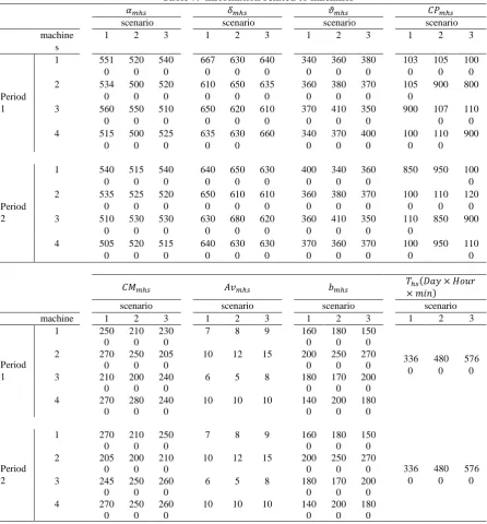
Table 7. information related to machines
𝛼𝑚ℎ𝑠 𝛿𝑚ℎ𝑠 𝜗𝑚ℎ𝑠 𝐶𝑃𝑚ℎ𝑠 scenario scenario scenario scenario machine
s
1 2 3 1 2 3 1 2 3 1 2 3
Period 1
1 551 0 520 0 540 0 667 0 630 0 640 0 340 0 360 0 380 0 103 0 105 0 100 0 2 534
0 500 0 520 0 610 0 650 0 635 0 360 0 380 0 370 0 105 0
900 800 3 560
0 550 0 510 0 650 0 620 0 610 0 370 0 410 0 350 0
900 107 0
110 0 4 515
0 500 0 525 0 635 0 630 0
660 340 0 370 0 400 0 100 0 110 0 900 Period 2
1 540 0 515 0 540 0 640 0 650 0 630 0 400 0 340 0 360 0
850 950 100 0 2 535
0 525 0 520 0 650 0 610 0 610 0 360 0 380 0 370 0 100 0 110 0 120 0 3 510
0 530 0 530 0 630 0 680 0 620 0 360 0 410 0 350 0 110 0
850 900 4 505
0 520 0 515 0 640 0 630 0 630 0 370 0 360 0 370 0 100 0
950 110 0
𝐶𝑀𝑚ℎ𝑠 𝐴𝑣𝑚ℎ𝑠 𝑏𝑚ℎ𝑠 𝑇× 𝑚𝑖𝑛)ℎ𝑠(𝐷𝑎𝑦 × 𝐻𝑜𝑢𝑟 scenario scenario scenario scenario machine 1 2 3 1 2 3 1 2 3 1 2 3
Period 1
1 250 0
210 0
230 0
7 8 9 160 0 180 0 150 0 336 0 480 0 576 0 2 270
0 250
0 205
0
10 12 15 200 0
250 0
270 0 3 210
0 200
0 240
0
6 5 8 180 0
170 0
200 0 4 270
0 280
0 240
0
10 10 10 140 0 200 0 180 0 Period 2
1 270 0
210 0
250 0
7 8 9 160 0 180 0 150 0 336 0 480 0 576 0 2 205
0 200
0 210
0
10 12 15 200 0
250 0
270 0 3 245
0 250
0 260
0
6 5 8 180 0
170 0
200 0 4 270
0 250
0 260
0
10 10 10 140 0
200 0
180 0
It is noteworthy that the probability of boom scenario is 0.45 medium scenario is 0.35 and low scenario: 0.2
Because of important of two objective function: total costs objective and summation of failure rate of machines, simultaneously three model for sensitivity analysis is represented:
Model W1: is including total system cost
Model W2: is including summation of failure rates in different periods and under different
scenarios and related constraints
Model W3: LP-metric Model is a combined from models W1 and W2 with related constraints.
These values obtained through interviewing with factory senior executives and with scrutiny past data (about amount of significance between manufacturing costs and production planning machine deterioration) which recorded periodically.
Table 8. Different weights for parameter 𝒂 0.43 1 0.29 5 0.36 4 0.34 4 0.29 6 0.16 6 0.42 9 0.31 7 0.16 4 0.38 7 0.41 8 0.32 3 0.26 3 0.25 5 0.43 7 0.12 3 0.39 6 0.16 8
0.25 0.24 4 0.28 1 0.30 2 0.17 9 0.17 2 0.32 6 0.25 4 0.22 7 0.20 5 0.23 3 0.34 1 0.25 8 0.17 8 0.23 5 0.19 2 0.21 9 0.30 4 0.16 4 0.14 3 0.21 9 0.33 6 0.43 7 0.41 4 0.33 2 0.31 7 0.34 8 0.15 9
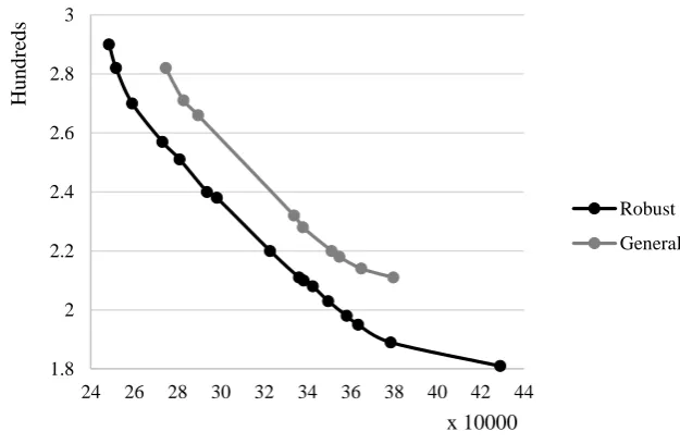
257 0.41 1 0.42 4 0.28 6 0.39 4 0.33 6 0.36 9 0.41 5 0.20 1 0.40 4 0.15 4 0.35 1 0.36 7 0.39 6 After solving model with GAMS software, by a computer with configuration 4GBRAM, CPU 3200 GHz – Core i5. The Pareto-front is according below:
Figure 1. Pareto fronts of the Robust Model and General Model
As observed the difference between solutions resulted from solving main problem and solution for solving robust model is absolutely tangible. Of course, we should mention that some solutions are dominated other solutions and don’t exist in any Pareto-front. Actually, above chart according to the definition of Pareto-front only represents non-dominated points. It is notable that in solving the problem we used𝜔 = 300, this value is calculated through checking robust problem represented in the next section.
6.1 analysis of problem robustness
In this section we investigate the relationship between model robustness and objective functions 𝑊1 and 𝑊2. Actually, in this scrutiny we specified model feasibility. If it isn’t feasible this amount of violation how impact on the objective function. As before mentioned, robustness means lack of sensitivity to changes in model input parameters. Also, we can cell a model is robust when for each scenario is almost feasible. According equations (53) and (54) model robustness is calculated by the third part of these equations. Actually variable 𝛿𝑖ℎ𝑠 is an error
vector which represents amount of infeasibility of model. Since this variable is always non-negative and sufficient ω is also positive, always the third part of the equations (53) and (54) is non-negative. Therefore, if for one specified value of ω (without changing other parameters)
1.8 2 2.2 2.4 2.6 2.8 3
24 26 28 30 32 34 36 38 40 42 44
there is no change in objective functions, we can say the error vector of model has a value of zero (δihs = 0) and model is feasible for all scenarios. For a specific value of α which is selected based on proposed weights as the final solution for implementing in a factory. We solve the problem for different value of ω and changes in the objective function value is checked. This action continues until the difference between objective function values become zero. (The model becomes feasible for all scenarios) the table below showed solution resulted from solving problem for each objective function and for different value of ω .
Table 9. robustness checking according to objective function 𝑾𝟏and 𝑾𝟐
𝑊2
𝑊1
ω 𝑊
3
𝑊2
𝑊1
𝑊3
𝑊2
𝑊1
17.978 152
653845 0
0 13410 100
18.109 162
710902 8.362
341 61055
200
18.908 171
823975 9.084
358 71122
300
19.659 181
865701 10.935
399 84133
400
20.711 181
912587 11.202
412 87049
500
21.108 181
987278 11.489
446 87097
600
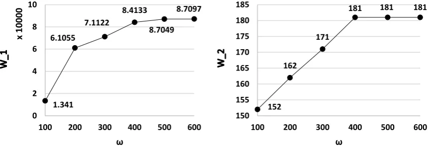
We observed that for the first objective function, for the value of ω= 600 the third part of the equation (53) is zero and model is feasible. Also, for second objective function the third part of the equation (54) in ω= 500 equals zero and model is feasible for all scenarios. This case can be seen in the figure 2.
Model Robustness according to 𝑊2objective function
Model Robustness according to 𝑊1 objective function
Figure 2. Model robustness for objective functions
In the following, for the purpose, analyzing problem the value of ω=300 considered and according to this value output result represented in table below. In this Table, we can see unsatisfied demands. As determined the value of error vector for part 1 under “high scenario’’ for the period 1 is a positive value. For this art demand is equal to 738 which optimal value of that is 579 units and the amount of unsatisfied demand is 159 units. For part 3 under ‘’high’’ scenario also observed in period 1 where the amount of demand is equal to 1059 units, the optimal manufactured is 951 and amount of unsatisfied demand is 108 units. In period 3 under “high” scenario some of parts has unsatisfied demands. This case showed that in value of ω = 300 some scenarios are infeasible model:
152 162
171
181 181 181
150 155 160 165 170 175 180 185
100 200 300 400 500 600
ω
1.341 6.1055
7.1122
8.4133
8.7049 8.7097
0 2 4 6 8 10
100 200 300 400 500 600
x
10000
Table 10. Unsatisfied demands under different scenarios 𝑃6 𝑃5 𝑃4 𝑃3 𝑃2 𝑃1 Scenarios 𝛿𝑝ℎ𝑠 0 0 0 108 0 159 boom
ℎ1 medium 0 0 0 0 0 0
0 0 0 0 0 0 low 351 0 298 0 102 0 boom
ℎ2 medium 0 0 0 0 0 0
0 0 0 0 0 0 low
Total costs of system under different scenarios are as follows:
Table 11. System costs under scenarios
Total failure rates Total costs Cost of purchasing new capacity Machines idle time costs Cell idle time cost Purchasing and removing cost of machine Parts movement costs between cells Performing operations cost Machines holding cost Scenario 227 390644 47143 72470 32896 61000 34051 59168 83916 Boom 202 319766 35697 49201 28642 47500 28413 68145 62168 Middle 194 221593 22593 28613 18726 31000 21176 49328 50157 Fair
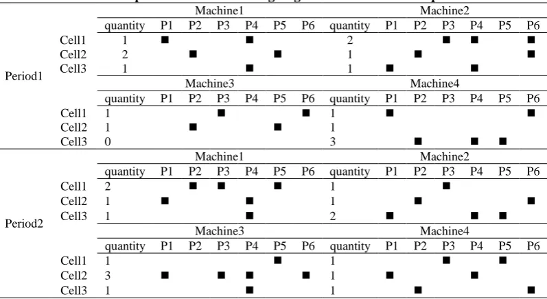
According to table above, we can observe system total cost from the scenario “high” to the scenario “low” is increased. The reason for this event is increasing trend of demand parameters and system cost. Of course, because of unsatisfied demand under scenario “high” for some parts, the performing operation cost doesn’t have increasing trend. The main structure of cell formation and also assigning machines to cells and also assigning parts to machines depicted in the table below:
Table 12. Output data related to assigning machines to cells and parts to machines
Period1
Machine1 Machine2
quantity P1 P2 P3 P4 P5 P6 quantity P1 P2 P3 P4 P5 P6
Cell1 1 2
Cell2 2 1
Cell3 1 1
Machine3 Machine4
quantity P1 P2 P3 P4 P5 P6 quantity P1 P2 P3 P4 P5 P6
Cell1 1 1
Cell2 1 1
Cell3 0 3
Period2
Machine1 Machine2
quantity P1 P2 P3 P4 P5 P6 quantity P1 P2 P3 P4 P5 P6
Cell1 2 1
Cell2 1 1
Cell3 1 2
Machine3 Machine4
quantity P1 P2 P3 P4 P5 P6 quantity P1 P2 P3 P4 P5 P6
Cell1 1 1
Cell2 3 1
Cell3 1 1
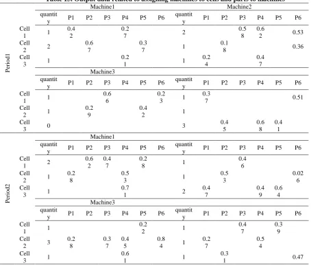
with regard to table (3) data according to scenario 1 used machines 2, 3 and based on scenario 2 used machines 1and 4 and finally based on scenario 3 used machines 1, 3 and for manufacturing using plan 1, also for using manufacturing plan2 could use the machine 2, 3 based on scenario 1, based on scenario 2 machines 3, 4 and finally based on scenario 3 machines 1, 2. However, according to the result, part 1 is manufactured based on scenario 2 of plan1 in cell 1, for this reason machine 1, 4 is in this cell. For other parts and machines, we can analyze similarly. The table below represents the duration of manufacturing operation for each part with regard to problem data and probability of each scenario.
Table 13. Output data related to assigning machines to cells and parts to machines
P
erio
d
1
Machine1 Machine2
quantit
y P1 P2 P3 P4 P5 P6
quantit
y P1 P2 P3 P4 P5 P6 Cell
1 1
0.4 2
0.2
7 2
0.5 8
0.6
2 0.53 Cell
2 2
0.6 7
0.3
7 1
0.1
8 0.36
Cell 3 1
0.2
1 1
0.2 4 0.4 7 Machine3 quantit
y P1 P2 P3 P4 P5 P6
quantit
y P1 P2 P3 P4 P5 P6 Cell
1 1
0.6 6
0.2 3 1
0.3
7 0.51
Cell 2 1
0.2 9
0.4
2 1
Cell
3 0 3
0.4 5 0.6 8 0.4 1 P erio d 2 Machine1 quantit
y P1 P2 P3 P4 P5 P6
quantit
y P1 P2 P3 P4 P5 P6 Cell
1 2
0.6 2
0.4 7
0.2
8 1
0.4 6 Cell
2 1
0.2 8
0.5
3 1
0.5 3
0.02 6 Cell
3 1
0.7
1 2
0.4 7 0.4 9 0.6 4 Machine3 quantit
y P1 P2 P3 P4 P5 P6
quantit
y P1 P2 P3 P4 P5 P6 Cell
1 1
0.2
2 1
0.4 7
0.3 9 Cell
2 3
0.2 8 0.3 7 0.4 5 0.8 4 1
0.2 7
0.5 4 Cell
3 1
0.6
1 1
0.3
1 0.47
6.2 Effective implications of the results and managerial insights In this section, the managerial implications are investigated as follows.
The computational results from the case study shows that the use of our proposed robust optimization approach led to minimize total cost and minimize the failure rate. Moreover, the solutions reduced the number of machines which are used in the system.
This study presented a scenario based robust approach to hedge against the uncertainty for the costs and so it enables a decision maker to obtain robust cell configuration decisions. The robust solution showed in better values for the first and the second objective functions.
7. Conclusion
Cellular manufacturing system (CMS) reconfiguration is a well-known method for improving productivity and competitiveness among manufactures. CMS tries to improve the whole system output and shorten the lead time by grouping specific products in small batches to be produced in a low cost and high-quality manufacturing cell. Despite all advantages of CMS, the shortcomings of such systems cannot be ignored. One of the most important disadvantages is the pause in the manufacturing process resulted from machine breakdowns. This issue is one of the most important concerns of planning managers. In this research, a bi-objective mixed integer mathematical model is presented for the reconfiguration of cellular manufacturing systems with alternative routes based on machines reliability. The objectives of this model include the minimization of the overall cost and minimization of the machine fails. Usually due to changes in the recorded data, to determine the exact amount for parameter used is difficult. Thus, to achieve better result and stay close to real world condition, the parameters are considered with uncertainty. To deal with such uncertainties and achieve promising results, the Mulvey robust programming is employed. To the best of the authors’ knowledge, in this research the CMS configuration is performed for the first time considering simultaneously both of the objective functions, namely the minimization of the overall cost and the minimization of machine failure under uncertainty condition in parameters. One significant advantage of the presented model is the sharing of operations required for manufacturing a part of machines in different cells that are capable to do those operations and have idle time. It means for assigning parts to machine and cells in addition to considering costs related to movement and operations on parts, cost related to cells idle time with regard to calculating machine reliability are considered. Due to the existence of two conflicting objective function in presenting a model, to have a better choice in selecting the final solution, solutions are represented as a Pareto - front. Also, to show the impact of using robust planning, set of non-dominated solution resulted from main problem and robust problem are compared with each other. Finally, decisions are compared to the opinion of the production planning experts at the PISHGAMAN PARS PICH Company as a case study. The Pareto-front and results are reported in detail. According to the results, using a robust programming method leads to improvement in objective function's values. This research can be used as a base for future research to extend the current model and to use Meta-heuristic algorithms to solve such complex models. Furthermore, using a fuzzy robust optimization approach might make this model to become more efficient and more useful to implement in manufacturing environments.
Acknowledgement
The authors would like to thank the staff of PISHGAMA PICH PARS Co for providing data and for their expertise, useful comments and the consultation.
References
Agarwal, A., and Sarkis, J., (1998). "A review and analysis of comparative performance studies on functional and cellular manufacturing layouts", Computers and industrial engineering, Vol. 34, No.1, pp. 77-89.
reliability consideration", The International Journal of Advanced Manufacturing Technology, Vol. 35(7-8), pp. 761-768.
Ameli, M. S. J., Arkat, J., and Barzinpour, F., (2008). "Modelling the effects of machine breakdowns in the generalized cell formation problem", The International Journal of Advanced Manufacturing Technology, Vol. 39(7-8), pp. 838-850.
Arıkan, F., and Güngör, Z., (2009). "Modeling of a manufacturing cell design problem with fuzzy multi-objective parametric programming", Mathematical and Computer Modelling, Vol. 50, No. 3, pp. 407-420.
Arkat, J., Naseri, F., and Ahmadizar, F., (2011). "A stochastic model for the generalised cell formation problem considering machine reliability", International Journal of Computer Integrated Manufacturing, Vol. 24, No. 12, pp. 1095-1102.
Askin, R. G., and Estrada, S., (1999). "Investigation of cellular manufacturing practices", Handbook of cellular manufacturing systems, pp. 25-34.
Babaee Tirkolaee, E., Alinaghian, M., Bakhshi Sasi, M., and Seyyed Esfahani, M., (2016). "Solving a robust capacitated arc routing problem using a hybrid simulated annealing algorithm: a waste collection application", Journal of Industrial Engineering and Management Studies, Vol. 3, No. 1, pp. 61-76. Bedworth, D. D., Henderson, M. R., and Wolfe, P. M., (1991). Computer-integrated design and manufacturing: McGraw-Hill, Inc.
Ben-Tal, A., and Nemirovski, A., (1998). "Robust convex optimization", Mathematics of operations research, Vol. 23, No. 4, pp. 769-805.
Ben-Tal, A., and Nemirovski, A., (1999). "Robust solutions of uncertain linear programs", Operations research letters, Vol. 25, No. 1, pp. 1-13.
Ben-Tal, A., and Nemirovski, A., (2000). "Robust solutions of linear programming problems contaminated with uncertain data", Mathematical programming, Vol. 88, No. 3, pp. 411-424.
Cao, D., and Chen, M., (2005). "A robust cell formation approach for varying product demands", International journal of production research, Vol. 43, No. 8, pp. 1587-1605.
Chung, S.-H., Wu, T.-H., and Chang, C.-C., (2011). "An efficient tabu search algorithm to the cell formation problem with alternative routings and machine reliability considerations", Computers and industrial engineering, Vol. 60, No. 1, pp. 7-15.
Das, K., and Abdul-Kader, W., (2011). "Consideration of dynamic changes in machine reliability and part demand: a cellular manufacturing systems design model", International journal of production research, Vol.49, No. 7, pp. 2123-2142.
Das, K., Lashkari, R., and Sengupta, S., (2007). "Machine reliability and preventive maintenance planning for cellular manufacturing systems", European Journal of Operational Research, Vol. 183, No. 1, pp. 162-180.
Deep, K., and Singh, P. K., (2015). "Design of robust cellular manufacturing system for dynamic part population considering multiple processing routes using genetic algorithm", Journal of Manufacturing Systems, Vol. 35, pp. 155-163.
El Ghaoui, L., and Lebret, H., (1997). "Robust solutions to least-squares problems with uncertain data", SIAM Journal on matrix analysis and applications, Vol.18, No. 4, pp. 1035-1064.
Erenay, B., Suer, G. A., Huang, J., and Maddisetty, S., (2015). "Comparison of layered cellular manufacturing system design approaches", Computers and industrial engineering, Vol. 85, pp. 346-358.
Ghezavati, V., and Saidi-Mehrabad, M., (2011). "An efficient hybrid self-learning method for stochastic cellular manufacturing problem: A queuing-based analysis", Expert Systems with Applications, Vol. 38, No. 3, pp. 1326-1335.
Han, B. T., Zhang, C. B., Sun, C. S., and Xu, C. J., (2006). "Reliability analysis of flexible manufacturing cells based on triangular fuzzy number", Communications in Statistics-Theory and Methods, Vol. 35, No. 10, pp. 1897-1907.
Hazarika, M., and Laha, D., (2018). "Genetic algorithm approach for machine cell formation with alternative routings", Materials Today: Proceedings, Vol. 5, No. 1, pp. 1766-1775.
Hejazi, T., Soleimanmeigouni, I., (2014). "A novel approach in robust group decision making for supply strategic planning", Journal of Industrial Engineering and Management Studies, Vol. 1, No. 1, pp. 20-30.
Imran, M., Kang, C., Lee, Y. H., Jahanzaib, M., and Aziz, H., (2017). "Cell formation in a cellular manufacturing system using simulation integrated hybrid genetic algorithm", Computers and industrial engineering, Vol. 105, pp. 123-135.
Kia, R., Baboli, A., Javadian, N., Tavakkoli-Moghaddam, R., Kazemi, M., and Khorrami, J., (2012). "Solving a group layout design model of a dynamic cellular manufacturing system with alternative process routings, lot splitting and flexible reconfiguration by simulated annealing", Computers and operations research, Vol. 39, No. 11, pp. 2642-2658.
Kia, R., Khaksar-Haghani, F., Javadian, N., and Tavakkoli-Moghaddam, R., (2014). "Solving a multi-floor layout design model of a dynamic cellular manufacturing system by an efficient genetic algorithm", Journal of Manufacturing Systems, Vol. 33, No. 1, pp. 218-232.
Kumar, R., and Singh, S. P., (2019). "Modified SA Algorithm for Bi-objective Robust Stochastic Cellular Facility Layout in Cellular Manufacturing Systems", Advanced Computing and Communication Technologies (pp. 19-33): Springer.
Lee, D.-T., (1980). "Two-dimensional Voronoi diagrams in the Lp-metric", J. ACM, Vol. 27, No. 4, pp. 604-618.
Mahdavi, I., Aalaei, A., Paydar, M. M., and Solimanpur, M., (2010). "Designing a mathematical model for dynamic cellular manufacturing systems considering production planning and worker assignment", Computers and Mathematics with Applications, Vol.60, No. 4, pp. 1014-1025.
Mulvey, J. M., Vanderbei, R. J., and Zenios, S. A., (1995). "Robust optimization of large-scale systems", Operations Research, Vol. 43, No.2, pp. 264-281.
Nodem, F. D., Kenné, J., and Gharbi, A., (2011). "Simultaneous control of production, repair/replacement and preventive maintenance of deteriorating manufacturing systems", International Journal of Production Economics, Vol. 134, No. 1, pp. 271-282.
Noorossana, R., Niaki, S. T. A., and Ershadi, M. J., (2014). "Economic and economic‐statistical designs of phase II profile monitoring", Quality and Reliability Engineering International, Vol. 30, No. 5, pp. 645-655.
Nsakanda, A. L., Diaby, M., and Price, W. L., (2006). "Hybrid genetic approach for solving large-scale capacitated cell formation problems with multiple routings", European Journal of Operational Research, Vol. 171, No. (3), pp. 1051-1070.
Paydar, M. M., Mahdavi, I., Sharafuddin, I., and Solimanpur, M., (2010). "Applying simulated annealing for designing cellular manufacturing systems using MDmTSP", Computers and industrial engineering, Vol. 59, No. 4, pp. 929-936.