Learning Theory Analysis for Association Rules
and Sequential Event Prediction
Cynthia Rudin [email protected]
Sloan School of Management
Massachusetts Institute of Technology 77 Massachusetts Avenue
Cambridge, MA 02139, USA
Benjamin Letham [email protected]
Operations Research Center
Massachusetts Institute of Technology 77 Massachusetts Avenue
Cambridge, MA 02139, USA
David Madigan [email protected]
Department of Statistics Columbia University 1255 Amsterdam Avenue New York, NY 10027, USA
Editor:John Shawe-Taylor
Abstract
We present a theoretical analysis for prediction algorithms based on association rules. As part of this analysis, we introduce a problem for which rules are particularly natural, called “sequential event prediction.” In sequential event prediction, events in a sequence are revealed one by one, and the goal is to determine which event will next be revealed. The training set is a collection of past sequences of events. An example application is to predict which item will next be placed into a customer’s online shopping cart, given his/her past purchases. In the context of this problem, algorithms based on association rules have distinct advantages over classical statistical and machine learning methods: they look at correlations based on subsets of co-occurring past events (items a and b imply item c), they can be applied to the sequential event prediction problem in a natural way, they can potentially handle the “cold start” problem where the training set is small, and they yield interpretable predictions. In this work, we present two algorithms that incorporate association rules. These algorithms can be used both for sequential event prediction and for supervised classification, and they are simple enough that they can possibly be understood by users, customers, patients, managers, etc. We provide generalization guarantees on these algorithms based on algorithmic stability analysis from statistical learning theory. We include a discussion of the strict minimum support threshold often used in association rule mining, and introduce an “adjusted confidence” measure that provides a weaker minimum support condition that has advantages over the strict minimum support. The paper brings together ideas from statistical learning theory, association rule mining and Bayesian analysis.
1. Introduction
Consider the problem of predicting the next event within a current event sequence, given a “sequence database” of past event sequences to learn from. We might wish to do this, for instance, using data generated by a customer placing items into the virtual basket of an online grocery store such as NYC’s Fresh Direct, Peapod by Stop & Shop, or Roche Bros. The customer adds items one by one into the current basket, creating a sequence of events. The customer has identified him- or herself, so that all past orders are known. After each item selection, a confirmation screen contains a small list of recommendations for items that are not already in the basket. If the store can find patterns within the customer’s past purchases, it may be able to accurately recommend the next item that the customer will add to the basket. Another example is to predict each next symptom of a sick patient, given the patient’s past sequence of symptoms and treatments, and a database of the timelines of symptoms and treatments for other patients. We call the problem of predicting these sequentially revealed events based on past sequences of events “sequential event prediction.”
In these examples, a subset of past events (for instance, a set of ingredients for a particular recipe) can be useful in predicting the next event. In order to make predictions using subsets of past events, we employassociation rules(Agrawal et al., 1993). An association rule in this setting is an implicationa→b(such aslettuce and carrots→tomatoes), whereais a subset of items, andbis a single item. The association rule approach has the distinct advantage in being able to directly model underlying conditional probabilitiesP(b|a) eschewing the linearity assumptions underlying many classical supervised classification, regression, and ranking methods. Rules also yield predictive models that are interpretable, meaning that for the rulea→b, it is clear thatbwas recommended becauseais satisfied.
The association rules approach makes predictions from subsets of co-occurring past events. Using subsets may make the estimation problem much easier, because it helps avoid problems with the curse of dimensionality. For instanceP(tomatoes | lettuce and carrots) could be much easier to estimate thanP(tomatoes|lettuce, carrots,pears, potatoes,ketchup,eggs,bread, etc.). This is precisely why learning algorithms created from rules can be helpful for the “cold start” problem in recommender systems, where predictions need to be made when there are not enough data available to accurately compute the full probability of a new item being purchased.
a minimum support. These are separate mechanisms, in the sense that it is possible to generalize with a somewhat small sample size and a large minimum support threshold, and it is also possible to generalize with a large sample size and no support threshold. We thus derive two types of bounds: large sample bounds, which scale with the sample size, and small sample bounds, which scale with the minimum support of rules. Using both large and small sample bounds (that is, the minimum of the two bounds) gives a complete picture. The large sample bounds are of order
O
(p1/m)as in classical analysis of supervised learning, wheremdenotes the number of event sequences in the database, that is, the number of past baskets ordered by the online grocery store customer.
Most of our bounds are derived using a specific notion of algorithmic stability called “pointwise hypothesis stability.” The original notions of algorithmic stability were invented in the 1970’s and have been revitalized recently (Devroye and Wagner, 1979; Bousquet and Elisseeff, 2002), the main idea being that algorithms may be better able to generalize if they are insensitive to small changes in the training data such as the removal or change of one training example. The pointwise hypothesis stability specifically considers the average change in loss that will occur at one of the training ex-amples if that example is removed from the training set. Our generalization analysis uses conditions on the minimum support of rules in order to bound the pointwise hypothesis stability.
There are two algorithms considered in this work. At the core of each algorithm is a method for rank-ordering association rules where the list of possible rules is generated using the customer’s past purchase history and subsets of items within the current basket. These algorithms build off of the rule mining literature that has been developing since the early 1990’s (Agrawal et al., 1993) by using an application-specific rule mining method as a subroutine. Our algorithms are interpretable in two different ways: the predictive model coming out of the algorithm is interpretable, and the whole algorithm for producing the predictive model is interpretable. In other words, the algorithms are straightforward enough that they can be understood by users, customers, patients, managers, etc. Further, the rules within the predictive model can provide a simple reason to the customer why an item might be relevant, or identify that a key ingredient is missing from a particular recipe. The rules provide “IF,THEN,ELSE” conditions, and yield models of the same form as those from the expert systems literature from the early days of artificial intelligence (Jackson, 1998). Many authors have emphasized the importance of interpretability and explanation in predictive modeling (see, for example, the work of Madigan et al., 1997).
The first of the two algorithms considered in this work uses a fixed minimum support threshold to exclude rules whose itemsets occur rarely. Then the remaining rules are ranked according to the “confidence,” which for rulea→b is the empirical probability that bwill be in the basket given thatais in the basket. The right-hand sides of the highest ranked rules will be recommended by the algorithm. However, the use of a strict minimum support threshold is problematic for several well-known reasons, for instance it is known that important rules (“nuggets,” which are rare but strong rules) are often excluded by a minimum support threshold condition.
accuracy on the training set (confidence), the rule that appears more frequently (higher support) achieves a higher adjusted confidence and is thus preferred over the other rule.
All of the bounds are tied to the measure of quality (the loss function) used within the analy-sis. We would like to directly compare the performance of algorithms for various settings of the adjusted confidence’sKparameter (and for the minimum support thresholdθ). It is problematic to have the loss defined using the sameK value as the algorithm, in that case we would be using a different method of evaluation for each setting ofK, and we would not be able to directly compare performance across different settings ofK. To allow a direct comparison, we select one reference value of the adjusted confidence, called Kr (r for “reference”), and the loss depends onKr rather than onK. The bounds are written generally in terms ofKr. The special caseKr=0 is where the algorithm is evaluated with respect to the confidence measure. The small sample bounds for the adjusted confidence algorithm have two terms: one that generally decreases withK(as the support increases, there is better generalization) and the other that decreases asK gets closer toKr(better generalization as the algorithm is closer to the way it is being measured). These two terms are thus agreeing ifKr>K and competing ifKr<K. In practice, the choice ofK can be determined in several ways:Kcan be manually determined (for instance by the customer), it can be set using side information as considered by McCormick et al. (2012), or it can be set via cross-validation on an extra hold-out set.
The novel elements of the paper include: 1) generalization analysis that incorporates the use of association rules, for both classification and sequential event prediction, 2) the algorithm based on adjusted confidence, where the adjusted confidence is a Bayesian version of the confidence, 3) the definition of a new supervised learning problem, namely sequential event prediction. The work falls in the intersection of several fields that are rarely connected: association rule mining and associative classification, supervised machine learning and generalization bounds from statistical learning theory, and Bayesian analysis.
In terms of applications, the definition of “sequential event prediction” was inspired by, but not restricted to, online grocery stores. Examples are Fresh Direct, Amazon.com grocery, and netgro-cer.com. Many supermarket chains with local outlets also offer an online shop-and-delivery option, such as Peapod (paired with Stop & Shop and Giant). Other online retailers and recommendation engines may benefit from ranking algorithms that are transparent to the user like amazon.com’s “customers who purchased this also purchased that” recommender system. The same techniques used to solve the sequential event prediction problem could be used in medical applications to pre-dict, for instance, the winners at each round of a tournament (e.g, the winners of games in a football season), or the next move of a video game player in order to design a more interesting game. The work of McCormick et al. (2012) contains a Bayesian algorithm, based on the analysis introduced in this paper, for predicting conditions of medical patients in a clinical trial. The work of Letham et al. (2013b) uses empirical risk minimization to solve sequential event prediction problems dealing with email recipient recommendation, healthcare, and cooking.
2. Derivation of Algorithms
We assume an interface similar to that of Fresh Direct, where users add items one by one into the basket. After each selection, a confirmation screen contains a handful of recommendations for items that are not already in the customer’s basket. The customer’s past orders are known.
The set of items is
X
, for instanceX
={apples, bananas, pears, etc};X
is the set of pos-sible events. The customer has a past history of orders S which is a collection of m baskets, S={zi}i=1,...,m,zi⊆X
;S is the sequence database. The customer’s current basket is usually de-noted byB⊂X
;Bis the current sequence. An algorithm usesBandSto find rulesa→b, where ais in the basket andbis not in the basket. For instance, ifsalsaandguacamoleare in the basket Band also ifsalsa, guacamoleandtortilla chipswere often purchased together inS, then the rule (salsaandguacamole)→tortilla chipsmight be used to recommendtortilla chips.The support of a, written Sup(a) or #a, is the number of times in the past the customer has ordered itemseta,
Sup(a):=#a:=
m
∑
i=1
1[a⊆zi].
Ifa=∅, meaning acontains no items, then #a:=∑i1=m. The confidence of a rulea→b is
denoted “Conf” or “fS,0”:
Conf(a→b):=fS,0(a,b):=
#(a∪b)
#a ,
the fraction of timesb is purchased given thata is purchased. It is an estimate of the conditional probability of b given a. Ultimately an algorithm should order rules by conditional probability; however, the rules that possess the highest confidence values often have a left-hand side with small support, and their confidence values do not yield good estimates for the true conditional probabili-ties. Note thata∪bis the union of the setawith itemb(the intersection is empty). In this work we introduce the “adjusted” confidence as a remedy for this problem: Theadjusted confidencefor rule a→bis:
fS,K(a,b) :=
#(a∪b)
#a+K . The adjusted confidence forK=0 is equivalent to the confidence.
The adjusted confidence is a particular Bayesian estimate of the confidence. Specifically, as-suming a beta prior distribution for the confidence, the posterior mean is given by:
ˆ
p=L+#(a∪b)
L+K+#a ,
where L andK denote the parameters of the beta prior distribution. The beta distribution is the “conjugate” prior distribution for a binomial likelihood. For the adjusted confidence we choose L=0. This choice yields the benefits of the lower bounds derived in the remainder of this section, and the stability properties described later. The prior for the adjusted confidence tends to bias rules towards thebottomof the ranked list. Any rule achieving a high adjusted confidence must overcome this bias.
• Collaborative filtering prior: haveL/(L+K) represent the probability of purchasing itemb given that itema was purchased, calculated over a subset of other customers. This biases estimates of the target user’s behavior towards the “average” user.
• Revenue management prior: choose LandK based on the item’s price, so more expensive items are more likely to be recommended.
• Time dependent prior: use only the customer’s most recent orders, and chooseL andK to summarize the user’s behavior before this point.
A rule cannot have a high adjusted confidence unless it has a large enough confidence and also a large enough support on the left-hand side. To see this, consider the case when we take fS,K(a,b) large, meaning for someη, we have fS,K(a,b)>η, implying:
Conf(a→b) = fS,0(a,b)>η #a+K
#a ≥η, Sup(a) =#a≥(#a+K)
#(a∪b)
#a+K
>(#a+K)η, implying Sup(a) =#a> ηK
1−η. (1)
And further, expression (1) implies:
Sup(a∪b) =#(a∪b)>η(#a+K)>ηK/(1−η).
Thus, rules attaining high values of adjusted confidence have a lower bound on confidence, and a lower bound on support of both the right and left-hand sides, which means a better estimate of the conditional probability. The bounds clearly do not provide any advantage whenK=0 and the confidence is used.
AsK increases, rules with low support are heavily penalized, so they tend not to be at the top of the list. On the other hand, such rules might be chosen when all other rules have low confidence. That is an advantage of having no firm minimum support cutoff: “nuggets” that have fairly low support may filter to the top. Figure 1 illustrates this by showing the support of rules ordered by adjusted confidence, for two values ofK, using a transactional data set “T25I10D10KN200” from the IBM Quest Market-Basket Synthetic Data Generator (Agrawal and Srikant, 1994) which mimics a retail data set.1 We use all rules with either one or no items on the left and one item on the right (as produced for instance by GenRules, presented in Algorithm 1). On each scatter plot, each of the rules is represented by a point. The rules are ordered on the x-axis by adjusted confidence, and the support of the rule is indicated on the y-axis. AsK increases, rules with the highest adjusted confidence are required to achieve a higher support, as can be seen from the gap in the lower left corner of the scatter plot for largerK.
We now formally state the recommendation algorithms. Both algorithms use a subroutine for mining association rules to generate a set of candidate rules. GenRules(Algorithm 1) is one of the simplest such rule mining algorithms, which in practice should be replaced by a rule mining algorithm that retrieves rules tailored to the application. There is a vast literature on such algorithms since the field of association rule mining evolved on their development,e.g.Apriori (Agrawal et al., 1993).GenRulesrequires a setAwhich is the set of allowed left-hand sides of rules.
K=0 K=10 K=50
Figure 1: Support vs. rank in adjusted confidence forK=0,10,50. Rules with the highest adjusted confidence are on the left.
Algorithm 1:Subroutine GenRules.
Input:(S,B,
X
), that is, past ordersS={zi}i=1,...,m,zi⊆X
, current basketB⊂X
, set of itemsX
Output: Set of all rules{aj→bj}jwherebj is a single item that is not in the basketB, and whereajis either a subset of items in the basketB, or else it is the empty set. Also the left-hand sideajmust be allowed (meaning it is inA). That is, output rules
{aj→bj}j such thatbj∈
X
\Bandaj⊆B⊂X
withaj∈A, oraj=∅.2.1 Max Confidence, Min Support Algorithm
The max confidence, min support algorithm, shown as Algorithm 2, is based on the idea of elimi-nating rules whose itemsets occur rarely, which is commonly done in the rule-mining literature. For this algorithm, the rules are ranked by confidence, and rules that do not achieve a predetermined fixed minimum support threshold are completely omitted. The algorithm recommends the right-hand sides from the top ranked rules. Specifically, ifcitems are to be recommended to the user, the algorithm picks the top rankedcdistinct items.
It is common that the minimum support threshold is imposed on the right and left side Sup(a∪
b)≥θ; however, as long as Sup(a) is large, we can get a reasonable estimate of P(b|a). In that sense, it is sufficient (and less restrictive) to impose the minimum support threshold on the left side: Sup(a)≥θ. Hereθis a number determined beforehand (for instance, the support of the left must be at least 5 items). In this work, we only have a required minimum support on the left side. As a technical note, we might worry about the minimum support threshold being so high that there are no rules that meet the threshold. This is actually not a major concern because of the minimum support being imposed only on the left-hand side: as long as m≥θ, all rules∅→b meet the minimum
support threshold.
The thresholded confidence is denoted by ¯fS,θ:
¯
Algorithm 2:Max Confidence, Min Support Algorithm.
Input: (θ,
X
,S,B,GenRules,c), that is, minimum threshold parameterθ, set of itemsX
, past ordersS={zi}i=1,...,m,zi⊆X
, current basketB⊂X
,GenRulesgenerates candidate rulesGenRules(S,B,X
) ={aj→bj}j, number of recommendationsc≥1Output: Recommendation List, which is a subset ofcitems in
X
1 ApplyGenRules(S,B,
X
)to get rules{aj→bj}jwhereaj is in the basketBandbj is not. 2 Compute score for each ruleaj→bjas ¯fS,θ(aj,bj) = fS,0(aj,bj) = #(a#ajj∪bj)when support#aj≥θ, and ¯fS,θ(aj,bj) =0 otherwise.
3 Reorder rules by decreasing score.
4 Find the topcrules with distinct right-hand sides, and let Recommendation List be the right-hand sides of these rules.
Algorithm 3:Adjusted Confidence Algorithm.
Input: (K,
X
,S,B,GenRules,c), that is, parameterK, set of itemsX
, past ordersS={zi}i=1,...,m,zi⊆
X
, current basketB⊂X
,GenRulesgenerates candidate rules GenRules(S,B,X
) ={aj→bj}j, number of recommendationsc≥1Output: Recommendation List, which is a subset ofcitems in
X
1 ApplyGenRules(S,B,
X
)to get rules{aj→bj}jwhereaj is in the basketBandbj is not.2 Compute adjusted confidence of each ruleaj→bj as fS,K(aj,bj) =##a(ajj∪bj+K).
3 Reorder rules by decreasing adjusted confidence.
4 Find the topcrules with distinct right-hand sides, and let Recommendation List be the
right-hand sides of these rules.
2.2 Adjusted Confidence Algorithm
The adjusted confidence algorithm is shown as Algorithm 3. A chosen value ofKis used to compute the adjusted confidence for each rule, and rules are then ranked according to adjusted confidence.
The definition of the adjusted confidence makes an implicit assumption that the order in which items were placed into previous baskets is irrelevant. It is easy to include a dependence on the order by defining a “directed” version of the adjusted confidence, and calculations can be adapted accordingly. The numerator of the adjusted confidence becomes the number of past orders wherea is placed in the basketbefore b.
fS(directed),K (a,b) = #{(a∪b):bfollowsa}
#a+K .
2.3 Rule Selection
corre-lations between items by creating “negation” items, such as¬b. As an example of using negation rules in the ice cream category, we impose that forvanilla to be on the right, bothchocolateand strawberryneed to be on the left, in either their usual form or negated. Of these, the rule that is used corresponds to the current basket. In that case,¬chocolate,¬strawberry→vanillacould have a high score in order to recommendvanillawhen chocolateandstrawberryare not in the basket, whereaschocolate,¬strawberry→vanillamight have a low score, conveying that sincechocolate is already in the basket thatvanillashould not be recommended. Alternatively, we could create a negation item¬ice creamindicating that the basket contains no ice cream presently, sosprinkles+
¬ice cream→vanillacould have a high score.
We can also use negation items on the right, where if there is a rulea→ ¬bthat receives a higher score (confidence or adjusted confidence) than any other rules recommendingb, we can choose not to recommendb. Rules can be designed to capture higher level correlations in specific regimes, for instance the allowed setAcan contain up to three items in one product category, but only two items in another. It is not practical in general to exhaustively enumerate and use all possible rules in a rule modeling algorithm due to problems with computational complexity. The key is to find a small but good set of rules, for instance the set of rules containing exhaustively all subsets of 1, 2, or 3 items on the left; or perhaps use the top rules that come out of the Apriori algorithm (Agrawal et al., 1993). In Section 7 we provide citations to surveys on association rule mining and associative classification that discuss this important issue of rule-construction and rule-engineering.
2.4 Modeling Assumption
The general modeling assumption that we make with the two algorithms above can be written as fol-lows, where current basketBis composed of itemsb1, . . .bt, andXiis the random variable governing whether itemiwill be placed into the basket next:
argmax i=1,...,m
i∈/B
P(Xi=1|Xb1=1,Xb2=1, . . . ,Xbt =1)
= argmax i=1,...,m
i∈/B
max a∈A a⊆{b1,...,bt}
P(Xi=1|Xa1 =1,Xa2 =1, . . .).
This expression states that the most likely item to be added next into the basket can be identified using a subset of items in the basket, denoteda. That subset is restricted to fall into a classAwhich is chosen based on the application at hand and the ease in which that subset can be searched. The setAdetermines the hypothesis space for learning, and it would be chosen differently as we move from the small sample regime to the large sample regime, so that the right side of this expression would eventually look just like the left side when the sample is large.
Our modeling assumption aligns with sequential event prediction, where only part of a sequence is available to make a prediction at timet. This is a case where standard linear modeling approaches do not naturally apply, since one would need to make a linear combination of terms, some of which are unrealized. We discuss this more in Appendix A.
3. Definition of Sequential Event Prediction
For simplicity in notation, at each time the algorithm recommends only one item,c=1. A basket z consists of an ordered (permuted) set of items, z∈2X×Π, where 2X is the set of all subsets of
X
, and Π is the set of permutations over at most|X|elements. We have a training set of m baskets S={zi}1...m that are the customer’s past orders. Denote z∼D
to mean that basket z is drawn randomly (iid) according to distributionD
over the space of possible items in baskets and permutations over those items, 2X×Π. The tth item added to the basket is writtenz·,t, where the dot is just a placeholder for the generic basketz. Thetth element of theith basket in the training set is writtenzi,t. We define the number of items in basketzbyTz, that is,Tz:=|z|. We introduce a generic scoring function fS:(a,b)7→Rwhereais a subset of items andbis a single item. Theinputato the score is{z·,1, . . . ,z·,t}or is a subset of{z·,1, . . . ,z·,t}. For now we letabe the full set
{z·,1, . . . ,z·,t}. The input bis an item that is not already in the basket, b∈
X
\{z·,1, . . . ,z·,t}. Thescoring function fScomes from an algorithm that takes data setSas input. We can consider fSto be parameterized, and the algorithm will learn the parameters of fSfromS.
If the score fS({z·,1, . . . ,z·,t},b)is larger than that of fS({z·,1, . . . ,z·,t},z·,t+1), it means that the algorithm recommended the wrong item. The loss function below counts the proportion of times this happens for each basket.
ℓ0−1(fS,z):= 1 Tz
Tz−1
∑
t=0
1 if fS({z·,1, . . . ,z·,t},z·,t+1)−maxb∈X\{z·,1,...,z·,t}fS({z·,1, . . . ,z·,t},b)≤0
0 otherwise.
(Note that ifzcontains all items in
X
, then the recommendation for the last item is deterministic, so we would not count it towards the loss.) The true error for sequential event prediction is an expectation of the loss with respect toD
, and is again a random variable since the training setSis random.TrueErr(fS):=Ez∼Dℓ0−1(fS,z).
The empirical risk is the average loss with respect toS:
EmpErr(fS):= 1
m m
∑
i=1
ℓ0−1(fS,zi).
The loss is bounded (by 1), the baskets are chosen independently, and the empirical risk is an average of iid random variables and the true risk is the expectation. Thus, the problem fits into the traditional scope of statistical learning, and the loss can be used within concentration arguments to obtain generalization bounds.
score. For instance, if we are using the adjusted confidence algorithm, fS({z·,1, . . . ,z·,t},b):= max
a∈A,a⊆{z·,1,...,z·,t}
fS,K(a,b).
The 0-1 loss is not smooth, so we will often use a smooth convex upper bound for the loss within the bounds. Specifically, for the way we have defined sequential event prediction, if any item has a higher score than the next item added, the algorithm incurs an error. (Even if that item is added later on, the algorithm incurs an error at this timestep.) To measure the size of that error, we can use the 0-1 loss, indicating whether or not our algorithm gave the highest score to the next item added. However, the 0-1 loss does not capture how close our algorithm was to correctly predicting the next item, though this information might be useful in determining how well the algorithm will generalize. We approximate the 0-1 loss using a modified loss that decays linearly near the discontinuity. This modified loss allows us to consider differences in adjusted confidence, not just whether one is larger than another:
|(adjusted conf. of highest-scoring-correct rule)
−(adjusted conf. of highest-scoring-incorrect rule)|.
However, as discussed in the introduction, if we adjust the loss function’s K value to match the adjusted confidenceKvalue, then we cannot fairly compare the algorithm’s performance using two different values ofK. An illustration of this point is that for largeK, all adjusted confidence values are≪1, and for smallK, the adjusted confidence can be≈1; differences in adjusted confidence for smallK cannot be directly compared to those for largeK. Since we want to directly compare performance asK is adjusted, we fix an evaluation measure that is separate from the choice ofK. Specifically, we use the difference in adjusted confidence values with respect to a referenceKr:
|({adjusted conf.}Krof highest-scoring-correct ruleK)
−({adjusted conf.}Krof highest-scoring-incorrect ruleK)|. (2) The reference Kr is a parameter of the loss function, whereasK is a parameter of an algorithm. We setKr=0 to measure loss using the difference in confidence, andK=0 for an algorithm that chooses rules according to the confidence. AsKgets farther fromKr, the algorithm is more distant from the way it is being evaluated, which leads to worse generalization. Note that forKr=K, the 0-1 loss is the same as the sign of (2).
A similar loss will be used in classification, where we incur an error if the adjusted confidence of the incorrect label is higher than that of the correct label.
4. Generalization
Our goal in this section is to provide a foundation for supervised learning with association rules, and also a foundation for sequential event prediction. We will consider several quantities that may be important in the learning process: m,K orθ, the size of the set of possible itemsets|A|, and the probability of the least probable itemsets and items.
corresponding to the higher of the two scores. Max-score association rule classifiers are a special type of “associative classifier” (Liu et al., 1998) and are also a type of “decision list” (Rivest, 1987). The result in 4.2 is a uniform bound based on the VC dimension of the set of max-score classifiers. This bound does not depend explicitly onK, which we hypothesize is an important quantity for the learning process.
In order to understand howKmight affect learning, we use algorithmic stability analysis. This approach originated in the 1970’s (Rogers and Wagner, 1978; Devroye and Wagner, 1979) and was revitalized by Bousquet and Elisseeff (2002). Stability bounds depend on how the space of functions is searched by the algorithm (rather than the size of the function space), so it often yields more insightful bounds. These bounds are still not often directly useful due to large multiplicative constants (in our case a factor of 6), but they capture more closely the scalability relationship of a particular algorithm with respect to important quantities in the learning process. The calculation required for an algorithmic stability bound is to show that the empirical error will not dramatically change by altering or removing one of the training examples and re-running the algorithm. There are many different ways to measure the stability of an algorithm; most of the bounds presented here use a specific type of algorithmic stability (pointwise hypothesis stability) so that the bounds scale correctly with the number of training examplesm.
Section 4.1 presents a basic stability bound for sequential event prediction. Section 4.2 presents a uniform VC bound for classification with max-score classifiers. Section 4.3 provides notation. Section 4.4 presents another basic stability bound for sequential event prediction, for a rule-based loss function. We then focus on stability bounds for the rule-based algorithms provided in Section 2. Specifically, Section 4.5 provides stability bounds for the large sample asymptotic regime (for both sequential event prediction and classification). Then we consider the new smallmregime in Section 4.6, starting with stability bounds that formally show that minimum support thresholds can lead to better generalization (for both sequential event prediction and classification). From there, we present small sample bounds for the adjusted confidence algorithm, for classification and (separately) for sequential event prediction.
We note that the space of possible baskets (up to a maximum size) is a combinatorially large, discrete space. Because the space is discrete, all probability estimates converge to the true proba-bilities, which means that an algorithm that is statistically consistent can be obtained by estimating p(b|B)directly for the current basketB. Ifmis large, prediction is easy. The difficult part is when we have only enough data to well estimate conditionals that are much smaller,P(b|a),a⊂B. That is the problem we are concerned with. Consistency does not imply anything about generalization bounds for the finite sample case.
4.1 General Stability Bound for Sequential Event Prediction
In this section we provide a basic stability-based bound for sequential event prediction, by analogy with Theorem 17 of Bousquet and Elisseeff (2002) (B&E).
We define a sequential event prediction algorithm producing fSto havestrong sequential event prediction stabilityβ(by analogy with B&E Definition 15) if the following holds:
∀S∈
D
m,∀i∈ {1, ...,m}where the∞-norm is over baskets. A definition we will use from B&E is as follows: an algorithm producing function fSwithuniform stabilityβ′obeys:
∀S,∀i∈ {1, ...,m},kℓ(fS,·)−ℓ(fS/i,·)k∞≤β′.
Let us define a modified loss function. Let symbol∆temporarily denote fS({z·,1, . . . ,z·,t},z·,t+1)− maxb∈X\{z·,1,...,z·,t}fS({z·,1, . . . ,z·,t},b)in the expression below. The loss is:
ℓγ(fS,z):= 1 Tz
Tz−1
∑
t=0
1 if∆≤0 1−1
γ∆ if 0≤∆≤γ 0 if∆≥γ.
The empirical error and leave-one-out error defined for this loss are:
EmpErrγ(fS,zi) := 1 m
m
∑
i=1
ℓγ(fS,zi),
LooErrγ(fS,zi) := 1 m
m
∑
i=1
ℓγ(fS/i,zi).
Lemma 1 A sequential event prediction algorithm producing fSwith strong sequential event pre-diction stabilityβhas uniform stability2β/γwith respect to the loss functionℓγ.
Proof
|ℓγ(fS,z)−ℓγ(fS/i,z)|
≤ 1
Tz Tz−1
∑
t=0 1
γ
fS({z·,1, . . . ,z·,t},z·,t+1)− max b∈X\{z·,1,...,z·,t}
fS({z·,1, . . . ,z·,t},b)
−
fS/i({z·,1, . . . ,z·,t},z·,t+1)− max b∈X\{z·,1,...,z·,t}
fS/i({z·,1, . . . ,z·,t},b)
≤ 1
γ
1 Tz
Tz−1
∑
t=0
[|fS({z·,1, . . . ,z·,t},z·,t+1)−fS/i({z·,1, . . . ,z·,t},z·,t+1)|+
max b∈X\{z·,1,...,z·,t}
fS({z·,1, . . . ,z·,t},b)− max b∈X\{z·,1,...,z·,t}
fS/i({z·,1, . . . ,z·,t},b)
≤1
γ2β.
The first inequality uses the Lipschitz property of the loss, as well as an upper bound from moving the absolute values inside the sum. The third inequality uses the strong stability with respect to fS.
Theorem 2 Let fSbe a sequential event prediction algorithm with sequential event stabilityβ. Then for allγ>0and any m≥1and anyδ∈(0,1)with probability at least1−δover the random draw of sample S,
TrueErr(fS)≤EmpErrγ(fS) +4β
γ +
8mβ
γ+1 r
ln(1/δ)
2m and with probability at least1−δover the random draw of sample S,
TrueErr(fS)≤LooErrγ(fS) +4β
γ +
8mβ
γ+1 r
ln(1/δ)
2m .
As with classification algorithms, the type of stability one would need to apply these bounds can be quite difficult to achieve, as it requires that the change in the model is small for any training set when any example is removed. This is particularly difficult to achieve when the sample size is somewhat small. For the association rule bounds, we know that uniform stability is not possible for many algorithms that perform well. However, there are some algorithms that do exhibit stronger stability, as we will discuss.
4.2 Classification with Association Rules: A Uniform Bound
In the classification problem, each basket receives a single label that is one of two possible labels
{+1,−1}. This contrasts with sequential event prediction where there is a sequence of labels, one for each item in the basket as it arrives. For classification, we represent basketx as a binary vector, where entry j is 1 if item j is in the basket. We sample baskets with labels, z= (x,y), where x∈2X is a set of items (or, equivalently, a binary feature vector) and y∈ {−1,1} is the corresponding label. Each labeled basketz is chosen randomly (iid) from a fixed (but unknown) probability distribution
D
over baskets and labels. Given a training setSofmlabeled baskets, we wish to construct a classifier that can assign the correct label to new, unlabeled baskets. We begin by defining a scoring functiong:A× {−1,1} →R that assigns a score g(a,y) to a rule a→y.The set of left-hand sides A can be any collection of itemsets so long as every x∈2X contains at least one a∈A. We define a valid scoring function as one where∀a∈A, g(a,1)6=g(a,−1)
and∀a1,a2∈A, maxy∈{−1,1}g(a1,y)6=maxy∈{−1,1}g(a2,y), that is, there are no ties. The validity requirement will be discussed in the following paragraph. Define G to be the class of all valid scoring functions. We now define a class of decision functions that use a valid scoring function g∈Gto provide a label to a basketx, fg: 2X → {−1,1}. The decision function assigns the label corresponding to the highest scoring rule whose left-hand side is contained inx. Specifically,
fg(x) = argmax y∈{−1,1}
max
a∈A,a⊆xg(a,y). (3) We call such a classifier a “max-score association rule classifier” (or “decision list”) because it uses the association rule with the maximum score to perform the classification. Let
F
maxscore be the class of all max-score association rule classifiers:F
maxscore:={fg:g∈G}. We will bound the VC dimension of classF
maxscore. By definition, the VC dimension is the size of the largest set of baskets to which arbitrary labels can be assigned using some fg∈F
maxscore; it is the size of the largest set that can be shattered.g(a,y) =0 for alla andy. In this case the VC dimension can be considered to be infinite, which motivates our definition of a valid scoring function. This problem actually happens with any clas-sification problem where function f(x) =0∀xis within the hypothesis space, thereby allowing all points to sit on the decision boundary. Our definition of validity is equivalent to one in which ties are allowed but are broken deterministically using a pre-determined ordering on the rules. In practice, ties are generally broken in a deterministic way by the computer, so the inclusion of the function
f =0 is not problematic.
The true error of the max-score association rule classifier is the expected misclassification error: TrueErrClass(fg):=E(x,y)∼D1
[fg(x)6=y]. (4) The empirical error is the average misclassification error over a training set ofmbaskets:
EmpErrClass(fg):= 1
m m
∑
i=1
1[fg(xi)6=yi].
The main result of this subsection is the following theorem, which indicates that the size of the allowed set of left-hand sides may influence generalization.
Theorem 3 (VC Dimension for Classification)
The VC dimension h of the set of max-score classifiers is equal to the size of the allowed set of left hand sides of rules:
VCdim(
F
maxscore):=h:=|A|.From this theorem, classical results such as those of Vapnik (1999, Equations 20 and 21) can be directly applied to obtain a generalization bound:
Corollary 4 (Uniform Generalization Bound for Classification)
With probability at least1−δthe following holds simultaneously for all fg∈
F
maxscore:TrueErrClass(fg)≤EmpErrClass(fg) +ε
2 1+
r
1+4EmpErrClass(fg)
ε
!
,
whereε=4
|A|ln2m|A|+1−lnδ
m .
Note 1 (on uniform bounds): The result of Theorem 3 holds generally, well beyond the simple adjusted confidence or max confidence, min support algorithms. Those two algorithms correspond to specific choices of the scoring function g: the adjusted confidence algorithm takes g(a,y) =
fS,K(a,y), and the max confidence, min support algorithm takesg(a,y) = f¯S,θ(a,y). We could use other strategies to chooseg, for example, choosing fg∈
F
to minimize an empirical risk (similar to what we do in Letham et al., 2013c).proof of Theorem 3 (in Section 5), it can be seen thath≤ |A|even when A contains general boolean association rules. Thus the bound in Corollary 4 extends to boolean operators.
Note 3 (dependence on|A|): We can use a standard argument involving Hoeffding’s inequality and the union bound over elements of
F
maxscoreto obtain that with probability at least 1−δ, the following holds for all fg∈F
maxscore:TrueErrClass(fg)≤EmpErrClass(fg) +
s
1 2m
ln(2|Fmaxscore|) +ln 1
δ
.
The value of|
F
maxscore|is at most 2|A|. This is because there are|A|ways to determine maxa∈A,a⊆xg(a,y), and there are 2 ways to determine the argmax overy. The bound then depends onp|A|(as classical VC bounds would also give, using Theorem 3), but not log|A|. Note that the bound is meaningful when|A|<mso that 2|A|<2m.
Note 4 (on reducing|A|): It is possible that many of the possible left-hand sides in|A|are realized with zero probability. (This depends on the unknown probability distribution that the examples are drawn from.) Because of this, if we are willing to redefineA to include only realizable left-hand sides,|A|can be replaced in the bound by|A|, where
A
={a∈A:Pz(a⊆x)>0}are the itemsets that have some probability of being chosen.4.3 Notation for Algorithmic Stability Bounds
We will now introduce the notation that will be used for the algorithmic stability bounds, first for classification and then for sequential event prediction.
4.3.1 NOTATION FORCLASSIFICATIONBOUNDS
Recall that we samplez= (x,y)wherex∈2X is a set of items andy∈ {−1,1}is the corresponding label. Eachzis sampled randomly (iid) according to a distribution
D
over the space 2X× {−1,1}. The adjusted confidence algorithm uses the training setSofmiid baskets to compute the adjusted confidences fS,K and find a rule that will be used to label the basket. We usez= (x,y)to refer to a general labeled basket, andzi= (xi,yi)to refer specifically to theith labeled basket in the training set. We define a highest-scoring-correctrule forx as a rule with the highest adjusted confidence that predicts the correct labely. The left-hand side of a highest-scoring-correct rule obeys:a+SxK∈ argmax
a⊆x,a∈A fS,K(a,y) =
argmax a⊆x,a∈A
#(a∪y)
#a+K ,
whereK≥0. If more than one rule is tied for the maximum adjusted confidence, one can now be chosen randomly. If the true labelyis not found in the training set, then the confidence of all rules withy on the right-hand side will be 0, and we take∅→yas the maximizing rule. We define a
highest-scoring incorrectrule forxas a rule with the highest adjusted confidence that predicts the incorrect label−y, so the left-hand side obeys:
a-SxK ∈ argmax
a⊆x,a∈A fS,K(a,−y) =
argmax a⊆x,a∈A
#(a∪ −y)
Again, if the label−y is not found in the training set, we take∅→ −y as the maximizing rule.
Otherwise, ties are broken randomly.
A misclassification error is made for labeled basket z when the highest-scoring-correct rule, a+SxK →y, has a lower adjusted confidence than the highest-scoring incorrect rulea-SxK → −y. As discussed earlier, we will measure this difference in adjusted confidence values with respect to a referenceKr in order to allow comparisons with different values ofK. We will takeKr≥0. This leads to the definition of the 0-1 loss for classification:
ℓclass
0−1,Kr(fS,K,z):=
1 if fS,Kr(a+SxK,y)−fS,Kr(a-SxK,−y)≤0 0 otherwise.
The term fS,Kr(a+SxK,y)−fS,Kr(a-SxK,−y) is the “margin” of example z (that is, the gap in score between the predictions for the two classes, see also Shen and Wang, 2007).
We will now define the true error which, whenK=Kr, is a specific case of TrueErrClass defined in (4). (The functiongis chosen using the data set, and it is fS,K.) The true error is an expectation of a loss function with respect to
D
, and is a random variable since the training setS is random, S∼D
m.TrueErrClass(fS,K,Kr):=Ez∼Dℓclass0−1,Kr(fS,K,z). We approximate the true error using a different lossℓclass
γ,Kr that is a continuous upper bound on the 0-1 lossℓclass
0−1,Kr. It is defined with respect toKrand another real-valued parameterγ>0 as follows:
ℓclassγ,Kr(fS,K,z):=cγ(fS,Kr(a+SxK,y)−fS,Kr(a-SxK,−y)), wherecγ:R→[0,1],
cγ(y) =
1 fory≤0 1−y/γ for 0≤y≤γ
0 fory≥γ.
Asγapproaches 0, losscγapproaches the standard 0-1 loss. Also,ℓclass0−1,Kr(fS,K,z)≤ℓclassγ,Kr(fS,K,z). We define TrueErrClassγusing this loss:
TrueErrClassγ(fS,K,Kr) =Ez∼Dℓclassγ,Kr(fS,K,z),
where TrueErrClass≤TrueErrClassγ. The generalization bounds for classification will bound TrueErrClass by considering the difference between TrueErrClassγ and its empirical counterpart that we will soon define. For training basketxi, the left-hand side of a highest-scoring-correct rule obeys:
a+SxiK∈ argmax
a⊆xi,a∈AfS,K(a,yi), and the left-hand side of a highest-scoring-incorrect rule obeys:
a-SxiK∈ argmax
a⊆xi,a∈AfS,K(a,−yi).
The empirical error is an average of the loss over the baskets:
EmpErrClassγ(fS,K,Kr):= 1 m
m
∑
i=1
For the max confidence, min support algorithm, we substituteθwhereKappears in the notation. For instance, for general labeled basketz= (x,y), we analogously define:
a+Sxθ ∈ argmax a⊆x,a∈A ¯
fS,θ(a,y),
a-Sxθ ∈ argmax a⊆x,a∈A ¯
fS,θ(a,−y),
ℓclass
0−1,Kr(f¯S,θ,z) =
1 if fS,Kr(a+Sxθ,y)−fS,Kr(a-Sxθ,−y)≤0 0 otherwise,
ℓclass
γ,Kr (fS¯,θ,z) = cγ(fS,Kr(a+Sxθ,y)−fS,Kr(a-Sxθ,−y)),
and TrueErrClass(f¯S,θ,Kr) and TrueErrClassγ(f¯S,θ,Kr)are defined analogously as expectations of the losses, and EmpErrClassγ(f¯S,θ,Kr)is again an average of the loss over the training baskets. 4.3.2 NOTATION FORSEQUENTIALEVENTPREDICTIONBOUNDS
The notation and the bounds for sequential event prediction are similar to those of classification, the main differences being an additional indextto denote the different time steps, and a set of possible incorrect recommendations in the place of the single incorrect label−y. As defined in Section 3, a basket z consists of an ordered (permuted) set of items, z∈2X×Π, where 2X is the set of all subsets of
X
, andΠis the set of permutations over at most |X|elements.2 We have a training set ofmbasketsS={zi}1...m that are the customer’s past orders. Denotez∼D
to mean that basketz is drawn randomly (iid) according to distributionD
over the space of possible items in baskets and permutations over those items, 2X×Π. Thetthitem added to the basket is writtenz·,t, where the dot is just a placeholder for the generic basketz. Thetth element of theith basket in the training set is writtenzi,t. We define the number of items in basketzbyTz, that is,Tz:=|z|.For sequential event prediction, a highest-scoring-correct rule is a highest scoring rule that has the next itemz·,t+1on the right. The left-hand sidea+SztKof a highest-scoring-correct rule obeys:
a+SztK∈ argmax a⊆{z·,1,...,z·,t},a∈A
fS,K(a,z·,t+1).
Ifz·,t+1has never been purchased, the adjusted confidence for all rulesa→z·,t+1is 0, and we choose the maximizing rule to be∅→z·,t+1. Also at time 0 when the basket is empty, the maximizing rule
is∅→z·,t+1.
The algorithm incurs an error when it recommends an incorrect item. A highest-scoring-incorrect rule is a highest scoring rule that does not havez·,t+1 on the right. It is denoteda-SztK→ b-SztK, and obeys:
[a-SztK,b-SztK]∈ argmax
a⊆{z·,1,...,z·,t},a∈A b∈X\{z·,1,...,z·,t+1}
fS,K(a,b).
If there is more than one highest-scoring rule, one is chosen at random (with the exception that all incorrect rules are tied at zero adjusted confidence, in which case the left side is taken as∅and
the right side is chosen randomly). At timet=0, the left side is again∅. The adjusted confidence
algorithm determinesa+SztK,a-SztK, andb-SztK, whereas nature choosesz·,t+1.
If the adjusted confidence of the rulea-SztK→b-SztKis larger than that ofa+SztK→z·,t+1, it means that the algorithm recommended the wrong item. The loss function below, which is the same as the one in Section 3 but with the algorithm built into it, again counts the proportion of times this happens for each basket, and is defined with respect toKr.
ℓ0−1,Kr(fS,K,z):= 1 Tz
Tz−1
∑
t=0
1 if fS,Kr(a+SztK,z·,t+1)−fS,Kr(a-SztK,b-SztK)≤0 0 otherwise.
The true error for sequential event prediction is an expectation of the loss: TrueErr(fS,K,Kr):=Ez∼Dℓ0−1,Kr(fS,K,z).
We create an upper bound for the true error by using a different loss ℓγ,Kr that is a continuous upper bound on the 0-1 lossℓ0−1,Kr. It is defined analogously to classification, with respect toKr andcγ:
ℓγ,Kr(fS,K,z):= 1 Tz
Tz−1
∑
t=0
cγ(fS,Kr(a+SztK,z·,t+1)−fS,Kr(a-SztK,b-SztK)). It is true thatℓ0−1,Kr(fS,K,z)≤ℓγ,Kr(fS,K,z). We define TrueErrγ:
TrueErrγ(fS,K,Kr):=Ez∼Dℓγ,Kr(fS,K,z),
where TrueErr≤TrueErrγ. The first set of results for sequential event prediction below bound TrueErr by considering the difference between TrueErrγ and its empirical counterpart that we will soon define.
For the specific training basketzi, the left-hand sidea+SzitK of a highest-scoring-correct rule at timetobeys :
a+SzitK∈ argmax a⊆{zi,1,...,zi,t},a∈A
fS,K(a,zi,t+1), similarly, a highest-scoring-incorrect rule forziat timethas:
[a-SzitK,b-SzitK]∈ argmax
a⊆{zi,1,...,zi,t},a∈A b∈X\{zi,1,...,zi,t+1}
fS,K(a,b).
The empirical error is defined as:
EmpErrγ(fS,K,Kr):= 1 m
m
∑
basketsi=1
ℓγ,Kr(fS,K,zi).
For the max confidence, min support algorithm, we again substituteθwhereKappears in the notation. For example, we define:
a+Sztθ ∈ argmax a⊆{z·,1,...,z·,t},a∈A
¯
fS,θ(a,z·,t+1),
a-Sztθ,b-Sztθ ∈ argmax
a⊆{z·,1,...,z·,t},a∈A b∈X\{z·,1,...,z·,t+1}
¯
fS,θ(a,b),
ℓ0−1,Kr(f¯S,θ,z) := 1 Tz
Tz−1
∑
t=0
1 if fS,Kr(aSzt+θ,z·,t+1)−fS,Kr(a-Sztθ,b-Sztθ)≤0 0 otherwise,
ℓγ,Kr(fS¯,θ,z) := 1 Tz
Tz−1
∑
t=0
TrueErr(fS¯,θ,Kr)and TrueErrγ(fS¯,θ,Kr)are expectations of the losses, and EmpErr
γ(fS¯,θ,Kr)is an average of the loss over the training baskets.
4.4 General Stability Bound for Sequential Event Prediction with Rule-Based Loss
This section contains a stability bound for sequential event prediction, by analogy with Theorem 17 of Bousquet and Elisseeff (2002), using the loss we just defined, which involves rules. We need to define what is meant by a rule-based sequential event prediction algorithm. To keep this definition general, we define an algorithm Alg to take as input a data set S, basket z, and item b∗ (where b∗ is the desired output for basket z), and have the algorithm output: (i) the left hand side of the algorithm’s chosen rule to predictb∗, which we calla+S,z,b∗,Alg, (ii) the algorithm’s chosen rule that
predicts an item other thanb∗, which is calleda−S,z,b∗,Alg→b−S,z,b∗,Alg.
We define Alg:S,z,b∗7→a+S,z,b∗,Alg,aS−,z,b∗,Alg,bS−,z,b∗,Alg to haveuniform rule stabilityβfor
se-quential event prediction with respect toKrif:
∀S,∀z,∀b∗,we have|fS,Kr(a+S,z,b∗,Alg,b∗)−fS,Kr(a+S/i,z,b∗,Alg,b∗)| ≤βand |fS,Kr(a−S,z,b∗,Alg,b−S,z,b∗,Alg)−fS,Kr(a−S/i,z,b∗,Alg,b−S/i,z,b∗,Alg)| ≤β.
That is, the algorithm is stable whenever (i) the adjusted confidence of the rules used to predict both b∗ is not affected much by the removal of one training example, and (ii) when the adjusted confidence of the rule to predict something other thanb∗is not affected much by the removal of one training example. We can then show:
Lemma 5 A rule-based sequential event prediction algorithm with uniform rule stability β has uniform stability2β/γwith respect to the loss functionℓγ,Kr.
Proof
ℓγ,Kr(Alg(S,·,·),z)−ℓγ,Kr
Alg(S/i,·,·),z
=
1 Tz
Tz−1
∑
t=0 cγ
fS,Kr(a+S,z·,1...z·,t,z·,t+1,Alg,z·,t+1)
−fS,Kr(a−S,z·,1...z·,t,z·,t+1,Alg,b−S,z·,1...z·,t,z·,t+1,Alg)
−cγ
fS,Kr(a+S/i,z
·,1...z·,t,z·,t+1,Alg,z·,t+1) −fS,Kr(a−S/i,z
·,1...z·,t,z·,t+1,Alg,b
− S/i,z
·,1...z·,t,z·,t+1,Alg)
≤ 1
Tz,γ
Tz−1
∑
t=0
fS,Kr(a
+
S,z·,1...z·,t,z·,t+1,Alg,z·,t+1) −fS,Kr(a−S/i,z
·,1...z·,t,z·,t+1,Alg,z·,t+1)
+
fS,Kr(a
−
S,z·,1...z·,t,z·,t+1,Alg,b
−
S,z·,1...z·,t,z·,t+1,Alg) −fS,Kr(a−S/i,z
·,1...z·,t,z·,t+1,Alg,b
− S/i,z
·,1...z·,t,z·,t+1,Alg)
≤ 1
In the first inequality, we used the Lipschitz property of the loss, and properties of absolute values. In the second inequality, we used the definition of uniform rule stability for both absolute value terms withb∗beingz·,t+1, and basketzbeingz·,1...z·,t.
Adapting the definitions in the previous subsection toAlg(rather than fS), the following theorem is analogous to Theorem 17 in B&E, for the rule-based lossℓγ,Kr for sequential event prediction. The proof is an application of Theorem 12 of B&E to the rule-based sequential event prediction loss, combined with Lemma 5.
Theorem 6 Let Alg be a sequential event prediction algorithm with uniform rule stability β for sequential event stability. Then for allγ>0and any m≥1and anyδ∈(0,1)with probability at least1−δover the random draw of sample S,
TrueErr(Alg,Kr)≤EmpErrγ(Alg,Kr) + 4β
γ +
8mβ
γ+1 r
ln(1/δ)
2m and with probability at least1−δover the random draw of sample S,
TrueErr(Alg,Kr)≤LooErrγ(Alg,Kr) + 4β
γ +
8mβ
γ+1 r
ln(1/δ)
2m .
We now focus our attention back to the rule-based algorithms from Section 2, and derive a variety of bounds for these algorithms.
4.5 Generalization Analysis for Largem
The choice of minimum support thresholdθ or the choice of parameterK matters mainly in the regime wheremis small. For the max confidence, min support algorithm, whenmis large, then all (realizable) itemsets have appeared more times than the minimum support threshold with high probability. For the adjusted confidence algorithm, whenmis large, prediction ability is guaranteed as follows.
Theorem 7 (Generalization Bound for Adjusted Confidence Algorithm, Large m)
For set of rules A, K≥0, Kr≥0, with probability at least1−δ(with respect to training set S∼
D
m),TrueErr(fS,K,Kr)≤EmpErrγ(fS,K,Kr) +
s
1
δ
1 2m+6β
whereβ=2|A|
γ
1
(m−1)pminA+K+
|Kr−K| m
m+K
(m−1)pminA+Kr
+
O
1 m2
,
and where
A
={a∈A:Pz(a⊆z)>0}are the itemsets that have some probability of being chosen. Out of these, any itemset that is the least likely to be chosen has probability pminA:pminA:=min
As a corollary, the same result holds for classification, replacing TrueErr(fS,K,Kr) with TrueErrClass(fS,K,Kr)and EmpErrγ(fS,K,Kr)with EmpErrClassγ(fS,K,Kr).
A special case is whereKr=K=0: the algorithm chooses the rule with maximum confidence, and accuracy is then judged by the difference in confidence values between the highest-scoring-incorrect rule and the highest-scoring-correct rule. The bound reduces to:
Corollary 8 (Generalization Bound for Maximum Confidence Setting, Large m) With probability at least1−δ(with respect to S∼
D
m),TrueErr(fS,0,0)≤EmpErrγ(fS,0,0) +
s
1
δ
1 2m+
12|A| γ(m−1)pminA
+
O
1 m2
.
Again the result holds for classification with appropriate substitutions. The use of the pointwise hypothesis stability within this proof is the key to providing a decay of orderp(1/m). Now that this bound is established, we move to the small sample case, where the minimum support is the force that provides generalization.
4.6 Generalization Analysis for Smallm
The first small sample result is a general bound for the max confidence, min support algorithm, which holds for both classification and sequential event prediction. The max confidence, min sup-port algorithm has uniform stability, which is a stronger kind of stability than pointwise hypothesis stability. This result strengthens the one in the conference version of this work (Rudin et al., 2011), where we used the bound for pointwise hypothesis stability; uniform stability implies pointwise hypothesis stability, so the result in the conference version follows automatically.
Theorem 9 (Generalization Bound for Max Confidence, Min Support)
Forθ≥1, Kr≥0, with probability at least1−δ(with respect to S∼
D
m), m>θ,TrueErr(f¯S,θ,Kr)≤EmpErr
γ(f¯S,θ,Kr) +2β+ (4mβ+1)
r
ln 1/δ
2m whereβ=2
γ
1
θ+Kr
1
θ+Kr
1+1
θ
.
Note that |A| does not appear in the bound. For classification, TrueErr(f¯S,θ,Kr) is replaced by TrueErrClass(fS¯,θ,Kr)and EmpErrγ(fS¯,θ,Kr)is replaced by EmpErrClassγ(fS¯,θ,Kr). Figure 2 shows
βas a function ofθfor several different values ofKr. The special case of interest is whenKr=0, so that the loss is judged with respect to differences in confidence, as follows:
Corollary 10 (Generalization Bound for Max Confidence, Min Support, Kr=0) Forθ≥1, with probability at least1−δ(with respect to S∼
D
m), m>θ,TrueErr(fS¯,θ,0)≤EmpErr
γ(fS¯,θ,0) + 4
γθ+
8m
γθ +1 r
ln 1/δ
Figure 2: βvs. θfrom Theorem 9, withγ=1. The different curves are different values ofKr=0, 1, 5, 10, 50 from bottom to top.
It is common to use a minimum support threshold that is a fraction of m, for instance, θ=
0.1×m. In that case, the bound again scales withp(1/m). Note that there is no generalization guarantee whenθ=0; the minimum support threshold enables generalization in the smallmcase.
Now we discuss the adjusted confidence algorithm for small msetting. We present separate small sample bounds for classification and sequential event prediction.
Theorem 11 (Generalization Bound for Adjusted Confidence Algorithm, Small m, For Classifica-tion Only) For K>0,Kr≥0, with probability at least1−δ,
TrueErrClass(fS,K,Kr)≤EmpErrClassγ(fS,K,Kr) +
s
1
δ
1 2m+6β
where
β = 2
γ
1 K
1−(m−1)py,min
m+K
+2
γ|Kr−K|Eζ∼Bin(m−1,py,min)
1 K
ζ m+K−ζ
+Kr
m m+K+
1 K
1− ζ
m+K
,
where py,min=min(P(y=1),P(y=−1))is the probability of the less popular label.
Again,|A|does not appear in the bound, and generalization is provided byK, and the difference betweenKandKr; the interpretation will be further discussed after we state the small sample bound for sequential event prediction.
Define ahighest-scoringrulea∗SztK→b∗SztK as a rule that achieves the maximum adjusted con-fidence, over all of the possible rules. It will either be equal to a+SztK →z·,t+1 or a-SztK →b-SztK, depending on which has the larger adjusted confidence:
[a∗SztK,b∗SztK]∈ argmax a⊆{z·,1,...,z·,t},a∈A
b∈X\{z·,1,...,z·,t}
fS,K(a,b).
Note that b∗SztK can be equal to z·,t+1 whereas b-SztK cannot. The notation fora∗SzitK and b∗SzitK is similar, and the new loss is:
ℓnew0−1,Kr(fS,K,z):= 1 Tz
Tz−1
∑
t=0
1 if fS,Kr(a+SztK,z·,t+1)−fS,Kr(a∗SztK,b∗SztK)<0 0 otherwise.
By definition, the difference fS,Kr(a+SztK,z·,t+1)−fS,Kr(a∗SztK,b∗SztK) can never be strictly positive. The continuous approximation is:
ℓnewγ,Kr(fS,K,z):= 1 Tz
Tz−1
∑
t=0
cnewγ (fS,Kr(a+SztK,z·,t+1)−fS,Kr(a∗SztK,b∗SztK)),where
cnewγ (y) =
1 fory≤ −γ
−y/γ for−γ≤y≤0
0 fory≥0.
Asγapproaches 0, thecγloss approaches the 0-1 loss. We define TrueErrnewγ and EmpErrnewγ using this loss: TrueErrnewγ (fS,K,Kr):=Ez∼Dℓnewγ,Kr(fS,K,z),and EmpErrγnew(fS,K,Kr):=m1∑mi=1ℓnewγ,Kr(fS,K,zi).
The minimum support threshold condition we used in Theorem 9 is replaced by a weaker condi-tion on the support. This weaker condicondi-tion has the benefit of allowing more rules to be used in order to achieve a better empirical error; however, it is more difficult to get a generalization guarantee. This support condition is derived from the fact that the adjusted confidence of the highest-scoring rule a∗SzitK →b∗SzitK exceeds that of the highest-scoring-correct rulea+SzitK→zi,t+1, which exceeds that of the marginal rule∅→zi,t+1:
#a∗SzitK #a∗SzitK+K ≥
#(a∗SzitK∪b∗SzitK)
#a∗SzitK+K ≥
#(a+SzitK∪zi,t+1) #a+SzitK+K ≥
#zi,t+1
m+K. (5)
This leads to a lower bound on the support #a∗SzitK: #a∗SzitK≥K
#zi,t+1 m+K−#zi,t+1
. (6)
This is not a hard minimum support threshold, yet since the support generally increases as K in-creases, the bound will give a better guarantee for largeK. Note that in the original notation, we would replace the condition (5) with #a
-SzitK #a
-SzitK+K ≥ #(a
-SzitK∪b-SzitK) #a
-SzitK+K ≥ #b
-SzitK
m+K and proceed with analogous steps in the proof.
Theorem 12 (Generalization Bound for Adjusted Confidence Algorithm, Small m) For K>0,Kr≥ 0, with probability at least1−δ,
TrueErrnewγ (fS,K,Kr)≤EmpErrnewγ (fS,K,Kr) +
s
1
δ
1 2m+6β
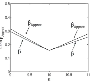
Figure 3:βandβApproxvs.K, whereKr=10, pmin=0.3,m=20,γ=1.
β = 2
γ
1 K
1−(m−1)pmin
m+K
+2
γ|Kr−K|Eζ∼Bin(m−1,pmin)
1 K
ζ m+K−ζ−1
+Kr
m m+K+
1 K
1− ζ
m+K
,
and where Q={x∈
X
:Pz∼D(x∈z)>0}are the items that have some probability of being chosen by the customer. Out of these, any item that is the least likely to be chosen has probability pmin:=minx∈QPz∼D(x∈z).
The stabilityβhas two main terms. The first term decreases generally as 1/K. The second term arises from the error in measuring loss withKrrather thanK. In order to interpretβ, consider the following approximation to the expectation in the bound, which assumes thatmis large and that m≫K≫0, and thatζ≈mpmin:
β≈2 γ
1 K
1−(m−1)pmin
m+K
+2
γ|Kr−K|
1 K pmin
1−pmin+Kr
. (7)
Intuitively, if eitherKis close toKrorpminis large (close to 1) then this term becomes small. Figure 3 shows an example plot ofβand the approximation using (7), which we denote byβApprox.
One can observe that ifKr>K, then both terms tend to improve (decrease) with increasingK. WhenKr<K, then the two terms can compete asKincreases.
4.7 Summary of Bounds
We have provided probabilistic guarantees on performance that show the following: 1) For large m, the association rule-based algorithms have a performance guarantee of the same order as other bounds for supervised learning. 2) For smallm, the minimum support threshold guarantees general-ization (at the expense of possibly removing important rules). 3) The adjusted confidence provides a weaker support threshold, allowing important rules to be used, while still being able to generalize. 4) All generalization guarantees depend on the way the goodness of the algorithm is measured (the choice ofKrin the loss function). 5) Important quantities in the learning process may include: |A|