Submatrix localization via message passing
Bruce Hajek [email protected]
Department of ECE and Coordinated Science Lab University of Illinois at Urbana-Champaign Urbana, IL 61801, USA
Yihong Wu [email protected]
Department of Statistics and Data Science Yale University
New Haven, CT 06520, USA
Jiaming Xu [email protected]
Krannert School of Management Purdue University
West Lafayette, IN 47907, USA
Editor:Qiang Liu
Abstract
The principal submatrix localization problem deals with recovering aK×Kprincipal sub-matrix of elevated meanµin a largen×nsymmetric matrix subject to additive standard Gaussian noise, or more generally, mean zero, variance one, subgaussian noise. This prob-lem serves as a prototypical example for community detection, in which the community corresponds to the support of the submatrix. The main result of this paper is that in the regime Ω(√n) ≤ K ≤ o(n), the support of the submatrix can be weakly recovered (witho(K) misclassification errors on average) by an optimized message passing algorithm ifλ=µ2K2/n, the signal-to-noise ratio, exceeds 1/e. This extends a result by Deshpande
and Montanari previously obtained for K = Θ(√n) and µ= Θ(1).In addition, the algo-rithm can be combined with a voting procedure to achieve the information-theoretic limit of exact recovery with sharp constants for allK≥ n
logn( 1
8e+o(1)). The total running time
of the algorithm isO(n2logn).
Another version of the submatrix localization problem, known as noisy biclustering, aims to recover a K1 ×K2 submatrix of elevated mean µ in a large n1×n2 Gaussian
matrix. The optimized message passing algorithm and its analysis are adapted to the bicluster problem assuming Ω(√ni) ≤ Ki ≤ o(ni) and K1 K2. A sharp
information-theoretic condition for the weak recovery of both clusters is also identified.
Keywords: Submatrix localization, biclustering, message passing, spectral algorithms computational complexity, high-dimensional statistics
1. Introduction
The problem ofsubmatrix detection andlocalization, also known asnoisy biclustering (Har-tigan, 1972; Shabalin et al., 2009; Kolar et al., 2011; Butucea and Ingster, 2013; Butucea et al., 2015; Ma and Wu, 2015; Chen and Xu, 2014; Cai et al., 2017), deals with finding a submatrix with an elevated mean in a large noisy matrix, which arises in many
applica-c
tions such as social network analysis and gene expression data analysis. A widely studied statistical model is the following:
W =µ1C∗11
>
C2∗+Z, (1)
whereµ >0,1C∗1 and1C2∗are indicator vectors of the row and column support setsC
∗
1 ⊂[n1] andC∗
2 ⊂[n2] of cardinalityK1 andK2, respectively, andZ is ann1×n2 matrix consisting of independent standard normal entries. The objective is to accurately locate the submatrix by estimating the row and column support based on the large matrix W.
For simplicity we start by considering the symmetric version of this problem, namely, locating a principal submatrix, and later extend our theoretic and algorithmic findings to the asymmetric case. To this end, consider
W =µ1C∗1>C∗+Z, (2)
where C∗ ⊂[n] has cardinality K and Z is an n×n symmetric matrix with {Zij}1≤i≤j≤n
being mutually independent standard normal. Given the data matrix W, the problem of interest is to recoverC∗. This problem has been investigated in (Deshpande and Montanari, 2015; Montanari et al., 2015; Hajek et al., 2017) as a prototypical example of the hidden community problem,1because the distribution of the entries exhibits a community structure, namely,Wi,j ∼ N(µ,1) if both iand j belong toC∗ and Wi,j ∼ N(0,1) if otherwise.
Assuming thatC∗is drawn from all subsets of [n] of cardinalityKuniformly at random, we focus on the following two types of recovery guarantees.2 Let ξ=1
C∗ ∈ {0,1}n denote
the indicator of the community. Letξb=ξb(A)∈ {0,1}n be an estimator.
• We say that ξbexactly recovers ξ if, as n→ ∞,P[ξ6=ξb]→0.
• We say that ξbweakly recoversξ if, asn→ ∞, d(ξ,ξb)/K →0 in probability, whered
denotes the Hamming distance.
The weak recovery guarantee is phrased in terms of convergence in probability, which turns out to be equivalent to convergence in mean. Indeed, the existence of an estimator satisfying d(ξ,ξb)/K → 0 is equivalent to the existence of an estimator such that E[d(ξ,ξb)] = o(K)
(see (Hajek et al., 2017, Appendix A) for a proof). Clearly, any estimator achieving exact recovery also achieves weak recovery; for bounded K, these two criteria are equivalent.
Intuitively, for a fixed matrix sizen, as either the submatrix sizeKor the signal strength µdecreases, it becomes more difficult to locate the submatrix. A key role is played by the parameter
λ= µ 2K2
n ,
which is the signal-to-noise ratio for classifying an indexiaccording to the statisticP
jWi,j,
which is distributed according to N(µK, n) if i∈ C∗ and N(0, n) if i6∈ C∗. As shown in
1. A slight variation of the model in (Deshpande and Montanari, 2015; Hajek et al., 2017) is that the data matrix therein is assumed to have zero diagonal. As shown in (Hajek et al., 2017), the absence of the diagonal has no impact on the statistical limit of the problem as long as K → ∞, which is the case considered in the present paper.
Appendix A, it turns out that if the submatrix sizeKgrows linearly withn, the information-theoretic limits3 of both weak and exact recovery are easily attainable via thresholding. To see this, note that in the case ofK nsimply thresholding the row sums can provide weak recovery inO(n2) time provided thatλ→ ∞, which coincides with the information-theoretic conditions of weak recovery as proved in (Hajek et al., 2017). Moreover, in this case, one can show that this thresholding algorithm followed by a linear-time voting procedure achieves exact recovery whenever information-theoretically possible. Thus, this paper concentrates on weak and exact recovery in the sublinear regime of
Ω(√n)≤K ≤o(n). (3)
We show that an optimized message passing algorithm provides weak recovery in nearly linear – O(n2logn) – time if λ > 1/e. This extends the sufficient conditions obtained in (Deshpande and Montanari, 2015) for the regime K = Θ(√n) and µ = Θ(1).4 Our algorithm is the same as the message passing algorithm proposed in (Deshpande and Mon-tanari, 2015), except that we find the polynomial that maximizes the signal-to-noise ratio via Hermite polynomials instead of using the truncated Taylor series as in (Deshpande and Montanari, 2015). The proofs follow closely those in (Deshpande and Montanari, 2015), with the most essential differences described at the end of Section 2.
We observe that λ >1/eis much more stringent than λ > 4K n log
n
K, the
information-theoretic weak recovery threshold established in (Hajek et al., 2017). It is an open problem whether any polynomial-time algorithm can provide weak recovery forλ≤1/e. In addition, we show that if λ > 1/e, the message passing algorithm followed by a linear-time voting procedure can provide exact recovery whenever information-theoretically possible. This procedure achieves the optimal exact recovery threshold determined in (Hajek et al., 2017) with sharp constants ifK ≥(1
8e+o(1)) n
logn. See Section 3.1 for a detailed comparison with
information-theoretic limits.
The message passing algorithm is simpler to formulate and analyze for the principal submatrix recovery problem; nevertheless, we show in Section 5 how to adapt the message passing algorithm and its analysis to the biclustering problem. Sharp conditions for exact recovery for the biclustering problem was obtained in (Butucea et al., 2015). We show that calculations in (Butucea et al., 2015) with minor adjustments provide information-theoretic conditions for weak recovery as well. The connection between weak and exact recovery via the voting procedure described in (Hajek et al., 2017) carries over to the biclustering problem.
The analysis of the message passing algorithm is based on the moment method adopted in (Deshpande and Montanari, 2015). When the noise matrixZ is Gaussian, an alternative technique to analyze message passing algorithms is introduced in (Bayati and Montanari, 2011) and generalized by (Javanmard and Montanari, 2013). A distinct advantage of the
3. In this paper, by information-theoretic limits, we mean the sufficient and necessary conditions for at-taining weak or exact recovery by any estimator, regardless of its computational cost.
4. The main results (Theorems 1 and 3) of (Deshpande and Montanari, 2015) assumeµ= Θ(1) but not
moment method in our context is that the Gaussian assumption can be relaxed to a sub-gaussian assumption. Accordingly, we introduce the following assumption.
Assumption 1 Given C∗∈[n] and µ >0, the following holds. W is an n×n symmetric matrix with {Wij}1≤i≤j≤n being mutually independent random variables. Let Zij =Wij −
µI{i,j∈C∗}.Then E[Zij] = 0for all i, j, andvar(Zij) = 1 for (i, j)6∈C∗×C∗.Finally, there
is a constant γ >0 that does not depend on n such that EesZij≤ eγs
2/2
for s∈ R, i.e.
the W’s and Z’s are subgaussian with proxy variance γ.
The variance of a subgaussian random variable is less than or equal to its proxy variance, so Assumption 1 implies γ ≥1,and var(Zij)≤γ for alli, j ∈[n] and all n≥1.Of course,
Assumption 1 holds in the Gaussian case such that theZij are allN(0,1) random variables.
Notation For any positive integer n, let [n] = {1, . . . , n}. For any set T ⊂ [n], let
|T| denote its cardinality and Tc denote its complement. For two sets S, T, let S∆T =
(S\T)∪(T \S) denote the set difference. For an m×n matrix M, let kMk and kMkF denote its spectral and Frobenius norm, respectively. Letσi(M) denote its singular values
ordered decreasingly. For any S ⊂ [m], T ⊂ [n], let MST ∈ R|S|×|T| denote (Mij)i∈S,j∈T
and for m = n abbreviate MS = MSS. For a vector x, let kxk denote its Euclidean
norm. We use standard big O notations, e.g., for any sequences {an} and {bn}, an =
Θ(bn) or an bn if there is an absolute constant c > 0 such that 1/c ≤ an/bn ≤ c. All
logarithms are natural and we use the convention 0 log 0 = 0. Let Φ and Q denote the cumulative distribution function (CDF) and complementary CDF of the standard normal distribution, respectively. For ∈[0,1], define the binary entropy function h(),log1
+
(1−) log1−1 . We say a sequence of eventsEn holds with high probability, if P{En} → 1
asn→ ∞. Denote the Kolmogorov-Smirnov (KS) distance between distributions µ and ν by dKS(µ, ν),supx∈R|µ((−∞, x])−ν((−∞, x])|.
2. Algorithms and main results
To avoid a plethora of factors √1
nin the notation, we describe the message-passing algorithm
using the scaled version
A= √1
nW. (4)
Under Assumption 1, the entriesAij are subgaussian with proxy variance γn, mean 0 or √µn,
and variance 1
n for (i, j)6∈C
∗×C∗.This section presents algorithms and theoretical
guar-antees for the symmetric model (2). Extensions to the asymmetric case for the biclustering problem (1) are given in Section 5.2.
Letf(·, t) :R→Rbe a scalar function for each iterationt. Letθti→j+1 denote the message
transmitted from indexito indexj at iteration t+ 1, which is given by
θi→jt+1 = X
`∈[n]\ {i,j}
with the initial conditions θ0
i→j ≡0. Moreover, let θti+1 denote index i’s belief at iteration
t+ 1, which is given by
θti+1 = X
`∈[n]\{i}
A`if(θt`→i, t). (6)
The form of (5) is inspired by belief propagation algorithms, which have the natural non-backtracking property: the message sent from itoj at timet+ 1 does not depend on the message sent from j toi at time t, thereby reducing the effect of echoes of messages sent by j.
To present an informal derivation of the state evolution equations, which track the asymptotic distributions of the messages, let us postulate the following assumptions: Sup-pose that for each fixedt, asn→ ∞: (a) the empirical distribution of (θt
i :i∈C∗) converges
to N(µt, τt2) and the empirical distribution of (θti :i ∈ [n]\C∗) converges to N(0, τt2); (b)
{θt
i→j} are independent ofA; (c)θi→jt ≈θit. Then it follows from (6) andK =o(n) that for
any i∈C∗,
Eθti+1| {θ`→it :`6=i}
(b)
= X
`∈[n]\{i}
E[A`i]f(θt`→i, t)
= õ
n
X
`∈C∗\{i}
f(θt`→i, t)
(a),(c)
−−−−→n→∞ √λE[f(µt+τtZ, t)],
and for any i∈[n],
var θti+1| {θt
`→i :`6=i}
(b)
= X
`∈[n]\{i}
var(A`i)f(θt`→i, t)2
= 1 n
X
`∈[n]\(C∗∪{i})
f(θt`→i, t)2+o(1) (a),(c)
−−−−→n→∞ Ef(τtZ, t)2
,
whereZrepresents a generic standard normal random variable. Since the conditional means and variances have deterministic limits, those are also the limits of the unconditional means and variances. Therefore, we get the following recursive equations for t≥0:
µt+1=
√
λE[f(µt+τtZ, t)], (7)
τt+1=Ef(τtZ, t)2
, (8)
where the initial conditions areµ0 =τ0 = 0.Following (Deshpande and Montanari, 2015), we call (7) and (8) thestate evolution equations. The heuristic derivation of state evolution equations given above is certainly not rigorous mainly due to the dependency betweenθt
i→j’s
is the non-backtracking property of the message passing rule (5), which has the effect of reducing the dependency between θt
i→j’s andA.
Suppose, for the time being, that message distributions are Gaussian with parameters accurately tracked by the state evolution equations. Then it is reasonable to estimate C∗ by selecting those indices i such that θti+1 exceeds a given threshold. More specifically, classifying an index i based on θit+1 boils down to testing two Gaussian hypotheses with signal-to-noise ratio µt+1
τt+1.This gives guidance for selecting the functionsf(·, t) based onµt and τt to maximize µτtt+1+1. For t = 0 any choice of f is equivalent, so long as f(0,0)> 0.
Without loss of generality, for t ≥ 1, we can assume that the variances are normalized, namely, τt = 1 (e.g., we take f(0,0) = 1 to make τ1 = 1) and choose f(·, t) to be the
maximizer of
max
g {E[g(µt+Z)] : E[g(Z)
2] = 1} (9)
whereZ ∼ N(0,1). By change of measure,E[g(µt+Z)] =E[g(Z)ρ(Z)], where
ρ(x) =dN(µt,1)
dN(0,1)(x) =e
xµt−µ2t/2. (10)
Clearly, the bestg aligns with ρ and we obtain
f(x, t) = p ρ(x)
E[ρ2(Z)]
=exµt−µ2t. (11)
With this optimized f, we have τt≡1 and the state evolution (7) reduces to
µt+1 =
√
λE[f(µt+Z, t)] =
√
λeµ 2 t 2 ,
or, equivalently,
µ2t+1=λeµ2t. (12)
Therefore ifλ >1/e, then (12) has no fixed point and henceµt→ ∞ast→ ∞.
Directly carrying out the above heuristic program, however, seems challenging. To rigorously justify the state evolution equations in Section 6, we rely on the the method of moments, requiringf to be a polynomial, which prompts us to look for the best polynomial of a given degree that maximizes the signal-to-noise ratio. Denoting the corresponding state evolution by (µbt,τbt), we aim to solve the following finite-degree version of (9):
max{E[g(µbt+Z)] : E[g(Z)
2] = 1,deg(g)≤d}. (13) As shown in Lemma 7, this problem can be easily solved via Hermite polynomials, which form an orthogonal basis with respect to the Gaussian measure, and the optimal choice, denoted by fd(·, t),is the best degree-d L2-approximation of the the likelihood ratio (10),
degree which results in the following state evolution that is optimal among all polynomial f of degree d:
b
µ2
t+1 =λ
d
X
k=0
b
µ2k t
k! . (14)
For any λ > 1/e, there is an explicit choice of the degree ddepending only on λ denoted by d∗(λ),5 so that
b
µt → ∞ as t → ∞ and the state evolution (14) for fixed t correctly
predicts the asymptotic behavior of the messages when n → ∞. Therefore, as discussed above, Ce produced by thresholding messages θti, is likely to contain a large portion of C∗,
but sinceK=o(n), it may (and most likely will) also contain a large number of indices not in C∗. Following (Deshpande and Montanari, 2015, Lemma 2.4), we show that the power
iteration6 (a standard spectral method) in Algorithm 1 can remove a large portion of the outlier vertices inC.e
Combining message passing plus spectral cleanup yields Algorithm 1 for estimating C∗ based on the messages θt
i, with theoretical guarantees given in Theorem 1.
Algorithm 1 Message passing
1: Input: n, K ∈N,µ >0,A∈Rn×n,d∗, t∗ ∈N,and s∗ >0.
2: Initialize: θ0i→j = 0 for alli, j ∈[n] withi6=jandθi0= 0. Fort≥0, define the sequence
of degree-d∗ polynomialsfd∗(·, t) as per Lemma 7 and
b
µtin (14).
3: Runt∗−1 iterations of message passing as in (5) with f =fd∗ and computeθt ∗ i for all
i∈[n] as per (6).
4: Find the setCe={i∈[n] :θt
∗
i ≥µbt∗/2}.
5: (Cleanup via power method) Recall that A e
C denotes the restriction of A to the rows
and columns with index in C.e Sample u0 uniformly from the unit sphere in R|C|e and
computeut+1 =A
e
Cu t/kA
e
Cu
tk for 0≤t≤ ds∗logne −1.Let
b
u=uds∗logne.Return
b
C, the set ofK indicesi inCe with the largest values of |ubi|.
Theorem 1 Fix λ > 1/e. Let K and µ depend on n in such a way that µ2K2/n → λ and Ω(√n) ≤ K ≤ o(n) as n → ∞. Suppose either C∗ is deterministic with |C∗| ≡ K,
or C∗ is random such that |C∗|/K → 1 in probability as n → ∞. Suppose Assumption 1 holds for some γ > 0. Let d = d∗(λ) as in (28). For every η ∈ (0,1), there exist explicit positive constantst∗, s∗, cdepending onλ, ηandγ such that Algorithm 1 returns
b
Csatisfying |Cb∆C∗| ≤ηK, with probability converging to one as n→ ∞, and the total time complexity
is bounded by c(η, λ, γ)n2logn, where c(η, λ, γ)→ ∞ as either η→0 or λ→1/e.
Remark 2 Algorithm 1 requires the knowledge of the parameterλto define the sequence of polynomials fd∗(·, t) and
b
µt, and the knowledge of the parameter K in the spectral cleanup
5. See (28) and Remark 9 for the expression.
6. As far as statistical utility is concerned, we could replace ubproduced by the power iteration by the leading singular vector of ACe, but that would incur a higher time complexity because singular value
step. To avoid the need to knowK, we can simply replace the last step of the spectral clean-up (involving choosing theK coordinates of the largest magnitude ofbu) by applyingk-means
with k = 2 on the set {|bui|: i∈ Ce}. See Appendix C for details. With this modification,
Theorem 1 continues to hold as long as λ (or a lower bound thereof ) is known in order to set the degreed∗ and the iteration numbert∗.
Remark 3 As pointed out in (Deshpande and Montanari, 2015, Remeark 2.5), the effective signal-to-noise ratio λcan be potentially improved by a suitable entrywise pre-processing of the observed matrix W. In particular, in (4) we letAij =g(Wij) for some transformation
functiong:R→R. The optimal transformation g in the Gaussian case for whichγ = 1 is
given by the maximizer of
max
g
E[g(µ+Z)]−E[g(Z)] :Eg(Z)2= 1
n
.
In view of (9) and (10), the optimal transformation is the scaled likelihood ratio:
Aij =
1
p
n(eµ2
−1)
dN(µ,1)
dN(0,1)(Wij)−1
= p 1
n(eµ2
−1)
eWijµ−µ2/2−1 and the signal-to-noise ratio λ is increased to
e
λ= K 2 n
eµ2 −1.
If the resultingAij is subgaussian with scaleO(1/n), then Theorem 1 still applies. However,
even if the results extend, in the regime of K √n which we are mostly interested in, we have µ → 0 and eλ=λ(1 +o(1)), and thus pre-processing cannot boost the signal-to-noise
ratio asymptotically.
After the message passing algorithm and spectral cleanup are applied in Algorithm 1, a final linear-time voting procedure is deployed to obtain weak or exact recovery, leading to Algorithm 2 next. As in (Deshpande and Montanari, 2015), we consider a threshold estimator for each vertex ibased on a sum over Cb given by ri =
P
j∈CbAij. Intuitively, ri
can be viewed as the aggregated “votes” received by the index i inCb, and the algorithm
picks the set of K indices with the most significant “votes”. To show that this voting procedure succeeds in weak recovery, a key step is to prove that ri is close to Pj∈C∗Aij.
Ifµ= Θ(1) as in (Deshpande and Montanari, 2015), given that |Cb4C∗|=o(K),the error
incurred by summing over Cb instead of over C∗ could be bounded by truncating Aij to a
large magnitude. However, forµ→0 that approach fails. Our approach is to introduce the clean-up procedure in Algorithm 2 based on the successive withholding method described in (Hajek et al., 2017) (see also (Condon and Karp, 2001; Mossel et al., 2014) for variants of this method). In particular, we randomly partition the set of vertices into 1/δ subsets. One at a time, one subset, say S, is withheld to produce a reduced set of vertices Sc, on
which we apply Algorithm 1. The estimate obtained from Sc is then used by the voting
procedure to classify the vertices inS. The analysis of the two stages is decoupled because conditioned onC∗, the outcome of Algorithm 1 depends only onASc, which is independent
Algorithm 2 Message passing plus voting
1: Input: n, K ∈N,µ >0,A∈Rn×n,δ ∈(0,1) with 1/δ, nδ∈N,d∗, t∗ ∈N,and s∗ >0.
2: Partition [n] into 1/δ subsets Sk of sizenδ randomly.
3: (Approximate recovery) For eachk= 1, . . . ,1/δ, run Algorithm 1 (message passing for
approximate recovery) with input n(1−δ),dK(1−δ)e, µ, ASc k, d
∗, t∗, s∗
which outputs
b
Ck.
4: (Clean up) For each k = 1, . . . ,1/δ compute ri =Pj∈ b
CkAij for all i ∈Sk and return C0, the set ofK indices in [n] with the largest values of ri.
The following theorem provides a sufficient condition for the message passing plus voting cleanup procedure (Algorithm 2) to achieve weak recovery, and, if an additional sufficient condition is also satisfied, exact recovery.
Theorem 4 Suppose K and µ depend on n in such a way that µ2nK2 → λ for some fixed λ >1/e, and Ω(√n)≤K ≤o(n) as n→ ∞.Suppose Assumption 1 holds for some γ >0
and |C∗|=K. Let δ >0 be such that λe(1−δ)>1. Define d∗ =d∗(λ(1−δ)) as per (28). Then there exist positive constantst∗, s∗, c determined explicitly by δ, λ andγ, such that
1. (Weak recovery) Algorithm 2 returns C0 with |C0∆C∗|/K →0 in probability as n→
∞.
2. (Exact recovery) Furthermore, assume that
lim inf
n→∞
√
Kµ
√
2 logK+√2 logn >
√γ. (15)
Let δ >0 be chosen such that for all sufficiently large n,
min
(
λe(1−δ),√ Kµ(1−2δ)
2KγlogK+p2Kγlog(n−K) +δ√K
)
>1.
Then Algorithm 2 returns C0 withP{C0=6 C∗} →0 as n→ ∞.
The total time complexity is bounded byc(δ, λ, γ)n2logn, where c(δ, λ, γ)→ ∞ as δ→0 or λ→1/e.
Remark 5 Theorem 4 ensures Algorithm 2 achieves exact recovery if both (15) andλ >1/e hold; it is of interest to compare these two conditions. Note that
√
Kµ
√
2 logK+√2 logn =
√
λe×
r n
8eKlogn
2 (1 +p
logK/logn).
Hence, if lim infn→∞Klogn/n ≥ 1/(8eγ), then lim infn→∞logK/logn = 1; thus (15)
implies λ > 1/e and hence (15) alone is sufficient for Algorithm 2 to succeed. If instead
lim supn→∞Klogn/n ≤ 1/(8eγ), then λ > 1/e implies (15) and thus λ > 1/e alone is
Montanari, 2015) entails K = Θ(√n),in which case the condition λ >1/eis sufficient for exact recovery, as shown in (Deshpande and Montanari, 2015). The idea of upgrading weak recovery to exact recovery via a local voting procedure has also appeared in (Abbe et al., 2016; Mossel et al., 2015; Abbe and Sandon, 2015; Yun and Proutiere, 2015) under the context of stochastic block models with community sizes scaling linearly in n. As shown in (Hajek et al., 2017, Corollary 4) in the Gaussian case for which γ = 1, the condition (15), with strict inequality replaced by greater than or equal, is necessary for exact recovery.
We finish this section by discussing the connections and distinctions to the previous work (Deshpande and Montanari, 2015). Versions of Theorems 1 and 4 are given in (Deshpande and Montanari, 2015) for the case K = Θ(√n) and µ = Θ(1). We extend the range of K to Ω(√n) ≤ K ≤ o(n), showing that the message passing plus a cleanup procedure achieves the optimal exact recovery threshold in the Gaussian case with sharp constants if K ≥(81e +o(1))lognn. The algorithms and proofs are nearly the same; we comment here on the main difficulties we encountered when allowing K/√n→ ∞ and µ→0.
First, a key ingredient in the proof of Theorem 1 is Lemma 6. Its proof is based on the moment method and a largerK requires modification of bounds from (Deshpande and Montanari, 2015) used in calculating the moments of messages, i.e., E
h
(θt i→j)m
i
for fixed m∈N, by a more careful counting argument. We refer the interested readers to Remark 31
right after the proof of Lemma 6 for more details.
Secondly, after the message passing algorithm and spectral cleanup are applied in Al-gorithm 1, a final cleanup procedure is applied to obtain weak recovery or exact recovery (when possible). As in (Deshpande and Montanari, 2015), we consider a threshold estima-tor for each vertexibased on a sum overC.b IfK = Θ(
√
n) as assumed in (Deshpande and Montanari, 2015), then λbeing a constant implies that the mean µis bounded away from zero. In this case if|Cb4C∗|=o(K),the error incurred by summing over Cb instead of over
C∗ could be bounded by truncatingAij to a large magnitude ¯ρand bounding the difference
of sums by ¯ρ C∗4Cb
=o(K)µK.However, forK √
nwith vanishingµthis approach fails. Instead, we rely on the cleanup procedure in Algorithm 2 which entails running Al-gorithm 1 for 1/δ times on subsampled vertices. A related difference we encounter is that if K is large enough then the condition λ > 1/e alone is not sufficient for exact recovery, but adding the information-theoretic condition (15) suffices.
Lastly, the method of moments requiresf(·, t) to be a polynomial so that the exponential function (11), which results in the ideal state evolution (12), cannot be directly applied. It is shown in (Deshpande and Montanari, 2015, Lemma 2.3) that for any λ > 1/e and any thresholdM there existsd∗=d∗(λ, M) so that takingf to be the truncated Taylor series of (11) up to degreed∗ results in the state evolutionbµtwhich exceedsM after some finite time
t∗(λ, M); however, no explicit formula of d∗, which is needed to instantiate Algorithm 1,
3. Statistical optimality and computational considerations
3.1 Comparison with information-theoretic limits in the Gaussian case
As noted in the introduction, in the regime K = Θ(n), a thresholding algorithm based on row sums provides weak and, if a voting procedure is also used, exact recovery whenever it is informationally possible in the Gaussian case. In this subsection, we compare the performance of the message passing algorithms to the information-theoretic limits on the recovery problem in the regime (3). Throughout this section we restrict attention to the Gaussian case, such that Zij ∼ N(0,1) and γ = 1. Also, for converse results, we assume
the true community C∗ is a subset of [n] of cardinality K selected uniformly at random. Notice that the comparison here takes into account the sharp constant factors. Information-theoretic limits for the biclustering problem are discussed in Section 5.1.
Weak recovery The information-theoretic threshold for weak recovery has been deter-mined in (Hajek et al., 2017, Theorem 2), which, in the regime of (3), boils down to the following: If
lim inf
n→∞
Kµ2
4 logKn >1, (16)
then weak recovery is possible; conversely, if weak recovery is possible, then
lim inf
n→∞
Kµ2
4 logKn ≥1. (17)
This implies that the minimal signal-to-noise ratio for weak recovery is
λ≥(4 +)K n log
n K
for any >0, which vanishes in the sublinear regime ofK=o(n). In contrast, in the regime of (3), message passing (Algorithm 1) demands a non-vanishing signal-to-noise ratio, namely, λ > 1/e, to achieve weak recovery. No polynomial-time algorithm is known to succeed if λ ≤ 1/e, suggesting that computational complexity might incur a severe penalty on the statistical optimality when K=o(n).
Exact recovery When the submatrix size satisfies (3), if (15) with γ = 1 holds, then exact recovery is possible; conversely, if exact recovery is possible, then
lim inf
n→∞
√
Kµ
√
2 logK+√2 logn ≥1. (18)
See (Hajek et al., 2017, Corollary 4). This implies that the minimal signal-to-noise ratio for exact recovery is
λ≥(2 +)K n
p
logn+plogK2 (19) for any > 0. Consequently, we find that the critical submatrix size for which message passing (plus cleanup) can achieve optimal exact recovery is n
• K = ωlognn. In this regime, the right hand side of (19) goes to ∞ and hence the minimal signal-to-noise ratio for exact recovery is much higher than that of weak recovery via message passing, namely, 1/e. Thus, exact recovery can be attainable in polynomial-time by message-passing plus voting clean-up (Algorithm 2).
• K = Θ(lognn). In this regime, if we letK = logρnn, the right hand side of (19) is at least 1/eifρ≥ 1
8e and strictly less than 1/eotherwise. In view of Theorem 4, we conclude
that message passing plus voting cleanup (Algorithm 2) achieves the sharp threshold of exact recovery if
K≥
1
8e +o(1)
n
logn. (20)
• K = olognn. In this regime, the right hand side of (19) is o(1). No polynomial-time algorithm (including semidefinite programming relaxation (Hajek et al., 2016)) is known to achieve weak, let alone exact, recovery, whenλ=o(1).
A counterpart of this conclusion for the biclustering problem is obtained in Remark 20 in terms of the submatrix sizes.
3.2 Comparison with the spectral limit
It is reasonable to conjecture that λ >1 is the spectral limit for recoverability by spectral estimation methods. This conjecture is rather vague, because it is difficult to define what constitutes spectral methods. Nevertheless, some evidence for this conjecture is provided by (Deshpande and Montanari, 2015, Proposition 1.1), which, in turn, is based on results on the spectrum of a random matrix perturbed by adding a rank-one deterministic matrix (Knowles and Yin, 2013, Theorem 2.7).
The message passing framework used in this paper itself provides some evidence for the conjecture. Indeed, if f(x,0) ≡ 1 and f(x, t) = x for all t ≥ 1, the iterates θt are
close to what is obtained by iterated multiplication by the matrixA,beginning with the all one vector, which is the power method for computation of the eigenvector corresponding to the principal eigenvalue of A.7 To be more precise, with this linear f the message passing equation (5) can be expressed in terms of powers of the non-backtracking matrix B∈R(
n 2)×(
n
2) associated with the matrixA, defined byBef =Ae
1,e21{e2=f1}1{e16=f2}, where e = (e1, e2) and f = (f1, f2) are directed pairs of indices. Let Θt ∈
Rn(n−1) denote the
messages on directed edges with Θt
e = θte1→e2. Then, (5) simply becomes Θ
t = Bt1. To
evaluate the performance of this method, we turn to the state evolution equations (7) and (8), which yield µt = λt/2 and τt = 1 for all t ≥ 1. Therefore, by a simple variation of
Algorithm 1 and Theorem 1, if λ > 1, the linear message passing algorithm can provide weak recovery.
For the submatrix detectionproblem, namely, testing µ= 0 (pure noise) versus µ >0, as opposed to support recovery, if λ is fixed with λ > 1, a simple thresholding test based
7. If we includedi, j in the summation in (5) and (6), then we would haveθt =At1exactly. Since the entries ofAareOP(1/
√
on the largest eigenvalue of the matrixAprovides detection error probability converging to zero (F´eral and P´ech´e, 2007), while if λ < 1 no test based solely on the eigenvalues of A can achieve vanishing probability of error (Montanari et al., 2015). It remains, however, to establish a solid connection between the detection and estimation problem for submatrix localization for spectral methods.
3.3 Computational barriers in the Gaussian case
A recent line of work (Kolar et al., 2011; Ma and Wu, 2015; Chen and Xu, 2014; Cai et al., 2017) has uncovered a fascinating interplay between statistical optimality and com-putational efficiency for the recovery problem and the related detection and estimation
problem.8 Assuming the hardness of the planted clique problem, rigorous computational lower bounds have been obtained in (Ma and Wu, 2015; Cai et al., 2017) through reduction arguments in the Gaussian case. In particular, it is shown in (Ma and Wu, 2015) that when K = nα for 0 < α < 2/3, merely achieving the information-theoretic limits of
de-tection within any constant factor (let alone sharp constants) is as hard as detecting the planted clique; the same hardness also carries over to exact recovery in the same regime. Furthermore, it is shown that the hardness of estimating this type of matrix, which is both low-rank and sparse, highly depends on the loss function (Ma and Wu, 2015, Section 5.2). For example, for K = Θ(√n), entry-wise thresholding attains an O(logn) factor of the minimax mean-square error; however, if the error is gauged in squared operator norm in-stead of Frobenius norm, attaining an O(√n/logn) factor of the minimax risk is as hard as solving planted clique. Similar reductions have been shown in (Cai et al., 2017) for exact recovering of the submatrix of sizeK =nαand the planted clique recovery problem for any
0< α <1.
The results in (Ma and Wu, 2015; Cai et al., 2017) revealed that the difficulty of sub-matrix localization crucially depends on the size and planted clique hardness kicks in if K =n1−Θ(1). In search of the exact phase transition point where statistical and computa-tional limits depart, we further zoom into the regime ofK =n1−o(1). We showed in (Hajek et al., 2016) no computational gap exists in the regimeK=ω(n/logn), since a semidefinite programming relaxation of the maximum likelihood estimator can achieve the information limit for exact recovery with sharp constants. The current paper further pushes the bound-ary toK ≥ n
logn(
1
8e +o(1)), in which case the sharp information limits can be attained in
nearly linear-time via message passing plus clean-up. However, as soon asK ≤ n
logn(
1 8e−)
for any > 0, a gap emerges between the statistical limits and the sufficient condition of message passing plus clean-up, given byλ >1/e.
4. Proofs of algorithm correctness
We first justify the state evolution equations via the following key lemma, which establishes the asymptotic normality of the empirical distribution of messages with mean and variance given by (7) and (8). A version of this lemma is proved in (Deshpande and Montanari,
2015) by assuming µ = Θ(1) and K = Θ(√n). The proof is given in Section 6 using the method of moments, closely following (Deshpande and Montanari, 2015).
Lemma 6 Let f(·, t) be a finite-degree polynomial for each t≥0. Let K and µ depend on nsuch that K2nµ2 ≡λfor someλ >0 andΩ(√n)≤K≤o(n).Suppose Assumption 1 holds for some γ > 0, and suppose either C∗ is deterministic with |C∗| ≡ K, or C∗ is random
such that|C∗|/K→1 in probability asn→ ∞.Let A=W/√n and setθ0
i→j = 0. Consider
the message passing algorithm defined by (5) and (6). Then for each fixed t, as n→ ∞,
dKS 1
|C∗|
X
i∈C∗
δθt
i, N(µt, τ 2
t)
!
p
→0,
dKS
1 n− |C∗|
X
i /∈C∗
δθt
i, N(0, τ 2
t)
!
p
→0,
where µt andτt are defined in (7) and (8), respectively; |C1∗|
P
i∈C∗δθt i and
1
n−|C∗|
P
i /∈C∗δθt i are the empirical distributions of θt
i for i∈C∗ and i /∈C∗, respectively.
Next we prove Theorems 1-4. Lemma 6 implies that if i ∈C∗, thenθt
i ∼ N(µt, τt2); if
i /∈ C∗, then θt
i ∼ N(0, τt2). Ideally, one would pick the optimal f(x, t) = eµt(x−µt) which
result in the optimal state evolutionµt+1 =
√
λeµ2
t/2 and τt= 1 for allt≥1. Furthermore,
ifλ >1/e, then µt→ ∞as t→ ∞, and thus we can hope to estimate C∗ by selecting the
indices isuch that θt
i exceeds a certain threshold. The caveat is that Lemma 6 needs f to
be a polynomial of finite degree. Next we proceed to find the best degree-dpolynomial for iterationt, denoted by fd(·, t), which maximizes the signal to noise ratio.
Recall that the Hermite polynomials{Hk:k≥0} are the orthogonal polynomials with
respect to the standard normal distribution (cf. (Szeg¨o, 1975, Section 5.5)), given by
Hk(x) = (−1)k
ϕ(k)(x) ϕ(x) =
bk/2c
X
i=0
(−1)i(2i−1)!!
k 2i
xk−2i, (21)
whereϕdenotes the standard normal density andϕ(k)(x) is itsk-th derivative; in particular, H0(x) = 1, H1(x) = x, H2(x) =x2−1. Furthermore, deg(H
k) =k and {H0, . . . , Hd} span
all polynomials of degree at most d. For Z ∼ N(0,1), E[Hm(Z)Hn(Z)] = m!δm=n and
E[Hk(µ+Z)] = µk for all µ∈ R; hence the relative density ddNN((0µ,,1)1)(x) =eµx−µ2/2 admits
the following expansion:
eµx−µ2/2 =
∞
X
k=0 Hk(x)
µk
k!. (22)
Truncating and normalizing the series at the firstd+1 terms immediately yields the solution to (13) as the best degree-d L2-approximation to the relative density, described as follows: Lemma 7 Fix d∈N and defineµbt according to the iteration (14) with µb0= 0, namely,
b
µ2t+1 =λGd(µb
2
t), Gd(µ) = d
X
k=0 µk
Define
fd(x, t) = d
X
k=0
akHk(x), (24)
where ak , µb
k t
k!(
Pd
k=0
b
µ2k t
k! )
−1/2. Then f
d(·, t) is the unique maximizer of (13) and the state
evolution (7) and (8) with f =fd coincides with τt= 1 and µt=µbt. Furthermore, for any
d≥2 the equation
Gd(a) =aGd−1(a) (25) has a unique positive solution, denoted by a∗
d. Let
λ∗d= 1 Gd−1(a∗d)
(26)
and defineλ∗
1 = 1. Then
1. for any d∈N and any λ > λ∗d, µbt→ ∞ as t→ ∞ and hence for any M >0,
t∗(λ, M) = inf{t:µbt> M} (27)
is finite;
2. λ∗d↓1/e monotonically as d→ ∞ according to λd∗= 1/e+ 1/e(d2+1)!+o(1).
Remark 8 The best affine update givesλ∗1= 1; for the best quadratic update,a∗2 =√2and hence λ∗
2 = 1+1√2 ≈0.414. More values of the threshold are given below, which converges to 1/e≈0.368rapidly.
d 1 2 3 4 5
λ∗
d 1 0.414 0.376 0.369 0.368
Remark 9 Let
d∗(λ) = inf{d∈N:λ∗d< λ}, (28)
which is finite for any λ >1/e. Then for anyd≥d∗,
b
µt→ ∞ as t→ ∞. As λapproaches
the critical value1/e, the degreed∗(λ)blows up according tod∗(λ) = Θ(logλe−1 1/log logλe−1 1), as a consequence of the last part of Lemma 7.
Remark 10 (Best affine message passing) Ford= 1, the best state evolution is given by
b
µ2t+1 =λ(1 +µb
2
t)
and the corresponding optimal update rule is
f1(x, t) = 1 +bµtx p
1 +bµ
2
t
.
This is strictly better than f(x, t) = x described in Section 3.2 which gives µb
2
t+1 = λµb
2
t;
Proof [Proof of Lemma 7] Note that any degree-dpolynomial gcan be written in terms of the linear combination:
fd(x, t) = d
X
k=0
ckHk(x),
where the coefficients {ck} satisfy E[g2(Z)] = Pdk=0k!c2k = 1. By a change of measure,
E[g(µbt+Z)] = E[g(Z)e b
µtZ−µb
2
t/2] = Pd
k=0ckµb
k
t, in view of the orthogonal expansion (22).
Thus, to solve the maximization problem (13), it is equivalent to solving
max
ck
( d X
k=0 ckbµ
k t :
d
X
k=0
k!c2k= 1
)
.
By Cauchy-Schwarz inequality, the optimal coefficients and the optimal polynomialfd(·, t)
are given by (24), resulting in the following state evolution
b
µt+1=
√
λmax{E[g(µbt+Z)] : E[g(Z)
2] = 1,deg(g)≤d}= λ
d
X
k=0
b
µ2k t
k!
!1/2
,
which is equivalent to (23).
Next we analyze the behavior of the iteration (23). The case of d= 1 follows from the obvious fact that µb2
t+1 =λ(µb
2
t + 1) diverges if and only if λ≥1. For d≥2, note that Gd
is a strictly convex function withGd(0) = 1 andG0d=Gd−1. Also, (Gd(a)−aGd−1(a))0 =
−aG00d(a)<0. Thus,Gd(a)−aGd−1(a) is strictly decreasing ona >0 with value d1! ata= 1 and limit −∞ asa→ ∞,so (25) has a unique positive solution a∗
d and it satisfiesa∗d>1.
Furthermore, (Gd(a)−aGd−1(a))0
a=1=−
Pd−2
k=0 1
k!,so by Taylor’s theorem, Gd(a)−aGd−1(a) =
1
d!−(a−1)
d−2
X
k=0 1
k!+O((a−1) 2),
yielding
a∗d= 1 + 1 d!Pd−2
k=0 1
k!
+O(1/(d!)2).
Consider next the values ofλsuch that bµt diverges. For very largeλ,Gd(a) dominates a/λ
pointwise andµbtdiverges. The critical value ofλis whenGd(a) anda/λmeet tangentially,
namely,
λGd−1(a) = 1, λGd(a) =a,
whose solution is given bya=a∗d and λ=λ∗d,where
λ∗d, 1
Gd−1(a∗d)
= 1
Gd−1(1) +G0d−1(1)(a
∗
d−1) +O((a ∗ d−1)2)
= 1
Pd
k=0k1!+O(1/(d!)2)
= 1/e+
P∞
k=d+11/k! +O(1/(d!)2) ePd
k=01/k! = 1/e+ 1/e
Thus,λ∗
d is the minimum value such that for all λ > λ∗d,λGd(a)> a for all a >0, so that
starting from any µbt ≥0 we have µbt → ∞ monotonically. The fact λ
∗
d is decreasing in d
follows from the fact Gdis pointwise increasing in d.
Lemmas 6 and 7 immediately imply the following partial recovery results.
Lemma 11 Assume that λ > 1/e and Ω(√n) ≤ K ≤ o(n). Fix any ∈ (0,1). Let M = p8 log(1/) and run the message passing algorithm for t iterations with f = fd∗,
d∗ =d∗(λ) as in (28), and t=t∗(λ, M) as in (27). Let Ce ={i:θt
∗
i ≥µbt∗/2}. Then with
probability converging to one as n→ ∞,
1
K|Ce∩C
∗
| ≥1− (29)
K(1−)≤ |Ce| ≤n. (30)
Proof Notice that
|Ce∩C∗|= X
i∈C∗
1{θt∗
i ≥µbt∗/2}
.
By the choice of f =fd in (24), we have τt= 1 for allt≥1. It follows from Lemma 6 that
lim
n→∞
1
K|Ce∩C
∗
|=P{µbt∗+Z ≥µbt∗/2}, (31)
where the convergence is in probability. Notice that we have usedd=d∗(λ) andt=t∗(λ, M)
defined by (28) and (27) in Lemma 7. Thusµbt∗ ≥M = p
8 log(1/) and
P{µbt∗+Z ≤µbt∗/2}=Q(µbt∗/2)≤e
−µb2
t∗/8≤,
which, in view of (31), implies (29) with probability converging to one asn→ ∞.Similarly, Lemma 6 implies that in probability
lim
n→∞
1 n|Ce\C
∗
|=P{Z≥µbt∗/2}=Q(µbt∗/2)≤. (32)
Since K=o(n), we haveP{K(1−)≤ |Ce| ≤n} →1.
AlthoughCe contains a large portion ofC∗, since|Ce|is linear innwith high probability,
i.e.,|Ce|/n→Q(µbt∗/2) by Lemma 6, it is bound to contain a large number of outlier indices.
The next lemma, closely following (Deshpande and Montanari, 2015, Lemma 2.4), shows that given the conclusion of Lemma 11, the power iteration in Algorithm 1 can remove most of the outlier indices inC.e Its proof is presented in Appendix B.
Lemma 12 Suppose λ = µ2nK2 ≥ 1/e, K → ∞, |C∗|/K → 1 in probability, and Ce is
a set (possibly depending on A) such that (29) – (30) hold for some 0 < < 0, where 0< 0≤1/2 is determined by 1−0 = 8ep4γh(0) + 10γ0. Let
s∗ = 2
log(√λ(1−)/(8p
where h(),log1
+ (1−) log
1
1− is the binary entropy function. ThenCb with |Cb| ≡K
produced by Algorithm 1 returns |Cb∆C∗| ≤ η(, λ, γ)K, with probability converging to one
as n→ ∞,where
η(, λ, γ) = 2+eγ4608h() + 11520
λ(1−)2 . (34) Proof [Proof of Theorem 1] Given η ∈ (0,1), choose an arbitrary ∈ (0, 0) such that η(, λ, γ) defined in (34) is at most η. With t∗ specified in Lemma 11 and s∗ specified in Lemma 12, the probabilistic performance guarantee in Theorem 1 readily follows by com-bining Lemmas 11 and 12. The time complexity of Algorithm 1 follows from the fact that for both the BP algorithm and the power method each iteration has complexityO(n2) and Algorithm 1 entails running BP and the power method for t∗ and ds∗logne iterations re-spectively; both t∗ and s∗ are constants depending only onη, λ, andγ.
Proof[Proof of Theorem 4] (Weak recovery) Fixk∈[1/δ] and letCk∗ =C∗∩Sc
k.Define the
n(1−δ)×n(1−δ) matrixAk,ASc
k, which corresponds to the submatrix localization problem
for a planted community C∗
k whose size has a hypergeometric distribution, resulting from
sampling without replacement, with parameters (n, K,(1−δ)n) and mean (1−δ)K.By a result of (Hoeffding, 1963), the distribution of|Ck∗|is convex order dominated by the distri-bution that would result from sampling with replacement, namely, the Binom n(1−δ),K
n
distribution. In particular, Chernoff bounds for Binom(n(1−δ),K
n) also hold for |C ∗ k|,so
|C∗
k|/((1−δ)K) → 1 in probability as n → ∞. Note that
((1−δ)K)2µ2
n(1−δ) → λ(1−δ) and λ(1−δ)e >1 by the choice of δ.Letd∗(λ(1−δ)) be given in (28), i.e.,
d∗(λ(1−δ)) = inf{d∈N:λ∗d< λ(1−δ)}.
Choose an arbitrary∈(0, 0) to satisfyη(, λ(1−δ), γ)≤δ, i.e., 2+eγ4608h() + 11520
λ(1−δ)(1−)2 ≤δ.
Define µbtrecursively according to (14) withλreplaced by λ(1−δ) andµ0b = 0, i.e.,
b
µ2
t+1 =λ(1−δ)
d
X
k=0
b
µ2k t
k! .
Define t∗(δ, λ, γ) according to (27) with M = 8 log(1/), and s∗(δ, λ, γ) according to (33) with λ replaced by λ(1−δ). Then Theorem 1 with n and K replaced by n(1−δ) and
dK(1−δ)e implies that asn→ ∞,
P
n
|Cbk4Ck∗| ≤δK for 1≤k≤1/δ o
→1.
Given (C∗
k,Cbk), each of the random variables ri √
n fori∈Sk is conditionally subgaussian
with proxy variance at mostKγ. Furthermore, on the event,Ek={|Cbk4Ck∗| ≤δK},
Therefore, on the event Ek, for i ∈ Sk ∩C∗, ri√n has mean greater than or equal to
K(1−2δ)µ, and for i∈Sk\C∗,ri has mean zero.
Define the following set by thresholding
Co0 ={i∈[n] :ri ≥(1−2δ)
√
λ/2}
The number of indices in Sk incorrectly classified byCo0 ∩Sk satisfies (use |Sk|=δn):
E(Co0 ∩Sk)∆(C∗∩Sk)
≤δne−Ω(n/K),
where the last inequality follows because ri is subgaussian with proxy variance at most
γK/n. Summing overk∈[1/δ] yieldsE[|Co0∆C∗|]≤ne−Ω(n/K).By Markov’s inequality,
P|Co0∆C ∗
| ≥K2/n ≤ n
2 K2e
−Ω(n/K) K==o(n)o(1).
Instead of C0
o, Algorithm 2 outputs C0 which selects the K indices in [n] with the largest
values ofri.Applying the same argument as that at the end of the proof of Lemma 12, we
get|C∗4C0| ≤2|C∗4Co0|+||C∗| −K|,and hence |C∗4C0|/K →0 in probability.
(Exact recovery) By the union bound and Chernoff’s bound for subgaussian random variables, the maximum ofm subgaussian random variables Xi with zero mean and proxy
variance at mostγ satisfies that
P
max 1≤i≤mXi≥
√γp
2 logm+t
≤mexp
−p2 logm+t2/2
= exp−tp2 logm−t2/2.
It follows that max1≤i≤mXi is at most√2γlogm+oP(1) as m → ∞. Also, for k∈[1/δ],
|Sk∩C∗| ≤ |C∗|=K and |Sk\C∗| ≤ |[n]\C∗|=n−K.Therefore,
min
i∈Sk∩C∗
ri√n ≥ K(1−2δ)µ−
p
2KγlogK+oP(
√
K) (35)
max
j∈Sk\C∗
ri√n ≤
p
2Kγlog(n−K) +oP(
√
K). (36)
Since kranges over a finite number of values, namely, [1/δ], (35) and (36) continue to hold with left-hand sides replaced by mini∈C∗ri√n and maxj /∈C∗ri√n, respectively. Therefore,
by the choice ofδ, mini∈C∗ri√n >maxj∈[n]\C∗ri√n with probability converging to one as
n→ ∞ and so C0 =C∗ with probability converging to one as well.
(Time complexity) The running time of Algorithm 2 is dominated by invoking Algorithm 1 for a constant number, 1/δ, of times, and the number of iterations within Algorithm 1 is (t∗ +s∗logn)n2, with both t∗ and s∗ → ∞ as either δ → 0 or λ→ 1/e. In particular,
5. The Gaussian biclustering problem
We return to the biclustering problem where the goal is to locate a submatrix whose row and column support need not coincide. Consider the model (1) parameterized by (n1, n2, K1, K2, µ) indexed by a common n with n → ∞. In Section 5.1 we present the information limits for weak and exact recovery for the Gaussian bicluster model. The sharp conditions given for exact recovery are from (Butucea et al., 2015), and calculations from (Butucea et al., 2015) with minor adjustment provide conditions for weak recovery as well. Section 5.2 shows how the optimized message passing algorithm and its analysis can be extended from the symmetric case to the asymmetric case for biclustering and compares its performance to the fundamental limits. As originally observed in (Hajek et al., 2017) for recovering the principal submatrix, the connection between weak and exact recovery via the voting procedure extends to the biclustering problem as well. Note that for the sake of simplicity, we focus on Gaussian biclustering where the noise matrix Z is Gaussian; the results can be readily extended to the case where Z has subguassian entries as we did in the symmetric case.
5.1 Information-theoretic limits for Gaussian biclustering
Information-theoretic conditions ensuring exact recovery of both C1∗ and C2∗ by the maxi-mum likelihood estimator (MLE), i.e.,
(Cb1MLE,Cb2MLE) = arg max
|C1|=K1
|C2|=K2
X
i∈C1
j∈C2 Wij
are obtained in (Butucea et al., 2015). While (Butucea et al., 2015) does not focus on conditions for weak recovery, the calculations therein combined with the voting procedure for exact recovery described in (Hajek et al., 2017) in fact resolve the information limits for both weak and exact recovery in the bicluster Gaussian model. Throughout this section we assume that Ki =o(ni) for i= 1,2. For the converse results we assume Ci∗ is a subset of
[ni] of cardinalityKi selected uniformly at random for i= 1,2, withC1∗ independent ofC2∗. Let
λi =
K2
iµ2
ni
, fori= 1,2.
Theorem 13 (Weak recovery thresholds for Gaussian biclustering) If
lim inf
n→∞
µ√K1K2
p
2(K1log(n1/K1) +K2log(n2/K2))
>1, (37)
then both C∗
1 and C2∗ can be weakly recovered by the MLE. Conversely, if both C1∗ and C2∗ can be weakly recovered by some estimator, then
lim inf
n→∞
µ√K1K2
p
2(K1log(n1/K1) +K2log(n2/K2)
If C∗
2 (C1∗) can be weakly recovered, one can further obtain exact recovery ofC1∗ (C2∗) via a voting cleanup procedure similar to Algorithm 2; it uses the method of successive withholding. We give the voting procedure in Algorithm 3 for exact recovery of C1∗ based on weak recovery of C∗
2; exact recovery ofC2∗ based on weak recovery ofC1∗ is analogous. Algorithm 3 Weak recovery ofC∗
2 plus cleanup for exact recovery of C1∗ 1: Input: n1, n2, K1, K2∈N,µ >0, A∈Rn1×n2,δ ∈(0,1) with 1/δ, n1δ∈N.
2: (Partition) Partition [n1] into 1/δ subsetsSk of size n1δ randomly.
3: (Approximate recovery) For eachk = 1, . . . ,1/δ, let Ak denote the restriction of A to
the rows with index in Sc
k,run an estimator capable of weak recovery ofC ∗
2 with input (n1(1−δ), n2,dK1(1−δ)e, K2, µ, Ak) which outputs Cb2k.
4: (Clean up) For eachk= 1, . . . ,1/δ compute ri =Pj∈ b
C2kAij for all i∈Sk and return C10, the set ofK indices in [n1] with the largest values ofri.
Theorem 14 (Exact recovery thresholds for Gaussian biclustering) If for some small δ >0, C∗
2 can be weakly recovered even if a fraction δ of the rows of the matrix are hidden, and if
lim inf
n→∞
√
K2µ
√
2 logK1+√2 logn1
>1, (39)
then C1∗ can be exactly recovered by the voting procedure. Conversely, if C1∗ can be exactly recovered by some estimator, then
lim inf
n→∞
√
K2µ
√
2 logK1+√2 logn1 ≥
1. (40)
Similarly, if for some smallδ >0, C1∗ can be weakly recovered even if a fractionδ of the columns of the matrix are hidden, and if
lim inf
n→∞
√
K1µ
√
2 logK2+√2 logn2
>1, (41)
then C2∗ can be exactly recovered by the voting procedure. Conversely, if C2∗ can be exactly recovered by some estimator, then
lim inf
n→∞
√
K1µ
√
2 logK2+√2 logn2 ≥
1. (42)
Corollary 15 If (37), (39), and (41) hold, then C∗
1 and C2∗ can both be exactly recovered by the MLE. Conversely, if exact recovery is possible, then (38), (40), and (42) hold.
We conclude this subsection with a few remarks on Theorems 13 and 14:
1. If n1 = n2 and K1 = K2, the sufficient conditions and the necessary conditions for weak and for exact recovery, respectively, are identical to those in (Hajek et al., 2017) for the recovery of aK×K principal submatrix with elevated mean, in a symmetric n×n Gaussian matrix. Basically, in the bicluster problem the data matrix provides roughly twice the information (because the matrix is not symmetric) and there is twice the information to be learned, namely C∗
1 and C2∗ instead of onlyC∗, and the factors of two cancel to yield the same conditions. It therefore follows from (Hajek et al., 2017, Remark 7), that if n1 =n2 and K1 =K2 ≤n11/9, then (37) implies (39) and (41); in this regime, (37) alone is the sharp condition for both weak and exact recovery.
2. If λi = K
2 iµ2
ni are two fixed positive constants and ifK1 K2,then (37) holds for all
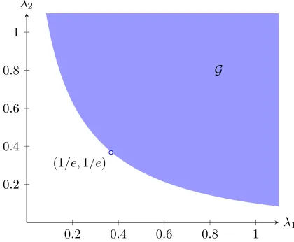
sufficiently largen, so weak recovery is information theoretically possible. In contrast, our proof that the optimized message passing algorithm provides weak recovery in this regime requires (λ1, λ2)∈ G,where G is defined in (52) in the next subsection. 5.2 Message passing algorithm for the Gaussian biclustering model
Supposeni→ ∞and Ω(√ni)≤Ki ≤o(ni) fori∈ {0,1},asn→ ∞.The belief propagation
algorithm and our analysis of it for recovery of a single set of indices can be naturally adapted to the biclustering model.
Let f(·, t) : R → R be a scalar function for each iteration t. To be definite, we shall
describe the algorithm such that at each iteration, the messages are passed either from the row indices to the column indices, or vice-versa, but not both. The messages are defined as follows for t≥0 :
(teven) θi→jt+1 = √1 n2
X
`∈[n2]\{j}
Wi`f(θt`→i, t), ∀i∈[n1], j ∈[n2] (43)
(todd) θj→it+1 = √1 n1
X
`∈[n1]\{i}
W`jf(θt`→j, t), ∀j∈[n2], i∈[n1], (44)
with the initial condition θ0
`→i = 0 for (`, i) ∈ [n2]×[n1]. Moreover, let the aggregated beliefs be given by
(teven) θt+1
i =
1
√n2 X
`∈[n2]
Wi`f(θt`→i, t), ∀i∈[n1] (45)
(todd) θjt+1 = √1 n1
X
`∈[n1]
W`jf(θt`→j, t), ∀j∈[n2]. (46)
Recall λi = K
2 iµ2
ni fori= 1,2.Suppose as n→ ∞, fort even (odd), θ
t
i is approximately
the symmetric case, the update equations of message passing and the fact that θt
i→j ≈ θit
for all i, j suggest the following state evolution equations fort≥0:
µt+1=
(√
λ2E[f(µt+τtZ, t)] teven
√
λ1E[f(µt+τtZ, t)] todd
(47)
τt+1=Ef(τtZ, t)2
. (48)
The optimal choice of f for maximizing the signal-to-noise ratio µt+1
τt+1 is again f(x, t) = exµt−µ2t. With this optimizedf, we haveτt+1= 1 and the state evolution equations reduce
to
µ2t+1 =
(
λ2eµ 2
t t even λ1eµ2
t t odd (49)
withµ0 = 0.
To justify the state evolution equations, we rely on the method of moments, requiring f to be polynomial. Thus, we choose f = fd(·, t) as per Lemma 7, which maximizes the
signal-to-noise ratio among all polynomials with degree up to d. With f = fd, we have
τt+1= 1 and the state evolution equations reduce to
b
µ2t+1 =
(
λ2Gd(µb
2
t) t even
λ1Gd(µb
2
t) t odd
(50)
whereGd(µ) =Pdk=0
µk
k!.
Combining message passing with spectral cleanup, we obtain the following algorithm for estimatingC1∗ andC2∗.
Algorithm 4 Message passing for biclustering
1: Input: n1, n2, K1, K2∈N,µ >0, W ∈Rn1×n2,d∗ ∈
N, t∗ ∈2N,and s∗ >0.
2: Initialize: θ`→i0 = 0 for (`, i) ∈[n2]×[n1]. For t ≥0, define the sequence of degree-d∗
polynomialsfd∗(·, t) as per Lemma 7 and
b
µt according to (50).
3: Runt∗ iterations of message passing as in (43) and (44) withf =fd∗ and computeθt ∗ i
for all i∈[n1] as per (45) andθjt∗+1 for all j∈[n2] as per (46).
4: Find the setsCe1={i∈[n1] :θt
∗
i ≥µbt∗/2}and Ce2 ={j∈[n2] :θ
t∗+1
j ≥µbt∗+1/2}.
5: (Cleanup via power method) Denote the restricted matrix W e
C1Ce2 by Wf. Sample u 0 uniformly from the unit sphere inR|Ce1| and computeut+2=
f
WWf>ut/kWffW>utk, fort
even and 0≤t≤2ds∗log(n
1n2)e −2.Letub=u
2ds∗log(n
1n2)e. Return
b
C1,the set of K1 indicesiinCe1 with the largest values of|ubi|.Compute the power iteration withWf>Wf
for odd values of tand return C2b similarly.
We now turn to the performance of Algorithm 4. Let
G ={(λ1, λ2) :µt→ ∞}, (51)
Asd→ ∞, Gd(µ)→ eµ uniformly over bounded intervals. It suggests that if (λ1, λ2)∈ G, then there exists a d∗(λ1, λ2) such that (λ1, λ2) ∈ Gd∗ and hence
b
µt → ∞ as t → ∞. The
following lemma confirms this intuition.
Lemma 16 Ford≥1, Gd⊂ Gd+1 withG1 ={(λ1, λ2) :λ1λ2 ≥1}, and ∪∞d=1Gd=G.
Proof By definition, G1(x) = 1 + x and thus for t even, bµ2
t+2 = λ1(1 + λ2(1 + µb
2
t)).
As a consequence, µbt → ∞ if and only if λ1λ2 ≥ 1, proving the claim for G1. Let φd(x) , λ1Gd(λ2Gd(x)) so that µb
2
t+2 = φd(µb
2
t) for t even . The fact Gd ⊂ Gd+1 ⊂ G follows from the fact φd(x) is increasing in dand φd(x)< φ(x), where φ is defined in
Re-mark 17. To prove ∪∞
d=1Gd=G,fix (λ1, λ2)∈ G.It suffices to show that (λ1, λ2)∈ Gdford
sufficiently large. Since φ2(x)/x2 → ∞asx→ ∞, there exists an absolute constant x0 >1 such that φd(x) ≥ x2 whenever x ≥ x0 and d ≥ 2. Let t0 be an even number such that
µ2
t0 > x0.Sinceφd(x) converges toφ(x) uniformly on bounded intervals, it follows that the first t0/2 iterates using φd converge to the corresponding iterates using φ. So, for dlarge
enough, µb2
t0 > x0,and hence, for suchd,µb
2
t → ∞ ast→ ∞,so (λ1, λ2)∈ Gd.
0.2 0.4 0.6 0.8 1 0.2
0.4 0.6 0.8 1
(1/e,1/e)
G
λ1
λ2
Figure 1: Required signal-to-noise ratios by Algorithm 4 for biclustering.
Remark 17 Clearly G is an open subset of R2+ and G is an upper closed set. Let ∂G denote its boundary and let φ(x) , λ1eλ2ex, so that µ2
t+2 = φ(µ2t) for t even. Note that
(λ1, λ2) ∈ ∂G if and only if the function is such that for some x > 0, φ(x) = x and φ0(x) = 1. Since φ0(x) = φ(x)y, where y = λ
2ex, it follows that xy = 1 where x = λ1ey. Therefore, it is convenient to express the boundary of G in the parametric form
∂G={(xe−1/x, x−1e−x) :x >0}.
It follows that (1/e,1/e) ∈ ∂G and {(λ1, λ2) ∈ R2+ : λ1λ2 ≥ e−2}\{(1/e,1/e)} ⊂ G (see Fig. 1 for an illustration). Boundaries of Gd can be determined similar to (25) (see Fig. 2
0.0 0.5 1.0 1.5 2.0 0.0
0.5 1.0 1.5 2.0
Figure 2: Boundaries of the regionsGd for d= 1,2,3; as dincreases, Gd converges to G in
Fig. 1.
The correctness proof for the spectral clean-up procedure in Algorithm 4 is given by Lemma 18 below withs∗ defined by (56); it is similar to Lemma 12 used in Theorem 1 but applies to rectangular matrices and uses singular value decomposition.
Lemma 18 Suppose
µ√K1K2
√n1+√n2 ≥ 1
c0 (53)
for some c0 >0. For i= 1,2, suppose that
|C∗
i|
Ki →1 in probability and Cei is a set (possibly depending on W) such that
1 Ki|
e
Ci∩Ci∗| ≥1− (54)
Ki(1−)≤ |Cei| ≤ni (55)
hold for some 0< < 0, where 0 depends only on c0. Let
s∗= log1−−3c0
p
h() + 3c0
p
h() +
!−1
(56)
where h() , log1
+ (1−) log
1
1− is the binary entropy function. Then Cbi returned by
Algorithm 4 satisfies |Cbi∆Ci∗| ≤ η()Ki for i= 1,2, with probability converging to one as
n→ ∞,where
η() = 2+ 650c20 h() +
(1−)2. (57)