On Linearly Constrained Minimum Variance Beamforming
Jian Zhang [email protected]
Chao Liu [email protected]
School of Mathematics, Statistics and Actuarial Science University of Kent
Canterbury, Kent CT2 7NF, UK
Editor:Xiaotong Shen
Abstract
Beamforming is a widely used technique for source localization in signal processing and neuroimaging. A number of vector-beamformers have been introduced to localize neuronal activity by using magnetoencephalography (MEG) data in the literature. However, the ex-isting theoretical analyses on these beamformers have been limited to simple cases, where no more than two sources are allowed in the associated model and the theoretical sensor covariance is also assumed known. The information about the effects of the MEG spatial and temporal dimensions on the consistency of vector-beamforming is incomplete. In the present study, we consider a class of vector-beamformers defined by thresholding the sensor covariance matrix, which include the standard vector-beamformer as a special case. A gen-eral asymptotic theory is developed for these vector-beamformers, which shows the extent of effects to which the MEG spatial and temporal dimensions on estimating the neuronal activity index. The performances of the proposed beamformers are assessed by simulation studies. Superior performances of the proposed beamformers are obtained when the signal-to-noise ratio is low. We apply the proposed procedure to real MEG data sets derived from five sessions of a human face-perception experiment, finding several highly active areas in the brain. A good agreement between these findings and the known neurophysiology of the MEG response to human face perception is shown.
Keywords: MEG neuroimaging, vector-beamforming, sparse covariance estimation,
source localization and reconstruction
1. Introduction
which are linked to candidate sources located atrk,1≤k≤p in the brain via the model
Y(t) =
p X
k=1
Hkmk(t) +ε(t), (1.1)
where Hk is an n×3 lead field matrix at rk (i.e., the unit output of the candidate source
at location rk, which is derived from Maxwell’s equations), mk(t) with covariance matrix
Σk is a 3×1 moment (time-course) at time tand location rk,ε(t) with covariance matrix
σ02In represents white noises at the MEG channels, and In is the n×n identity matrix.
See Mosher et al. (1999) for more details. In practice, when candidate source locations (i.e., voxels) are created by discretizing the source space in the brain, the number of these sources can be substantially larger than the number of available sensors. Moreover, unlike the traditional functional data, not only source time courses but also sensor readings are spatially correlated. Therefore, searching for a small set of latent sources of non-null powers from a large number of candidates poses a challenge to standard i.i.d. sample-based methods in functional data analysis (Ramsay, 2006). Here, the source power at locationrk is referred
as the trace of the covariance matrix Σk.
Two types of approaches have been proposed for handling the above problem in the literature: global approach and local approach (e.g., Henson et al., 2011; Bolstad et al., 2009; Van Veen et al., 1997; Robinson, 1999; Huang et al., 2004; Quraan et al., 2011). In the global approach, one puts all candidate sources into the model and solves a sparse estimation problem. In the local approach, on other hand, one invokes a list of local models, each is tailored to a particular candidate region. The global approach often requires to specify parametric models, while the local approach is model-free. When the number of candidate sourcespis small or moderate compared to the number of available sensorsn, one may use a Bayesian method to infer latent sources, with helps of computationally intensive algorithms (e.g., Henson et al., 2011). To make an accurate inference, a large p should be chosen. However, whenpis large, the global approach may be computationally intractable and the local approach is preferred. Here, we focus on the so-called linearly constrained minimum variance (LCMV) beamforming (also called vector-beamforming), a local method for solving the above large-p-small-nproblem. It involves two steps as follows:
• Projection step. For location rk in the source space, one searches for the optimal
n×3 weighting-matrix W by minimizing the trace of the sample covariance of the projected data WTY(tj), 1 ≤ j ≤ J, subject to WTHk = I3, where I3 is a 3×3 identity matrix. This gives the optimal trace
ˆ
Sk= tr([HkTCˆ
−1H
k]−1), (1.2)
where ˆC is a sensor covariance estimator and for any invertible matrixA,A−1denotes its inverse, and tr(·) stands for the matrix trace operator. See Van Veen et al. (1997) for the details.
• Mapping step. For each locationrk, calculate the neuronal activity index
ˆ
In the projection step, the procedure aims at estimating the desired signal from each chosen location while minimizing the contributions of other unknown locations in the pres-ence of noises by optimizing the variation of the projected data. This can be easily seen from the following decomposition of the projected covariance under the constrainWTHk=I3:
tr cov(WTY(t)) = tr(Σk) + tr(WTcov( X
j6=k
Hjmj(t) +ε(t))W)
+2tr(cov(mk(t), WT( X
j6=k
Hjmj(t) +ε(t)))),
where the first term is the underlying signal strength at rk and the last two terms are the
contributions of other locations and background noises to the estimated strength of the signal atrk. Therefore, minimizing the trace of the projected covariance of the data with
respect toW is equivalent to minimizing the the contributions of other locations and back-ground noises to estimating the true signal strength atrk.The further mathematical details
can be found in Sekihara and Nagarajan (2008). As pointed out before, in practice, we often have the baseline noise data. Performing the above projection procedure on the noise data under the assumption that the noise covariance matrix is approximatelyσ02In, we obtain the
optimal trace of the covariance matrix of the projected noise atrk, σ02tr([HkTHk]−1). This
implies that the above neuronal activity index is a signal-to-noise ratio (SNR) at location
rk. Therefore, the map generated in the mapping stepis a SNR map. A similar formula
can be derived under a general model of the noise covariance. However, to avoid high-dimensional effects on estimating sensor covariance matrices, we often employed a diagonal noise covariance model even when the true one is not diagonal.
of localization is affected by source cancellations both theoretically and empirically. In particular, we need to address the fundamental questions of whether the neuronal activity map can reveal the true sources when the number of sensors and the width of the sampling window are large enough and of how much multiple source cancellation effects are reduced by increasing spatial and temporal dimensions of MEG.
The goal of the present study is to demonstrate at both theoretical and empirical levels the behavior of a class of beamforming techniques which includes the standard vector-beamformer as a special example. These vector-beamformers are based on thresholding the sample sensor covariance matrix. By thresholding, we aim at reducing the noise level in the sample sensor covariance. We provide an asymptotic theory on these beamformers when the sensor covariance matrix is consistently estimated and when multiple sources exist. We show that the estimated source power is consistent when multiple sources are asymptotically separable in terms of a lead field distance. We further assess the performance of the proposed procedure by both simulations and real data analyses.
The paper is organized as follows. The details of the proposed procedures are given in Section 2. The asymptotic analysis is provided in Section 3. Other covariance estimator-based beamformers are introduced in Section 4. The simulation studies on these beamform-ers and an application to face-perception data are conducted in Section 5. The discussion and conclusion are made in Section 6. The proofs of the theorems and corollaries are de-ferred to Section 7. Throughout the paper, let ||A|| denote the operator norm of matrix
A. For a sequence of matrix An, we mean by An = O(1) that ||An|| is bounded and by
An=o(1) that||An||=o(1). Similarly, we define the notationsOp andop for a sequence of
random matrices An. For non-negative matricesA and B, we say A < B ifaTAa < aTBa
for anyawith||a||= 1. We say that random matrixAn is asymptotically larger than
ran-dom matrix Bn in probability if min||a||=1aT(An−Bn)ais asymptotically bounded below
from zero in probability.
2. Methodology
Suppose that the sensor measurements (Y(tj) : 1 ≤ j ≤ J) are weakly stationary
time-courses observed from n sensors. We want to identify a small set of non-null sources that underpin these observations. To this end, we introduce a family of vector-beamformers based on thresholding sensor covariance as follows.
2.1 Thresholding the sensor covariance matrix
The sensor covariance matrix ofY(t), C can be estimated by the sample covariance matrix
ˆ
C= (ˆcij) =
1
J
J X
j=1
Y(tj)Y(tj)T −Y¯Y¯ T
,
where ¯Y is the sample mean of (Y(tj) : 1 ≤ j ≤ J). It is well-known that the sample
estimator:
ˆ
C(τnJ) = (ˆcij(τnJ))
with ˆcij(τnJ) = ˆcijI(|ˆcij| ≥τnJ), where τnJ is a varying constant innand J.
As with the i.i.d. case (Bickel and Levina, 2008), the above thresholded estimator will be shown to converges to positive definite limit with probability tending to 1 in the Lemma 7.2 in Section 7 below. Although the thresholded estimator has good theoretical properties, it may not be always positive definite when the sample size is finite or when sensors are spatially too close to each other. To tackle the issue, we assume that ˆC(τnJ) has the
eigen-decomposition ˆC(τnJ) = Pnk=1λˆkvkTvk and then a positive semidefinite estimator can be
obtained by setting these negative eigenvalues to zeros. We further shrinkage the covariance matrix estimator by artificially adding 0In to it in our implementation, where we choose
0 to be a tuning constant which is equal to or slightly larger than the maximum eigenvalue of the noise covariance matrix. We will show in the following sections that adding 0In to
the thresholded covariance matrix does not affect the consistency of the neuronal activity index.
2.2 Beamforming
As before, let Σk denote the covariance matrix of the moment mk(t) at the location rk.
Based on the thresholded sensor covariance estimator ˆC(τnJ), we estimate Σk,1 ≤ k ≤ p
and create a neuronal activity map in the following two steps.
In the projection step, for 1≤k≤p, we search for ann×3 weight matrix ˆWk which
at-tains the minimum trace ofWTCˆ(τnJ)W subject toWTHk=I3.When ˆC(τnJ) is invertible,
it follows from Van Veen et al. (1997) that
ˆ
Wk= ˆC(τnJ)−1Hk h
HkTCˆ(τnJ)−1Hk i−1
with the resulting moment covariance matrix and trace estimators
ˆ Σk =
h
HkTCˆ−1(τnJ)Hk i−1
, Sˆk= tr
h
HkTCˆ(τnJ)−1Hk i−1
respectively. In the mapping step, we calculate the so-called neuronal activity index
NAI(rk) = ˆSk/
σ02tr
HkTHk −1
,
creating a brain activity map, where σ02 is estimated from baseline data (i.e., called pre-stimulus data in the next subsection). One of the underlying sources can be then estimated by the global peak on the map with the associated latent time-course estimated by projecting the data along the optimal weighting vector. The multiple sources can also be identified by grouping the local peaks on the transverse slices of the brain.
2.3 Choosing the thresholding level
as well as the sample covariance ˆC0 for the pre-stimulus data. The latter can provide an estimator of the background noise level. In the next section, we will show that the convergence rate of the thresholded sample covariance is O(plog(n)/J). In light of this, we set τnJ = c0ˆσ20
p
log(n)/J with a tuning constant c0 and threshold ˆC by τnJ, where
ˆ
σ02 is the minimum diagonal element in ˆC0 and c0 is a tuning constant. Note that, when
c0 = 0,the proposed procedure reduces to the standard vector-beamformer implemented in the software FieldTrip (Oostenveld et al., 2010). For each value ofc0, we apply the proposed procedure to the data and calculate the maximum neuronal activity index
NAIc0 = max{NAI(r) :r is running over the grid}. (2.3) In simulations, we will show that c0 ∈ D0 = {0,0.5,1,1.5,2} has covered its useful range. Our simulations also suggests that there is an optimal value ofc0, which depends on several factors including the strengths of signals and source interferences. To exploit these two factors, we choosec0 in whichNAIc0 attains maximum or minimum, resulting in two
proce-dures calledmaandmirespectively. By choosingc0, the proceduremaintends to increase the maximum SNR value, while the proceduremitries to reduce source interferences. The simulation studies in Section 5 suggest that mican perform better than mawhen sources are correlated.
2.4 Two sets of stimuli
Suppose now that MEG measurements (Y(1)(t)) and (Y(2)(t)) are made under two dif-ferent sets of stimuli and pre-stimuli with the associated neuronal activity indices de-noted by NAI(1)(rk) and NAI(2)(rk) respectively. The previous strategy for selecting the
tuning constant c0 can be adopted here when we calculate these indices. To identify source locations that respond to the change of stimulus set, we calculate a log-contrast log(NAI(1)(rk)/NAI(2)(rk)) between the two sets of stimuli at location rk, 1 ≤ k ≤ p,
cre-ating a log-contrast map. The resulting log-contrast map is equivalent to the map based on index ratioNAI(1)(rk)/NAI(2)(rk), which was often seen in the literature (e.g., Hillebrand et al., 2005). We further take the global peak of the log-contrast as the maximum location estimator for a source location that contributes to the difference between the two sets of MEG measurements.
3. Theory
In this section, we develop a theory on the consistency as well as the convergence rate of the hard thresholding-based beamformer estimator under regularity conditions. In particular, we show that the consistency holds true under regularity conditions if we let the hard thresholdτnJ =A
p
log(n)/J with constant A. This provides a theoretical basis for using the proposed proceduresma andmi.
Without loss of generality, we assume that the first q ≤p moment vectors are of non-zero covariance matrices Σk,1≤k ≤q, whereq is unknown and often much smaller than
not grow with the number of sensorsn. Our task is to identify the unknown true model
Y(t) =
q X
k=1
Hkmk(t) +ε(t), (3.4)
from the working model (1.1) by using the proposed procedure, where the unknown moments mk(t),1 ≤k ≤ q are of non-zero powers tr(Σk),1 ≤ k ≤ q. To establish a theory for the
proposed procedures, we assume that
(A1): Both the moment vectors (mk(t) : 1≤k≤q) and the white noise process (ε(t))
are stationary with zero means and temporally uncorrelated with each other. Also, mk(t)
is temporally uncorrelated withmj(t) for k6=j.
Under Condition (A1), the sensor covariance matrix of Y(t), C can be expressed in the form
C =
q X
k=1
HkΣkHkT +σ02In.
As pointed out by Sekihara and Nagarajan (2008, Chapter 9), Condition (A1) is one of fundamental assumptions in the vector-beamforming. However, source activities in the brain are inevitably correlated to some degree, and in strict sense, (A1) cannot be satisfied. The theoretical influence of temporally correlated sources has been investigated by Sekihara and Nagarajan (2008, Chapter 9). The equation (9.3) in Sekihara and Nagarajan (2008, Chapter 9) implies that the influence can be ignored if the partial correlations between sources are close to zeros in order of o(1/n) when the number of sensors n is sufficiently large. Note that although in practice the number of sensors is limited to a few hundreds, we still ideally let n tend to infinity to identify potential spatial factors that affect the performance of a vector-beamformer. In the next section, by using simulations, we will demonstrate that the source correlations can mask some true sources.
To show the consistency of the estimators ˆΣk and Sk, we need more notations and
condition as follows. Let Hk denote the lead field matrix at the location rk. For the
simplicity of the technical derivations later, we further assume that the lead field matrices satisfy the condition that for any locationrk,HkTHk/n→Gin terms of the operator norm
asntends infinity, where Gis a 3×3 positive definite matrix.
Under the above condition, we can find a positive definite matrix Qk satisfying that
HkTHk =nQkQTk andQ
−1
k HkTHkQk−T =nI3 whennis large enough, whereI3 is an identity
matrix. Letting Hk∗ =HkQ−kT, m
∗
k(t) =QTkmk and Σ∗k =QTkΣkQk, we reparametrize the
model (1.1) as follows:
Y(t) =
p X
k=1
Hk∗m∗k+ε(t)
with the covariance matrix C =Pp
k=1H
∗
kΣ∗kHk∗T +σ02In. Then, under the reparametrized
model, the estimators ˆ
Σ∗k =
h
Hk∗TCˆ(τnJ)−1Hk∗ i−1
=
h
Q−k1HkTCˆ(τnJ)−1HkQ−kT i−1
=QTkΣˆkQk.
ˆ
Sk = tr(Q−kTΣˆ
∗
kQ
−1
Consequently, ˆΣ∗k is consistent with Σ∗k if and only if ˆΣk is consistent with Σk. Therefore,
without loss of generality, hereinafter we assume that (A2): HkTHk=nI3 for any locationrk.
We process the remaining analysis in two stages: In the first stage, we develop an asymptotic theory for the proposed vector-beamformers when the sensor covariance matrix
C is known. The sensor covariance matrix can be assumed known if the width of the sampling window can be arbitrarily large. In the second stage, we extend the theory to the case where C is estimated by ˆC(τnJ).
3.1 Beamformer analysis when C is known
We begin with introducing some more notations. For any locationsrxandry, letHxandHy
denote their lead field matrices. Define the lead field coherent matrix by ρxy =ρ(rx, ry) =
HxTHy/n.Note thatρxy+ρyx=I3−(Hx−Hy)T(Hx−Hy)/(2n). Therefore,I3−(ρxy+ρyx)
indicates how close rx is to ry. In general, the partial coherence factor matrices (or called
partial correlation matrices)ayx|k, 1≤k≤q are defined iteratively by the so-called sweep
operation (Goodnight, 1979) as follows:
ayx|1 = σ0−2ρ(ry, r1, rx) =σ0−2(ρ(ry, rx)−ρ(ry, r1)ρ(r1, rx)),
ayx|(k+1) = ayx|k−ay(k+1)|k
a(k+1)(k+1)|k −1
a(k+1)x|k, 1≤k≤q−1.
For example, we have
σ02ayx|1 = ρyx−ρy1ρ1x, σ02a22|1=I3−ρT12ρ12,
σ20a33|2 = I3−ρT13ρ13− ρ23−ρT12ρ13
T
I3−ρT12ρ12
−1
ρ23−ρT12ρ13
.
Note thatσ2
0a(k+1)(k+1)|k gauges the partial variability ofrk+1 given the previousrk0swhile
σ02ayx|(k+1) shows the partial coherence between rx and ry given {r1, ..., rk+1}. We expect that ayx|(k+1) will be small if ry and rx are spatially far away from each other. We define
byx|k,1≤k≤q, by lettingbyx|1=ρy1Σ−11ρ1x and
byx|k = byx|(k−1)−byk|(k−1)
akk|(k−1)
−1
akx|(k−1)−ayk|(k−1)
akk|(k−1)
−1
bkx|(k−1) +ayk|(k−1)
akk|(k−1)
−1
Σ−k1+bkk|(k−1)
akk|(k−1)
−1
akx|(k−1). We also definecjj|k,1≤j≤k≤q by
cjj|k= (
−Σ−k1
akk|(k−1)
−1
Σ−k1, j=k cjj|(k−1)−bjk|(k−1)
akk|(k−1)
−1
bTjk|(k−1), 1≤j≤k−1.
Let anq =nmin1≤k≤q−1||a(k+1)(k+1)|k||, and let km= 0 if anq → ∞and km= min{1≤
k≤q−1 :n||a(k+1)(k+1)|k||=O(1)}ifanq =O(1). Letdx|q= max2≤k≤q||akx|(k−1)a−kk1|(k−1)||, which measures the maximum absolute partial correlation among q sources by using their lead field matrix. As the lead field matrix measures the unit outputs of sources recorded by sensors, the maximum absolute partial correlation may increase when the number of sensors
dx|q = O(1) (i.e., the maximum absolute partial correlation will be bounded) is imposed
on the lead field matrix. The condition is used to ensure the coherence stability for the grid approximation to the lead field. Our numerical experience suggests that the condi-tion roughly holds when the underlying sources are asymptotically not close to each other. See the discussion in Section 7. The following theorem shows when the source covariance estimator is consistent and when it is not.
Theorem 1 Under Conditions (A1)∼(A2) and C is known, we have:
(1) If anq = O(1) and max1≤k≤qdk|q = O(1), then the estimated source covariance at
rkm+1
Hkm+1
TC−1H
km+1
−1
is asymptotically larger than Σkm+1.
(2) If anq → ∞, then for 1≤j≤q, the estimated source covariance at rj admits
HjTC−1Hj −1
= Σj+
1
nΣjcjj|qΣj+O(a
−2
nq),
provided max1≤k≤qdk|q=O(1), where ||Σjcjj|qΣj/n||=O(a−nq1) as n→ ∞.
(3) If anq → ∞, then for rx6∈ {r1, ..., rq},the estimated source covariance at rx admits
HxTC−1Hx −1
= 1
na
−1
xx|q−
1
n2a −1
xx|qbxx|qa
−1
xx|q+O(a
−3
nq),
providedmax1≤j≤qdj|q =O(1),||naxx|q|| → ∞, anddx|q=O(1)asntends to infinity,
where bxx|q=O(1)as n→ ∞.
The following lemma shows when the source power estimator is consistent. Corollary 2 Under Condition (A1)∼(A2), we have:
(1) If anq =O(1) and max1≤k≤qdk|q=O(1), then the estimated source power at rkm+1
trHkm+1
TC−1H
km+1
−1
is asymptotically larger than tr(Σkm+1).
(2) If anq → ∞, then for 1≤j≤q, the estimated source power at rj admits
tr
HjTC−1Hj −1
=tr(Σj) +
1
ntr(Σjcjj|qΣj) +O(a
−2
nq), provided max1≤k≤qdk|q=O(1), where ||Σjcjj|qΣj/n||=O(a−nq1) as n→ ∞.
(3) If anq → ∞, then for rx6∈ {r1, ..., rq},the estimated source power at rx admits
tr
HxTC−1Hx −1
= 1
ntr(a
−1
xx|q)−
1
n2tr(a −1
xx|qbxx|qa
−1
xx|q) +O(a
−3
nq),
providedmax1≤j≤qdj|q =O(1),||naxx|q|| → ∞, anddx|q=O(1)asntends to infinity,
Remark 3 It follows from the definition that cjj|q is proportional to σ02, which implies the
convergence rate of the neuronal activity index is of order O(σ02/(σ02anq)), where σ20anq is
independent of σ20. Therefore, the effect of adding 0In to C on the above convergence rate
is increasing or decreasing the rate by the amount of O(0/((σ02+0)anq)). In particular,
adding 0In to C does not affect the consistency of the neuronal activity index if anq tends
infinity.
Remark 4 From the proof in Section 7, we can see that if we relax the coherence stability condition max1≤k≤qdk|q =O(1) to max1≤k≤qdk|q =O(log(n)), then the convergence rates
in the theorem will be reduced by a factor of log(n).
Remark 5 If there are MEG measurements made under two different sets of stimuli and
pre-stimuli, we let C(1) = Pp
k=1HkTΣ
(1)
k Hk+σ012 In and C(2) = Ppk=1HkTΣ
(2)
k Hk+σ202In be the corresponding sensor covariance matrices. We perform the proposed beamformers on
C(1) and C(2) respectively. Then, under certain conditions, Theorem 1 can be extended to
this setting. When rk is a source location for both sets of stimuli, the log-contrast tends to
the true one as n → ∞; when rk is a source for stimulus set 1 but not for stimulus set
2, the log-contrast tends to infinite; when rk is a source location for stimulus set 2 but not
for stimulus set 1, the log-contrast tends to −∞; when rj is neither a source for stimulus
set 1 nor a source for stimulus 2, the log-contrast tends to a finite value depending on the
associated values of axx|q. The details are omitted here.
3.2 Beamformer analysis when C is estimated
We now estimate the sensor covariance matrix by using the sensor observations over J
time instants. Following Bickel and Levina (2008) and Fan et al. (2011), we establish the asymptotic theory for the resulting beamformer estimators when bothnand J are tending to infinity.
In addition to Conditions (A1) and (A2), we need the following two conditions for conducting the asymptotic analysis above. The first one is imposed to regularize the tail behavior of the sensor processes.
(A3): There exist positive constantsκ1 and τ1 such that for anyu >0 and all t, max
1≤i≤nP(||Yi(t)||> u)≤exp(1−τ1u κ1)
and max1≤i≤nE||Yi(t)||2 <+∞, where the noise covariance matrix isσ02In and || · || is the
L2 norm.
Note that Condition (A3) holds if Y(t) is a multivariate normal.
In the second additional condition, we assume that the sensor processes are strong mixing. Let F0
−∞ and Fk∞ denote the σ-algebras generated by {Y(t) :−∞ ≤ t ≤0} and
{Y(t) :t≥k} respectively. Define the mixing coefficient
α(k) = sup
A∈F0
−∞,B∈Fk∞
|P(A)P(B)−P(AB)|.
(A4): There exist positive constantsκ2 and τ2 such that
α(k)≤exp(−τ2kκ2).
Condition (A4) is a commonly used assumption for studying asymptotic behavior of time series.
For a constant A, letτnJ =A p
log(n)/J. As before, let ¯Yi be the sample mean of the
i-th sensor and
ˆ
cik =
1
J
J X
j=1
(Yi(tj)−Y¯i)(Yk(tj)−Y¯k), Cˆ(τnJ) = (ˆcikI(ˆcik ≥τnJ)),
whereI(·) is the indicator.
We are now in position to generalize Theorem 1 to the case where the sensor covariance is estimated by the thresholded covariance estimator.
Theorem 6 Under Conditions (A1)∼(A4) and assuming that n2plog(n)/J = o(1) as n
and J tend to infinity, we have:
(1) If anq = O(1) and max1≤k≤qdk|q = O(1), then as n and J tend to infinity, the
estimated source covariance at rkm+1 Σˆkm+1 is asymptotically larger than Σkm+1 in
probability.
(2) If anq → ∞, then as n and J tend to infinity, for 1 ≤ j ≤ q, the estimated source
covariance at rj admits
ˆ
Σj = Σj +
1
nΣjcjj|qΣj+Op(a
−2
nq +n2
p
log(n)/J),
provided max1≤k≤qdk|q=O(1), where ||Σjcjj|qΣj/n||=O(a−nq1) as n→ ∞.
(3) Ifanq → ∞, then asnandJ tend to infinity, forrx6∈ {r1, ..., rq},the estimated source
covariance at rx admits
ˆ Σx =
1
na
−1
xx|q−
1
n2a −1
xx|qbxx|qa
−1
xx|q+O(a
−3
nq +n2
p
log(n)/J),
providedmax1≤j≤qdj|q =O(1),||naxx|q|| → ∞, anddx|q=O(1)asntends to infinity,
where bxx|q=O(1)as n→ ∞.
Corollary 7 Under Conditions (A1)∼(A4) and assuming that n2plog(n)/J =o(1) as n
and J tend to infinity, we have:
(1) Ifanq =O(1),max1≤k≤qdk|q=O(1), asnandJ tend to infinity, the estimated source
power at rkm+1, Sˆkm+1 is asymptotically larger than tr(Σkm+1).
(2) If anq → ∞, then as n and J tend to infinity, for 1 ≤ j ≤ q, the estimated source
power at rj admits
ˆ
Sj =tr(Σj) +
1
ntr(Σjcjj|qΣj) +O(a
−2
nq +n2
p
log(n)/J),
(3) Ifanq → ∞, then asnandJ tend to infinity, forrx6∈ {r1, ..., rq},the estimated source
power at rx admits
ˆ
Sx =
1
ntr(a
−1
xx|q)−
1
n2tr(a −1
xx|qbxx|qaxx−1|q) +O(a
−3
nq +n2
p
log(n)/J),
providedmax1≤j≤qdj|q =O(1),||naxx|q|| → ∞, anddx|q=O(1)asntends to infinity,
where bxx|q=O(1)as n→ ∞.
Remark 8 Theorem 6 indicates the convergence rate of the vector-beamformer estimation is much slower than the empirical rate suggested by Rodr´ıguez-Rivera et al. (2006). However, the result is in agreement with an empirical result of Brookes et al. (2008). In fact, using
their heuristic arguments, we can show that the error of the power estimation at location rx
is determined by the factor Hx( ˆC(τnJ)−1−C−1)Hx, which has a rate ofn2 p
log(n)/J .
Theorem 6 can be also extended to the scenarios where MEG data are obtained under two different sets of stimuli.
Remark 9 From the proof of Theorem 6, we can see that the thresholded covariance is still
consistent with the true C even when the underlying sources are correlated.
4. Other covariance estimator-based beamformers
There are various ways to estimate the sensor covariance matrix. Each can be used to construct a beamformer. These covariance estimators can be roughly divided into two cat-egories, namely global shrinkage-based methods and elementwise thresholding-based meth-ods. In shrinkage-based settings, the sample covariance is shrinking toward a target struc-ture (for example, a diagonal matrix). The so-called optimal shrinkage estimator belongs to this category (Ledoit and Wolf, 2004). In thresholding-based settings, an elementwise thresholding is applied to the sample covariance estimator. Examples of these approaches include hard thresholding, generalized thresholding and adaptive thresholding (Bickel and Levina, 2008; Rothman et al., 2009; Cai and Liu, 2011). Here, we focus on the following three methods recommended by the above authors.
The optimal shrinkage covariance matrix is defined by
ˆ
Copt=
b2n d2
n
µnIn+
d2n−b2n d2
n
ˆ
C,
where
µn = D
ˆ
C, In E
, d2n=DCˆ−µnIn,Cˆ−µnIn E
,
¯b2
n =
1
J2
J X
j=1
D
YjYTj −C,ˆ YjYTj −Cˆ E
, b2n= min(¯b2n, d2n),
conditions ˆCopt converges to the true covarianceC as n tends infinity, implying that ˆCopt
can be degenerate if C is degenerate (Ledoit and Wolf, 2004). As before, we tackle the issue by adding 0In to ˆCopt, where 0 is determined by the maximum eigenvalue of the pre-stimulus sample covariance matrix. The beamformer based on the above covariance estimator is denoted assh.
A family of generalized thresholding-based covariance estimators indexed by tuning constantsc0≥0 andδ0 >0 can be defined by replacing the hard thresholding in Subsection 2.1 with the generalized thresholding, i.e.,
ˆ
Cg = (g(ˆcij))
withg(ˆcij) = ˆcij(1−(τnJ/|ˆcij|)δ0), where τnJ =c0σˆ20
p
log(n)/J and ˆσ02 is estimated from a baseline sample. Following the suggestion of Rothman et al. (2009), we choose δ0 = 4.The same maximum/minimum strategy as in Subsection 2.3 can be adapted to choose the tuning constantc0when we use the above estimator to construct a beamformer. The corresponding beamformers are denoted bygmax and gminrespectively.
Similarly, an adaptive thresholding estimator can be introduced by replacing the above
τnJ in the g function by λij = 2 q
ˆ
θijlog(n)/J , where ˆθij is the estimated variance of the
(i, j)-th entry ˆcij and is defined by
ˆ
θij =
1
J
J X
k=1
[(Yik−Y¯i)(Yjk−Y¯j)−cˆij]2
and ¯Yi and ¯Yj are the sample means of the i-th and the j-th sensors. See Cai and Liu
(2011). The corresponding beamformer is denoted byadp.
5. Numerical results
In this section, we compare the proposed procedures to the standard vector-beamformer (with the tuningc0= 0) and to the other covariance estimator-based beamformers in terms of localization bias by simulation studies and real data analyses. Here, for any estimator ˆ
r of a source location r, the localization bias |ˆr−r| is the L1 distance between ˆr and r. The spatial correlation ρmax between locations r1 and r2 is measured by the maximum correlation between the projected lead field vectors atr1 and r2:
ρmax(r1, r2) =
max ||η1||=1,||η2||=1
(l(r1)η1)Tl(r1)η1 ||l(r1)η1||| · |l(r2)η2||
.
By simulations, we attempted to answer the following questions:
• Has the vector-beamformer been improved by using the thresholded covariance esti-mator?
• To what extent will the performance of the proposed beamformer procedure deterio-rate by source interferences (or source cancellations) and source spatial correlations? • Can the proposed beamformers ma and mi be superior to the other covariance
5.1 Simulated data
We started with specifying the following two head models (Sarvas, 1987). The simple head model that uses a homogeneous sphere in simulating the magnetic fields emanating from current electric dipole neuronal activity possesses the advantage that the lead field matrix can be calculated analytically. However, with more realistic head models, the numerical ap-proximations such as a finite element method have to be used when we calculate the lead field matrix. Here, we considered both of them: the simple one is a spherical volume conductor with 10cm radius from the origin and with 91 sensors, created by using the software Field-Trip (Oostenveld et al., 2010), and the realistic one is a single shell head model by using the magnetic resonance imaging (MRI) scan of a human brain provided by Henson et al. (2011). We then discretized the inside brain space into a 3D-grid of resolution 1 cm. This yielded a grid with 2222 points for the simple model and 1487 points for the realistic model. The grids was further sliced into 10 and 14 transverse layers along thez-axis of the brain respectively. We put two non-null sources atr1andr2or three sources atr1,r2 andr3 respectively, where two sources {r1, r2} are equal to {(3,−1,4)T,(−5,2,6)T} cm or {(−5,5,6)T,(−6,−2,5)T} cm, and three sources {r1, r2, r3} are equal to {(3,−1,4)T,(−5,2,6)T,(5,5,6)T} in the Subject Coordinate System (SCS/CTF). Note that the second set of source locations was obtained in our real data analyses which will be presented later. These sources were located in the region of the parietal and occipital lobes, where visual, auditory and touch informa-tion is processed. We considered two types of sources in the brain: evoked responses that are phase-locked to the stimulus and induced responses that are not. The induced responses often have oscillatory patterns. Combining these sources with the two head models, we had the following four scenarios:
• Scenario 1: For the simple head model, we put two oscillatory sources at locations
r1 = (3,−1,4)T and r2 = (−5,2,6)T with time-courses mk(t) =ηkcos(20tπ), k= 1,2,
respectively, where η1 = (10,1,1)T and η2 = (8,0,0)T. We considered two values of the signal-to-noise-ratio (SNR): 0.04 and 1/0.64 = 1.5625.
• Scenario 2: For the simple head model, we put the above oscillatory sources at locationsr1 = (−5,5,6)T andr2= (−6,−2,5)T. We also considered two values of the SNR: 0.04 and 1/0.64 = 1.5625.
• Scenario 3: For the realistic head model, we put the following evoked response sources at locations r1 = (3,−1,4)T and r2 = (−5,2,6)T with moments (i.e., time-courses)
mk(t) =αkexp(−(t−τk1)2/ωk2) sin(fk2π(t−τk2)), k= 1,2,
• Scenario 4: For the realistic head model, we put the following evoked response sources at locations r1 = (−5,5,6)T and r2 = (−6,−2,5)T with moments (i.e., time-courses)
mk(t) =αkexp(−(t−τk1)2/ωk2) sin(fk2π(t−τk2)), k= 1,2,
respectively, where α1 = (2,0,0)T , α2 = (18,0,0)T, τ11 = 0.439, τ12 = 0.139, τ21 = 0.399, τ22 = 0.139, f1 = 6, f2 = 9, andω1 = ω2 = 2. We considered three values of the SNR: 1/0.72= 2.04,1/0.762= 1.73,1/0.782 = 1.64.
• Scenario 5: We added another evoked response source at location r3 = (5,5,6)T to the model in Scenario 3 with moment
m3(t) =α3exp(−(t−τ31)2/ω32) sin(f32π(t−τ32)),
where α3 = (2.5,0.25,0.25), τ31 = 0.1, τ32 = 0.139, f3 = 1.25, and w3 = 0.067. The three source locations are highly spatially correlated with the pairwise spatial corre-lations ρ(r1, r2) = 0.7289, ρ(r1, r3) = 0.7935, and ρ(r2, r3) = 0.5924. We considered the same SNR values as in Scenario 3.
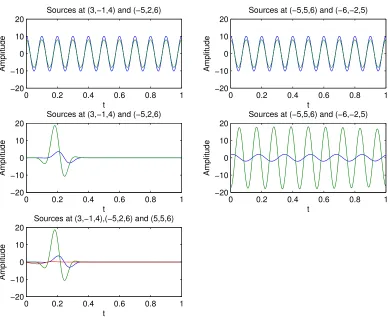
The pair sourcesmk(t), k= 1,2 for the first four scenarios and the treble sourcesmk(t), k=
1,2,3 for Scenario 5 are plotted respectively in Figure 1. By Scenarios 1 and 2, we com-pared the proposed procedure to the standard vector-beamformer (with c0 = 0) and to the other estimator-based beamformer, when there existed two highly correlated oscillatory sources (they have the same frequency and phase, but with slightly different amplitudes). By Scenarios 3 and 4, we tested these beamformers when there existed two unbalanced evoked response (or slightly dumped-oscillatory) sources. By Scenario 5, we assessed these beamformers when there were three spatially correlated source locations. In each scenario, with time-window width 1 and sample rate J, we sampled 30 data sets of Y(t) from the model
Y(t) =
p X
k=1
Hkmk(t) +ε(t), (5.5)
where in Scenarios 1∼4,mk(t),k= 1,2 are non-null time-courses at the two locations and
mk(t),3 ≤ k ≤ p are null time-courses at other grid points, while in Scenario 5, mk(t),
k = 1,2,3 are non-null time-courses at the three locations and mk(t),4 ≤ k ≤p are null
time-courses at other grid points. As before, {ε(t)} is a white noise process with noise level σ02. We considered various combinations of (n, p) = (91,2222) and (102,1487), and
J = 500,1000,2000, and 3000. Note that p is substantially larger than n and that the sources are sparse in the sense that there are only two or three non-null sources among p
candidates.
0 0.2 0.4 0.6 0.8 1 −20
−10 0 10 20
Amplitude
t
Sources at (3,−1,4) and (−5,2,6)
0 0.2 0.4 0.6 0.8 1
−20 −10 0 10 20
Amplitude
t
Sources at (−5,5,6) and (−6,−2,5)
0 0.2 0.4 0.6 0.8 1
−20 −10 0 10 20
Amplitude
t
Sources at (3,−1,4) and (−5,2,6)
0 0.2 0.4 0.6 0.8 1
−20 −10 0 10 20
Amplitude
t
Sources at (−5,5,6) and (−6,−2,5)
0 0.2 0.4 0.6 0.8 1
−20 −10 0 10 20
Amplitude
t
Sources at (3,−1,4),(−5,2,6) and (5,5,6)
Figure 1: The amplitude plots ofmk(t), k= 1,2 for Scenarios 1 to 4 and the amplitude plots
ofmk(t), k= 1,2,3 for Scenario 5. In these plots, the blue, green and red colored
curves are corresponding to the amplitudes ofmk(t), k= 1,2,3 respectively.
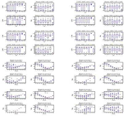
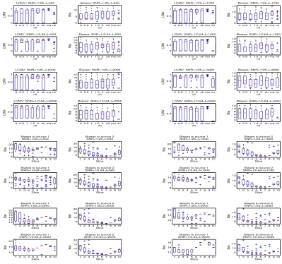
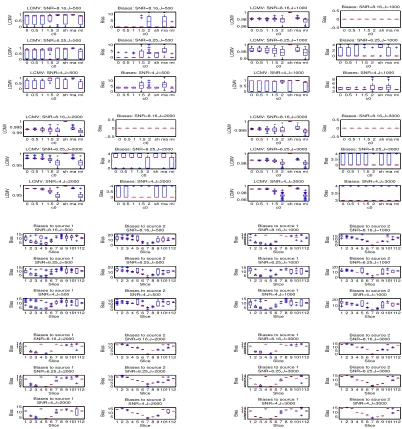
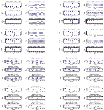
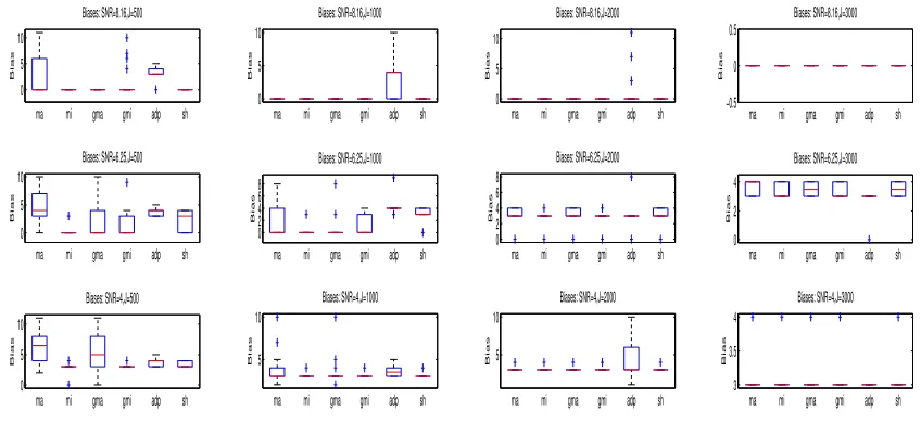
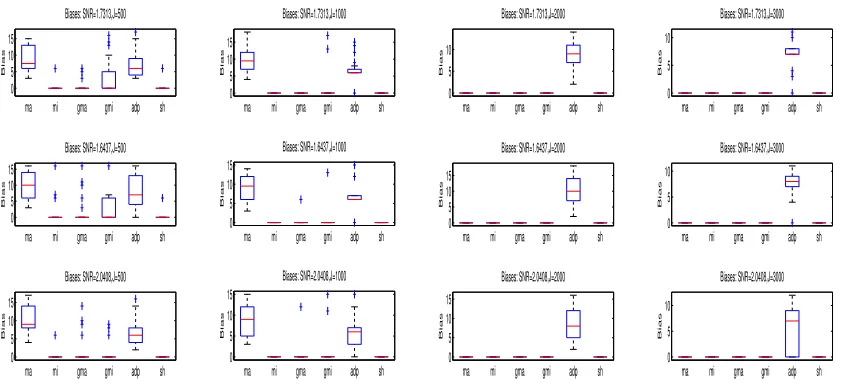
To compare the procedures ma, mi and sh with the procedures gma, gmi and adp based on the generalized and adaptive thresholding, we again generated 30 data sets from model (5.5) for each of the above four scenarios and for each combination of (n, p) = (91,2222) and (102,1487), andJ = 500,1000,2000,and 3000. We applied these procedures to each data set and calculated their localization biases respectively. As before, we displayed these biases by multiple box-whisker plots in Figures 6, 7 and 8. From these figures, we can see a dramatic improvement in localization performance of the hard thresholding-based procedure mi over the other procedures in Scenarios 1 and 2 and a slightly better or similar performance to ma, gma, gmi, adp and sh in Scenarios 3 and 4. This is striking because the existing studies have already shown that the soft (or generalized) and adaptive based covariance estimators can improve the hard thresholding-based covariance estimator in terms of estimation loss. The potential explanations for this phenomena are as follows: (1) The procedureadpmay lose efficiency by not using the pre-stimulus data. (2) The existing covariance estimators were aimed to improve the estimation accuracy by reducing the estimation loss (the distance between the estimator and the true covariance matrix) or by increasing the sensitivity and specificity in recovering sparse entries in the true covariance matrix (Rothman et al., 2009; Cai and Liu, 2011). Unfortunately, the sparsity in MEG means a sparse signal distribution, which is quite different from the entry sparsity of the sensor covariance matrix. Therefore, these estimators may be not efficient for improving the accuracy of the beamformer estimation which is related to the signal sparsity. In fact, our simulation experience suggests that besides the covariance estimation, there are other factors that can affect the performance of a beamformer such as the lead field matrix and the spatial distribution of signals in the brain. Therefore, the covariance estimator with a smaller estimation loss may not give rise to a beamformer with a lower localization bias.
To assess the performances of the six proceduresma,mi,gma,gmi,adpandshwhen there are more than two spatially correlated sources, we applied these procedures to the 30 data sets generated for Scenario 5. We calculated the average localization bias for each procedure and presented them in Figure 9. It can be seen from these plots that like in two-source scenarios, mi can have superior performance over the other procedures. However, compared the above result to those in Scenario 3, we can see that the source cancellation from r3 has increased the average localization bias from zero to the value of three.
Note that although Theorem 2 suggests that in general the localization bias will be reduced as the sampling rate increases, it does not implies the localization bias is a monotone function of the sampling rate (or the number of time instances). In fact, from row 4 in Figure 2 and row one in Figure 9, it can be seen that the localization bias whenJ = 500 is smaller than whenJ = 1000,2000 and 3000. A potential explanation is that in finite cases a higher sampling rate may cause a higher amount of leakage of background noises (in a neighborhood of the target location) into the neuronal activity index calculation.
5.2 Face-perception data
We applied the proposed methodology to human MEG data acquired in five sessions by Wakeman and Henson (Henson et al., 2011). In each session, 96 face trials and 50 scrambled face trials were performed on a healthy young adult subject. Each trial started with a central fixation cross (presented for a random duration of 400 to 600 ms), followed by a face or scrambled face (presented for a random duration of 800 to 1000 ms), and followed by a central circle for 1700 ms. The subject used either his/her left or right index finger to report whether he/she thought the stimulus was symmetrical or asymmetrical vertically through its center. The data were collected with a Neuromag VectorView system, containing a magnetometer and two orthogonal, planar gradiometers located at each of 102 positions within a hemispherical array situated in a light, magnetically shielded room. The sampling rate was 1100Hz. We focused our analysis on localizing non-null source positions, where neuronal activity increases for the face stimuli relative to the scrambled face stimuli.
For this purpose, we normalized the subject’s MRI scan to a MRI template by using the FieldTrip, on which a grid CTF system of 1 cm resolution was created with 1487 points. For each session, we applied the neuroimaging software SPM8 to read and preprocess the recorded data, and to epoch and average the data generated from the face stimulus trials and the scrambled face stimulus trials respectively. This gives rise to five 306×771 data matrices: the first 220 columns for 200ms pre-stimuli and the later 551 columns for the stimuli. For each session, we calculated the sample covariance ˆC and noise covariance ˆC0 by using the stimulus data and the pre-stimulus data respectively. We estimated the baseline noise level by ˆσ2
0, the minimum diagonal element in ˆC0. We applied the beamforming procedures ma, mi, gma, gmi, adp, and sh to the face data set and the scrambled face data set respectively, obtaining the log-contrasts at each grid point. Here, if there exist the negative eigenvalues of the covariance estimators (used inma,mi,gma,gmi,adp and sh), we set them to zeros and added 0 to them to make the resulting covariance estimators positive definite, where0 was determined by the maximum eigenvalue of the noise matrix ˆC0. For each procedure, we interpolated and overlaid its log-contrasts on the structural MRI of the subject, obtaining its index map. There were no visible differences among the maps derived fromma,mi,gma,gmi andsh. The map derived from theadp slightly differed from the rest. So, we reported only the mi-based and adp-based maps below.
(−4,3,8) cm, whereas theadp-based local peaks were located at (3,2,2)cm, (0,−1,11)cm, (−4,3,9)cm, (−6,−2,1)cm, (−4,−3,4)cm, (2,3,10)cm, (−4,−3,−1) cm, (−1,1,0) cm, (−3,6,3) cm, (−4,−4,5) cm, (−4,2,6) cm, (−5,3,7) cm, and (−4,3,8)cm. They are not the same as shown in Figure 11. Note that the previous simulations demonstrated that the procedure mi was expected to give a more accurate localization result than did the procedureadp.
Although the areas highlighted in Figures 10 and 11 were varying over sessions, they did reveal the following known regions of face perception: the occipital face area (OFA), the inferior occipital gyrus (IOG), and the superior temporal sulcus (STS), and the precuneus (PCu). Interestingly, in each session, we identified a pair of nearly symmetric sources, of which one was strongly powered while the other was weakly powered. This phenomenon occurred due to source cancellations that prevented the second source from identification as we have demonstrated in our simulation studies. The time-courses plots in Figure 12 showed the response differences under face stimuli and scrambled face stimuli during the time period 100ms∼300ms. The results are consistent with recent findings in face-perception studies by using an MEG-based multiple sparse prior approach (Friston et al., 2006; Henson et al., 2011) and by other empirical approaches (e.g., Pitcher et al., 2011; Kanwisher et al., 1997). However, in the first two papers, the authors made a parametric model assumption on source temporal correlation structures and imposed a limit on the number of candidate sources in the model, whereas in our approach, the model is non-parametric and allows for arbitrary number of candidate sources.
6. Discussion and Conclusion
In the present study, we have proposed a class of vector-beamformers by thresholding the sensor sample covariance matrix. The consistency and the convergence rate of the proposed vector-beamformer estimation have been proved in the presence of multiple sources. The theory has provided a basis for choosing the threshold τnJ =c0σ02
p
log(n)/J in the beam-former construction. However, it requires a number of conditions. As pointed out in Section 3, conditions (A1)∼(A4) are commonly used assumptions in literature for studying multiple time series (Sekihara and Nagarajan, 2008; Fan et al., 2011). We only need to validate the coherence stability condition which is new. Intuitively, the strength of correlations between sensors (therefore the absolute partial correlation) will increase when the number of sensors increases in general. Taking the face-perception data (session 1) as an example, we show how to validate it empirically by random sub-samples of the 306 sensors below. We take the first two peaks in Figure 8 as two true sources. They are located at CTF (-4,3,8) cm and (-4,-5,5) cm respectively. First, we reparametrize the lead field matrix as in Section 3. Then, for k= 1,2, ...,306,we randomly choose ksensors, obtaining a k×4461 sub lead field matrix for the 1487 voxels in the brain. We calculate the maximum absolute partial correlation d12(k) = max{d1|2, d2|2} between the two sources and the maximum absolute correlation dmax(k) = maxdx|2 for all voxels, where x is running over these voxels. Finally, we plot d12(k), dmax(k), and log(log(k)) against k = 1,2, ...,306 respectively as displayed in Figure 13. As expected, the result shows that both d12(k) and dmax(k) change very slowly when the number of sensors k changes, with a rate much slower than log(log(k)).
In real world situations, the underlying number of true sources,q needs to be estimated. The influence ofq on the beamformer estimators can be measured by the lead field partial correlation coefficient anq defined in Section 3. In this paper, local peaks on transverse
slices have been used to reduce the search space of sources. We can cluster the local peak values into two groups, one of which is taken as a group of potential sources. The size of the selected group gives an estimate of q. In the face-perception data, we have only presented the first two sources which are ranked higher than the remaining local peaks, because these two are of clear neurological implications. Our approach is non-parametric in the sense that we have not made any parametric assumptions on the model (1.1). However, if we are willing to assume a family of parametric models for background noises, then we can determineq via model selection criteria such as Bayesian information criterion.
By theoretical and empirical studies, we have shown that due to source cancellations, the beamformer power estimator can be inconsistent if the underlying multiple sources are not well separated in terms of a lead field distance. Unlike the existing theories in the literature, the new theory is applicable to more general scenarios, where multiple sources exist and the sensor covariance matrix are estimated from the data. In the new theory, we do assume that the powers of the unknown no-null sources as well as the underlying number
q are not growing with the number of sensorsn. This assumption is natural to neurologists and has simplified mathematical derivations of the theory very much. However, the theory can be extended to the case where these quantities are growing with n. In the theory, we have not impose any constraint onp as we only consider local behavior of beamformers. If we want to investigate global properties of the neuronal activity map, then some constraints need to be imposed on the growth rate of p with respect ton.
The performances of the proposed beamformers have further been assessed by simula-tions and real data analyses. We have demonstrated that thresholding the sensor covariance matrix can help reduce the source localization bias when the data have a low SNR value. We have applied the vector-beamformer to an MEG data set for identifying the active regions related to human face perception. Some excellent agreements have been found between the current results and the existing neurological facts on human face perception. Finally, we note that there are other ways to measure the contrast between two source covariances such as the information-divergence. The theory can be easily extended to this case. The details will be presented elsewhere.
7. Proofs
In this section we prove the theorems and corollaries in Section 3. To prove Theorem 1, we need the following lemma.
Lemma 10 If anq → ∞ as n→ ∞, then we have
HjTCk−1Hj = bjj|k+
cjj|k
n +O(a
−2
nk), bjj|k= Σj−1, for 1≤j≤k
HjT1Ck−1Hj2 =
cj1j2|k
n +O(a
−2
nk), for 1≤j16=j2 ≤k
HjTCk−1Hx = bjx|k+
cjx|k
n +O(a
−2
nk), for 1≤j ≤k, x /∈Rk
whereank =nmin1≤j≤k−1tr a(j+1)(j+1)|j
,Rk={r1, . . . , rk},Ck =Pjk=1HjTΣjHj+σ20In, andayx|k,byx|kandcjj|kare defined before and the otherc0sare defined iteratively as follows:
cj1j2|k=
bj1k|(k−1)Σ
−1
k a
−1
kk|(k−1), 1≤j1 ≤k−1, j2 =k
Σ−k1a−kk1|(k−1)bkj2|(k−1), 1≤j2 ≤k−1, j1 =k
cj1j2|(k−1)−bj1k|(k−1)a
−1
kk|(k−1)bkj2|(k−1), 1≤j1 6=j2≤k−1.
cjx|k =
akk|(k−1)Σk −1
bkx|(k−1) − I3+bkk|(k−1)
akk|(k−1)Σk −1
akx|(k−1)
o
, j=k
cjx|(k−1)−cjk|(k−1)a−kk1|(k−1)akx|(k−1)
−bjk|(k−1)a−kk1|(k−1)bkx|(k−1) 1≤j≤k−1 +bjk|(k−1)a−kk1|(k−1)
Σ−k1+bkk|(k−1)
a−kk1|(k−1)akx|(k−1).
Proof Note that under the stability condition and the assumption thatanq → ∞, we have
byx|k =O(1), 1≤k≤q. And for any rx in the source space,
c1x|1
n =O(n
−1), cyx|k
n =O(a
−1
n(k−1)),1≤y≤k,2≤k≤q. We prove the lemma by induction. Fork= 1, we have
C1−1 = σ0−2In−σ0−4H1(Σ−11+nσ −2
0 I3)−1H1T,
H1TC1−1H1 = nσ0−2I3−n2σ0−4(Σ−11+nσ0−2I3)−1 = nσ0−2 I3−
I3+ Σ−11
σ02 n
−1!
= nσ0−2 I3+nΣ1σ0−2
−1
= Σ−11 I3−σ20Σ−11/n
+O(n−2) = Σ−11−Σ−11σ02Σ−11/n+O(n−2) = b11|1+
c11|1
n +O(n
−2), where
b11|1= Σ−11, c11|1 =−σ02Σ −2 1 . Analogously,
H1TC1−1Hx = σ−2H1THx−σ0−4n(Σ −1 1 +nσ
−2 0 I3)
−1HT
1Hx
= I3− I3+ Σ−11σ02/n
−1
H1THx
=
I3+
n σ02Σ1
−1
H1THx
= Σ−11
I3+
σ02 nΣ
−1 1
−1
ρ1x
= Σ−11ρ1x−Σ−11σ02Σ −1
1 ρ1x/n+O(n−2)
= b1x|1+
c1x|1
n +O(n
where
b1x|1 = Σ−11ρ1x, c11|1 =−Σ−12σ20ρ1x.
And
HyTC1−1Hx = σ0−2HyTHx−σ−04HyTH1(Σ−11+nσ −2
0 I3)−1H1THx
= nσ0−2ρyx−σ0−4HyTH1
σ02
n I3+σ
2 0Σ−11/n
−1
H1THx
= nσ0−2ρyx−nσ0−2ρy1 I3−σ20Σ−11/n
ρ1x+O(n−1)
= nσ0−2ρy1x+ρy1Σ1−1ρ1x+O(n−1)
= nayx|1+byx|1+O(n−1), where
ρy1x=ρyx−ρy1ρ1x, ayx|1 =σ0−2ρy1x, byx|1=ρy1Σ−11ρ1x.
This implies the lemma holds for k= 1.
Assuming the lemma holds for the cases with less or equal to k sources, we show that it is also true for the case withk+ 1 sources by invoking the matrix inversion formulas
Ck−+11 = Ck−1−Ck−1Hk+1 Σ−k+11 +HkT+1C −1
k Hk+1
−1
HkT+1Ck−1, (7.6)
Ck−1 = Ck−+11 +Ck−+11 Hk+1Σk+1HkT+1Ck−1.
The details are as follows. For 1≤j≤k,
HjTCk−+11 Hj = HjTCk−1Hj− H T
j Ck−1Hk+1
× Σ−k+11 +HkT+1Ck−1Hk+1
−1
HkT+1Ck−1Hj
= bjj|k+
cjj|k
n +O(a
−2
nk)−
bj(k+1)|k+
cj(k+1)|k
n +O(a
−2
nk)
× Σ−k+11 +na(k+1)(k+1)|k+b(k+1)(k+1)|k+O(a−nk1) −1
×bj(k+1)|k+
cj(k+1)|k
n +O(a
−2
nk) T
= bjj|k+
cjj|k
n +O(a
−2
nk)
− bj(k+1)|k+O(a−nk1
(na(k+1)(k+1)|k)−1−O(a−n(2k+1))
× bj(k+1)|k+O(a−nk1) T
= bjj|k+
cjj|k
n −
1
nbj(k+1)|ka
−1
(k+1)(k+1)|kb T
j(k+1)|k+O(a
−2
n(k+1)) = bjj|(k+1)+
cjj|(k+1)
n +O(a
−2
n(k+1)). For j=k+ 1, we have
HjTCk−+11 Hj = HkT+1C −1
k+1Hk+1 =HkT+1C −1
k Hk+1 I3+ Σk+1HkT+1C −1
k Hk+1
−1
= na(k+1)(k+1)|k+b(k+1)(k+1)|k+O(a−nk1)
= na(k+1)(k+1)|k+b(k+1)(k+1)|k+O(a−nk1)
na(k+1)(k+1)|k −1
×I3+ (na(k+1)(k+1)|k)−1Σ−k+11 +O(a −2
n(k+1))
−1
Σ−k+11 = Σ−k+11 − 1
nΣ
−1
k+1a −1
(k+1)(k+1)|kΣ
−1
k+1+O(a
−2
n(k+1)) = b(k+1)(k+1)|(k+1)+
c(k+1)(k+1)|(k+1)
n +O(a
−2
n(k+1)). This completes the proof of the first equation in the lemma.
To prove the second equation in the lemma, we let
B =
Σk+1na(k+1)(k+1)|k −1
+
Σk+1na(k+1)(k+1)|k −12
×Σk+1b(k+1)(k+1)|k
Σk+1na(k+1)(k+1)|k −12
.
Then, when 1≤j1≤k,j2 =k+ 1, we have
HjT1Ck−+11 Hj2 = H T j1C
−1
k+1Hk+1=H
T j1C
−1
k Hk+1
I3+ Σk+1HkT+1Ck−1Hk+1
−1 =
bj1(k+1)|k+
1
ncj1(k+1)|k+O(a
−2
nk)
× I3+ Σk+1 na(k+1)(k+1)|k+b(k+1)(k+1)|k+O(a−nk1 −1
=
bj1(k+1)|k+
1
ncj1(k+1)|k+O(a
−2
nk)
Σk+1na(k+1)(k+1)|k −12
×(I3+B+O(an−(2k+1)))−1
Σk+1na(k+1)(k+1)|k −1
2
= bj1(k+1)|k
Σk+1na(k+1)(k+1)|k −12
× I3+O (na(k+1)(k+1)|k)−1 Σk+1na(k+1)(k+1)|k −1
2 +O(a−2 n(k+1)) = 1
nbj1(k+1)|kΣ
−1
k+1a −1
(k+1)(k+1)|k+O(a
−2
n(k+1)) = cj1(k+1)|(k+1)
n +O(a
−2
n(k+1)). Similarly, when 1≤j1 6=j2 ≤k, we have
HjT1Ck−+11 Hj2 = H T j1C
−1
k Hj2 −H
T j1C
−1
k Hk+1 Σ−k+11 +H
T
k+1Ck−1Hk+1
−1
HkT+1Ck−1Hj2
= 1
ncj1j2|k+O(a
−2
nk)−
1
nbj1(k+1|k)a
−1
(k+1)(k+1)|kb(k+1)j2|k+O(a
−2
n(k+1)) = 1
ncj1j2|(k+1)+O(a
−2
n(k+1)).
We complete the proof of the second equation in the lemma. To prove the third equation in the lemma, we let
D = na(k+1)(k+1)|kΣk+1
−1
+ na(k+1)(k+1)|kΣk+1
−12
×b(k+1)(k+1|k)Σk+1 na(k+1)(k+1)|kΣk+1
−12
,
F = (na(k+1)(k+1)|k)− 1
2 Σ−1
k+1+b(k+1)(k+1)|k
Then, forj =k+ 1,
HjTCk−+11 Hx =
I3+HkT+1Ck−1Hk+1Σk+1 −1
HkT+1Ck−1Hx
=
I3+na(k+1)(k+1)|kΣk+1+b(k+1)(k+1)|kΣk+1+O(a−nk1)
−1
×
na(k+1)x|k+b(k+1)x|k+O(a−nk1)
= na(k+1)(k+1)|kΣk+1
−12
(I3+D+O(a−n(2k+1)))−1 na(k+1)(k+1)|kΣk+1
−12
×
na(k+1)x|k+b(k+1)x|k+O(a−nk1)
= a(k+1)(k+1)|kΣk+1
−1 2
n
I3−D+O(a−n(2k+1))
o
× a(k+1)(k+1)|kΣk+1
−12
a(k+1)x|k+b(k+1)x|k/n+O(a−nk1)/n
= a(k+1)(k+1)|kΣk+1
−1
a(k+1)x|k
− a(k+1)(k+1)|kΣk+1
−1/2
D a(k+1)(k+1)|kΣk+1
−1/2
a(k+1)x|k
+O(a−n(3k+1)) + 1
n a(k+1)(k+1)|kΣk+1
−1
b(k+1)x|k+O(a−n(2k+1))
= a(k+1)(k+1)|kΣk+1
−1
a(k+1)x|k+
1
n a(k+1)(k+1)|kΣk+1
−1
×nb(k+1)x|k− I3+b(k+1)(k+1)|kΣk+1
a(k+1)(k+1)|kΣk+1
−1
a(k+1)x|k o
+O(a−n(2k+1)) = b(k+1)x|(k+1)+
1
nc(k+1)x|(k+1)+O(a
−2
n(k+1)). For 1≤j ≤k, we have
HjTCk−+11 Hx = HjTC
−1
k Hx−H
T
j C
−1
k Hk+1 Σ−k+11 +H
T k+1C
−1
k Hk+1
−1
HkT+1Ck−1Hx
= bjx|k+
1
ncjx|k+O(a
−2
nk)−
bj(k+1)|k+
1
ncj(k+1)|k+O(a
−2
nk)
× Σ−k+11 +na(k+1)(k+1)|k+b(k+1)(k+1)|k+O(a−nk2) −1
× na(k+1)x|k+b(k+1)x|k+O(a−nk1)
= bjx|k+
1
ncjx|k+O(a
−2
nk)−
bj(k+1)|k+
1
ncj(k+1)|k+O(a
−2
nk)
×(na(k+1)(k+1)|k)−1/2
I3+F +O(a−nk2)
−1
(na(k+1)(k+1)|k)−1/2
× na(k+1)x|k+b(k+1)x|k+O(a−nk1)
= bjx|k+
1
ncjx|k+O(a
−2
nk)−
bj(k+1)|k+
1
ncj(k+1)|k+O(a
−2
nk)
×a−(k1+1)(k+1)|ka(k+1)x|k−a
−1/2
(k+1)(k+1)|kF a
−1/2
(k+1)(k+1)|ka(k+1)x|k+O(a
−2
nk)
(na(k+1)(k+1)|k)−1b(k+1)x|k−a
−1/2
(k+1)(k+1)|kF a
−1/2
(k+1)(k+1)|kb(k+1)x|k/n
+O(a−n(2k+1))
= bjx|k+
1
ncjx|k+O(a
−2
nk)−
bj(k+1)|k+
1
ncj(k+1)|k+O(a
−2
nk)
×
a−(k1+1)(k+1)|ka(k+1)x|k−
1
na
−1
(k+1)(k+1)|k(Σ
−1
k+1+b(k+1)(k+1)|k)
×a−(k1+1)(k+1)|ka(k+1)x|k
1
na
−1
(k+1)(k+1)|kb(k+1)x|k+O(a−n(2k+1))
= bjx|k+
1
ncjx|k−bj(k+1)|ka
−1
(k+1)(k+1)|ka(k+1)x|k
−1
n
n
cj(k+1)|ka−(k1+1)(k+1)|ka(k+1)x|k+bj(k+1)|ka−(k1+1)(k+1)|kb(k+1)x|k
−bj(k+1)|ka(−k1+1)(k+1)|k
Σ−k+11 +b(k+1)(k+1)|k
a−(k1+1)(k+1)|ka(k+1)x|k o
+O(a−n(2k+1))
= bjx|k−bj(k+1)|ka−(k1+1)(k+1)|ka(k+1)x|k+
1
ncjx|(k+1)+O(a
−2
n(k+1)). (7.7) Note that fork=j,
ajx|j =ajx|(j−1)−ajj|(j−1)a−jj1|(j−1)ajx|(j−1)= 0.
Assuming that for k = j+m, m > 0, the statement is true, i.e., ajx|(k+m) = 0 for all x. Then,
ajx|(j+m+1) = ajx|(j+m)−aj(j+m+1)|(j+m)a−(j1+m+1)(j+m+1)|(j+m)a(j+m+1)x|(j+m) = 0.
By induction, we have thatajx|k = 0 for allx,j≤k. This implies that and
bjx|(k+1) = bjx|k−bj(k+1)|ka−(k1+1)(k+1)|ka(k+1)x|k
by the definition ofbjx|(k+1).Combining this with (7.7), we complete the proof of the third equation in the lemma.
Finally, we turn to the last equation in the lemma. Assume that the equation holds for the case k. We show that it also holds for k+ 1 below. Forx, y /∈Rk+1 (thus x, y /∈Rk),
by the assumption, we have
HyTCk−1Hx=nayx|k+byx|k+O(a−nk1).
This together with (7.6) yields
HyTCk−+11 Hx = HyTCk−1Hx−HyTCk−1Hk+1 Σ−k+11 +H
T
k+1Ck−1Hk+1
−1
HkT+1Ck−1Hx
= nayx|k+byx|k+O(a−nk1)− nay(k+1)|k+by(k+1)|k+O(a−nk1)
× Σ−k+11 +na(k+1)(k+1)|k+b(k+1)(k+1)|k+O(a−nk1) −1
× na(k+1)x|k+b(k+1)x|k+O(a−nk1)
×
(na(k+1)(k+1)|k)−1−
1
n2a −1
(k+1)(k+1)|k Σ
−1
k+1+b(k+1)(k+1)|k
×a−(k1+1)(k+1)|k+O(a−n(3k+1)) nay(k+1)|k+by(k+1)|k+O(a−nk1)
= nayx|k+byx|k+O(a−nk1)− n
ay(k+1)|ka(−k1+1)(k+1)|k
−ay(k+1)|ka(−k1+1)(k+1)|k Σ
−1
k+1+b(k+1)(k+1)|k
a−(k1+1)(k+1)|k/n
+by(k+1)|ka(−k1+1)(k+1)|k/n+O(a
−2
n(k+1))
o
× na(k+1)x|k+b(k+1)x|k+O(a−nk1)
= n
h
ayx|k−ay(k+1)|ka−(k1+1)(k+1)|ka(k+1)x|k i
+hbyx|k−by(k+1)|ka−(k1+1)(k+1)|ka(k+1)x|k−ay(k+1)|ka(−k1+1)(k+1)|kb(k+1)x|k
+ay(k+1)|ka(−k1+1)(k+1)|k Σ
−1
k+1+b(k+1)(k+1)|k
a−(k1+1)(k+1)|ka(k+1)x|k i
+O(a−n(1k+1))
= nayx|(k+1)+byx|(k+1)+O(a−n(1k+1)). The proof is completed.
Proof of Theorem 1. Note thatbyx|1 =ρ(ry, r1)Σ−11ρ(x1, x),ayx|1=σ0−2(ρyx−ρy1ρ1x),
and both are bounded. By induction and the stability condition, it can be shown thatayx|k
and byx|k are bounded for 2 ≤ k ≤ q. If anq is bounded, then there exists km such that
na(km+1)(km+1)|km = O(1) and ankm = min1≤j≤km−1na(j+1)(j+1)|j → ∞ as n tends to
infinity. By Lemma 10, we have
HkTm+1Ck−1
mHkm+1 = na(km+1)(km+1)|km+b(km+1)(km+1)|km+O(a
−1
nkm),
which is bounded and non-negative definite. Furthermore, there exists an orthogonal matrix
Qand a diagonal matrix D= diag(d1, d2, d3) such that Σ1k/2
m+1H
T km+1C
−1
kmHkm+1Σ
1/2
km+1=QDQ
T.
Therefore,
HkTm+1Ck−1
m+1Hkm+1
=HkTm+1Ck−1
mHkm+1
I3− Σ−km1+1+HkTm+1C
−1
kmHkm+1
−1
HkTm+1Ck−1
mHkm+1
=HkTm+1Ck−1
mHkm+1 Σ
−1
km+1+H
T km+1C
−1
kmHkm+1
−1
Σ−k1
m+1
=HkTm+1Ck−1
mHkm+1Σ
1/2
km+1
I3+ Σ1k/m2+1HkTm+1C
−1
kmHkm+1Σ
1/2
km+1
−1
Σ−k1/2
m+1
= Σ−k1/2
m+1QDQ
T I
3+QDQT
−1
Σ−k1/2
m+1
= Σ−k1/2
m+1 I3+QD
−1QT−1
Σ−k1/2
m+1
= Σ−k1/2
m+1 Q(I3+D
−1)QT−1
Σ−k1/2
m+1
= Σ−k1/2
m+1Q(I3+D
−1)−1QTΣ−1/2
Note that Σ1k/m2+1HkTm+1Ck−m1Hkm+1Σ
1/2
km+1=O(1), which implies thatdk ≥0,1≤k≤3 are
bounded. We can find a positive constant 0 such that max1≤k≤3(1 +dk−1)−1 <(1 +0)−1 when nis large enough. Consequently, for any vector a∈R3 with||a||= 1, we have
aTΣ1k/2
m+1Q(I3+D
−1)QTΣ1/2
km+1a >(1 +0)a
TΣ1/2
km+1QQ
TΣ1/2
km+1a,
which shows that Σ1k/2
m+1Q(I3+D
−1)QTΣ1/2
km+1 (thus
HkT
m+1C
−1
km+1Hkm+1
−1
due to (7.8)) is asymptotically larger than Σkm+1(1 +0).
We now consider the case where anq → ∞. Forj=q, by Lemma 10, we have
cqq|q
n = −Σ
−1
q
naqq|(q−1)
−1
Σ−l 1 =O(a−nq1),
HqTCq−1Hq −1
=
h
Σ−q1+cqq|q
n +O(a
−2
nq) i−1
,
= Σ1q/2
h
I3+ Σ1q/2
cqq|q
n Σ
1/2
q +O(a
−2
nq) i−1
Σ1q/2 = Σ1q/2
h
I3−Σ1q/2
cqq|q
n Σ
1/2
q +O(a
−2
nq) i
Σ1q/2 = Σq−
naqq|(q−1)
−1
+O(a−nq2) asn→ ∞.For 1≤j≤q−1, by Lemma 10, we have
HjTCq−1Hj = Σ−j1+
cjj|q
n +O(a
−2
nq),
where cjj|q
n =O(a
−1
nq). This entails
HjTCq−1Hj −1
= Σ1j/2
I3+ 1
nΣ
1/2
j cjj|qΣ
1/2
j +O(a
−2
nq) −1
Σ1j/2 = Σ1j/2
I3− 1
nΣ
1/2
j cjj|qΣ
1/2
j +O(a
−2
nq)
Σ1j/2 = Σj −
1
nΣjcjj|qΣj+O(a
−2
nq).
For any location rx, by Lemma 10, we have
HxTCq−1Hx −1
= 1
n
I3+ 1
na
−1
xx|qbxx|q+O(a−nq2) −1
a−xx1|q
= 1
n
I3− 1
na
−1
xx|qbxx|q+O(a
−2
nq)
a−xx1|q
= 1
na
−1
xx|q−
1
n2a −1
xx|qbxx|qa
−1
xx|q+O(a
−3
nq).
The proof is completed.
Proof of Corollary 2. First, let An =
Hkm+1
TC−1
l Hkm+1
−1
. If anq = O(1) and