A Fast High Order Algorithm for 3D Helmholtz Equation with Dirichlet Boundary

(1)

http://www.sciencepublishinggroup.com/j/acm doi: 10.11648/j.acm.20180704.11

ISSN: 2328-5605 (Print); ISSN: 2328-5613 (Online)

A Fast High Order Algorithm for 3D Helmholtz Equation

with Dirichlet Boundary

Sheng An

*

, Gendai Gu, Meiling Zhao

School of Mathematics and Physics, North China Electric Power University, Baoding, China

Email address:

*

Corresponding author

To cite this article:

Sheng An, Gendai Gu, Meiling Zhao. A Fast High Order Algorithm for 3D Helmholtz Equation with Dirichlet Boundary. Applied and Computational Mathematics. Vol. 7, No. 4, 2018, pp. 180-187. doi: 10.11648/j.acm.20180704.11

Received: July 26, 2018; Accepted: August 13, 2018; Published: September 11, 2018

Abstract:

Helmholtz equation is widely applied in the scientific and engineering problem. For the solution of the three-dimensional Helmholtz equation, the computational efficiency of the algorithm is especially important. In this paper, in order to solve the contradiction between accuracy and efficiency, a fast high order finite difference method is proposed for solving the three-dimensional Helmholtz equation. First, a traditional fourth order method is constructed. Then, fast Fourier transformation are introduced to generate a block-tridiagonal structure which can easily divide the original problem into small and independent subsystems. For large 3D problems, the computation of traditional discrete Fourier transformation is less efficient, and the memory requirements increase rapidly. To fix this problem, the transformed coefficient matrix is constructed as a sparse structure. In light of the sparsity, the algorithm presented in this paper requires less memory space and computational cost. This sparse structure also leads to independent solving procedure of any plane in the domain. Therefore, parallel method can be used to solve the Helmholtz equation with large grid number. In the end, three numerical experiments are presented to verify the effectiveness of the fast fourth-order algorithm, and the acceleration effect to use the parallel method has been demonstrated.

Keywords:

Helmholtz Equation, Fourier Transformation, Parallel Implementation

1. Introduction

In this paper, we consider the following Helmholtz equation

∆ , , , , , , , in Ω, # (1) with Dirichlet boundary condition

, , , , , on Ω, # (2) where is the wave number. Helmholtz equation is widely applied to wave propagation and acoustic scattering problem, viscous and heat transfer problems and electromagnetic scattering problems.

In recent years, there has been tremendous interest in developing algorithms for solving the Helmholtz equation. The precise numerical solution of Helmholtz equation is of great importance. Most algorithms were initially developed for the two-dimensional case, such as finite element method,

(2)

Helmholtz equation. Sutmann combined different high order finite difference schemes and proposed a more efficient algorithm in [14, 15]. Furthermore, Gordon et al. extend the sixth-order finite difference method to high and variable wave number with CARP-CG algorithm in [16, 17]. Due to the heavy computational cost the efficiency of the algorithm for solving three-dimensional Helmholtz equation is especially important. The Fourier method has many advantages for solving the Helmholtz equation. Together with the symmetry of the high-order finite difference operator, the Dirichlet problems can be solved easily with sine transformation.

In this paper, our aim is to discretize the Helmholtz equation with fourth-order finite difference method and build a fast algorithm using the discrete Fourier-sine transformation. On the other hand, the traditional Fourier transformation in three dimensions needs considerable memory requirement especially for large wave number equations. In views of this problem, twice Fourier transformation are applied for the discrete Helmholtz equation.

The paper is organized as follows. In Section 2, a fourth-order finite difference method was proposed to discrete the three-dimensional Helmholtz equation. In Sections 3 and 4, a fast high algorithm is developed for solving the three-dimensional Helmholtz equation. Section 5 describes the parallel implementation for the three-dimensional Helmholtz equation. Moreover, three numerical examples prove the validity and feasibility of the proposed method. The paper is concluded in Section 6.

2. The Fourth-Order Finite Difference

Method

We consider a fourth-order finite difference method of (1), whereΩ is the model domain and Ω is the boundary of the domain. , , is an given continuous function. In this paper, a cubic domain Ω 0, 0, 0, is considered as the solution field. Firstly, the uniform partition is define as , , !#$%,&$%,'$%_{, ,"} in Ω. Without loss of generality, we consider the case of ( ∆ ∆ ∆ since it can be extended to the general situation. For any point

, , in Ω the standard second order central difference operator can be written as

)* , , $%, , + 2₍, , -%, , ,

). , , , $%, + 2₍, , , -%, ,

)/ , , , , $%+ 2₍, , , , -%,

where _{, ,}, 0 1, 2, … , 3, 4 1, 2, … , 5, 6 1, 2, … , 7 refers to the fourth-order finite difference solution of the three-dimensional Helmholtz equation. refers to the fourth-order finite difference solution of the three-dimensional Helmholtz equation.

The fourth-order finite difference form can be obtained in the interior of Ω.

81 9:_%;:< =)* ). )/> , , ; :

? =)*). )*)/ ).)/> , , , , ;:

% =)*). )*)/ ).)/> , , @ (A .

# (3)

Figure 1 depicts the contributions to the 19-points stencil in an given axes, where C_% 1 9:_%;:, C ;_?:.

(3)

Moreover, (3) can be written in the matrix form

81 9_%:;:< D#E F&E F' F#E D&E F' F#E F&E D' G ;:

? D#E D&E F' F#E D&E D' D#E F&E D' G G GH

I ;_%: D#E F&E F' F#E D&E F' F#E F&E D' I IH,

# (4)

where

D# _{( tridiag 1, +2,1 , D}1 & _{( tridiag 1, +2,1 , D}1 ' _{( tridiag 1, +2,1 ,}1

G = %,%,%, O , %,%,', %, ,%, O , %, ,', O , %,&,', O , #,&,'>P,

I =%,%,%, O , %,%,', %, ,%, O , %, ,', O , %,&,', O , #,&,'>P, and the symbol Q represents the Kronecker product. F_#, F_&, F_' and F_#&' are identity matrices, and the subscripts denote their dimension. D_#, D_& and D_' are 3 3, 5 5 and 7 7 tridiagonal matrices respectively. G_H and I_H contain boundary values subtracted from G and I.

3. The Explanation of the Boundary

Parts

The boundary part G_H consists 18 parts which are related to six surfaces and twelve edges of the domain, they are R_HSTU, R_HVTSSTW, R_{H XYS}, R_{HZ [;S}, R_HYZT\S, R_HV]^9,

__HS%, __HS , __HS`, __HSA, __H^%, __H^ , __H^`, __H^A, __HV%, __HV , __HV`, __HVAIn this section, only the detailed discussion of

RH XYS and __HS% will be given, the other items can be deduced in similar way.

For a point _%, , in the domain, points on the left surface of the domain = , , >, = , , _$%> ,

= , , -%>, = , -%, >, = , $%, > will generate the boundary part R_{H XYS} as shown in Figure 2.

Figure 2. The corresponding points of R_{H XYS}.

R_{H XYS} can be written as follows

R_{H XYS} =C #aE D&E F' C #aE F&E D'>G,:,:

=C% #aE F&E F'>G,:,:

# (5)

where _#_a _;%_: 1,0, … ,0 _#P.

Analogously, __HS% is related to three points

= $%, , >, = -%, , >, = , , $%>. Therefore, we have

_Hca C F#Q &%Q ' G:, ,'$%. # (6)

where _&% _;%_: 1,0, … ,0 _&P, _' _;%_: 0,0, … ,1 _'P.

Moreover, the boundary part dI includes six parts. I_H can be written as follows

IH IHSTU IHVTSSTW IH XYS IHZ [;S IHefghc

I_HV]^9# (7)

where

I_HSTU C% F#E F&E ' I:,:,'$%,

I_HVTSSTW C% F#E F&E '% I:,:, ,

I_{H XYS} C% #%E F&E F' I,:,:,

IHZ [;S C% # E F&E F' I#$%,:,:,

IHefghc C% F#E &%E F' I:, ,:,

IHV]^9 C% F#E & E F' I:, ,:

'% _{( 1,0, … ,0}1 'P, # _{( 0,0, … ,1}1 #P,

& _{( 0,0, … ,1}1 &P.

4. The Fast Algorithm for 3D Helmholtz

Equation

For the tridiagonal Toeplitz matrix D_# and D_&, we have

R#D#R# Λ% diag j%, j , … , j# ,

R&D&R& Λ diag k%, k , … , k& , where

R# , l_#$%8sin_#$%n< ,

j +A #$%_] :sin _#$%n , 1 o 0, 4 o 3, ##

(4)

R# and R_& are discrete Fourier-sine transformation matrices. R_& and k_S, p = 1,2, … , 5 can be defined similarly as

(8). Multiplying R_#⊗ R_&⊗ F_' on both side of (4), the following formula can be obtained

81 +9:_%;:< Λ%⊗ F&⊗ F'+ F#⊗ Λ ⊗ F'+ F#⊗ F&⊗ D' Gq

+;_?: Λ%⊗ Λ ⊗ F'+ F#⊗ Λ ⊗ D'+ Λ%⊗ F&⊗ D' Gq + Gq + GqH

= Ir +;_%: Λ%⊗ F&⊗ F'+ F#⊗ Λ ⊗ F'+ F#⊗ F&⊗ D' Ir + IrH,

# (9)

where Gq = R_#⊗ R_&⊗ F_' G, Ir = R_#⊗ R_&⊗ F_' I, Gq_H= R_#⊗ R_&⊗ F_' G_H, Ir_H= R_#⊗ R_&⊗ F_' I_H. Multiplying R_#⊗ R_&⊗ F_' on each part of Gq_H, there follows

Rs_HSTU= C Λ%⊗ F&⊗ ' + C F#⊗ Λ ⊗ ' + C% F#⊗ F&⊗ ' Gq:,:,'$%,

Rs_HVTSSTW= C Λ%⊗ F&⊗ '% + C F#⊗ Λ ⊗ '% + C% F#⊗ F&⊗ '% Gq:,:, ,

RsHYZT\S = C Λ%⊗ R&⊗ F' + C F#⊗ R&⊗ D' + C% F#⊗ R&⊗ F' Gq:, ,:,

RsHV]^9 = C Λ%⊗ R&⊗ F' + C F#⊗ R&⊗ D' + C% F#⊗ R&⊗ F' Gq:,&$%,:,

Rs_{H XYS}= C R#⊗ t ⊗ F' Gq,:,:+ C R#⊗ F&⊗ F' Gqq ,:,:+ C% R#⊗ F&⊗ F' Gq,:,:

RsHZ [;S= C R#⊗ t ⊗ F' Gq#,:,:+ C R#⊗ F&⊗ F' Gqq#,:,:+ C% R#⊗ F&⊗ F' Gq#,:,:,

_rH %= C R#⊗ R&⊗ F' Gq, ,:, _rH = C R#⊗ R&⊗ F' Gq#$%, ,:,

_r_{H `}= C R#⊗ R&⊗ F' Gq#$%,&$%,:, _rH A= C R#⊗ R&⊗ F' Gq,&$%,:,

_r_HS%= C F#⊗ R&⊗ ' Gq:, ,'$%, _rHS = C F#⊗ R&⊗ '% Gq#$%, ,'$%,

_r_HS`= C R#⊗ F&⊗ ' Gq:,&$%,'$%, _rHS`= C R#⊗ F&⊗ ' Gq:, ,'$%,

_r_Hu% = C R#⊗ F&⊗ '% Gq:, , , _rHu = C R#⊗ F&⊗ '% Gq#$%,:, ,

_r_H^`= C F#⊗ R&⊗ '% Gq:, &$%, , _rH^A= C F#⊗ R&⊗ '% Gq,:, ,

where

Gq ,:,:= #%⊗ R&⊗ F' G ,:,:, Gqq,:,:= #%⊗ R&⊗ D' G ,:,:,

Gq#,:,:= # ⊗ R&⊗ F' G#,:,:, Gqq#,:,:= # ⊗ R&⊗ D' G#,:,:. Multiplying R_#⊗ R_&⊗ F_& on Equation (6), there holds

Ir_HSTU = C% F#⊗ F&⊗ ' Ir:,:,'$%, IrHVTSSTW= C% F#⊗ F&⊗ '% Ir:,:, ,

Ir_{H XYS} = C% #%⊗ F&⊗ F' Ir,:,:, IrHZ [;S= C% # ⊗ F&⊗ F' Ir#$%,:,:,

IrHYZT\S = C% F#⊗ &%⊗ F' Ir:, ,:, IrHV]^9= C% F#⊗ & ⊗ F' Ir:, ,:,

Equation 9 is transformed into block-tridiagonal system, therefore, we can transform the original problem into the following equations

w81 +9:_%;:< =j F'+ k F'+ D'> +;

:

?=j k F'+ k D'+ j D'> + F'x Gq, ,:+ GqH , ,:

= Ir, ,:+ IrH , ,:, 0 = 1,2, … , 3; 4 = 1,2, … , 5. #

(10)

5. Numerical Experiments

5.1. Preparation for the Numerical Experiments

In this section, the algorithm is applied for three numerical experiments. And the performance of the algorithm is described using MATLAB on an eight processor computer.

One error measurement is used to weigh the difference between ∗_{, ,9} and _{, ,9}, where ∗_{, ,9} denotes the real solution of the three-dimensional Helmholtz equation.

(5)

{||}| ~_{357 € •}•` z, ,9+ , ,9• #,&,'

, , "%

‚

%

For different kinds of meshes, the convergence order can be written as

}|ƒ{| 6}„ _{{||}| … 1 .}{||}| …

5.2. Parallel Implementation

After deriving Gq by (10), the solution G of the three-dimensional Helmholtz equation is calculated by G

R#E R&E F' Gq. Due to the special form of the coefficient matrix, the computational procedure is independent for each

, 6 0,1, … , 7. Therefore, the fast algorithm proposed in Section 3 is well adapted for the parallel computation. The implementation under … processors is shown in Figure 3.

Figure 3. Partition of the three-dimensional mesh among … processors.

Example 1. Consider the problem

, , †‡ˆ n. †‡ˆ n/_{†‡ˆ=√ n>}

· w2 sinh=√2Œ > sinh 8√2Œ 1 + <x ,# (11)

with Dirichlet boundary conditions, where Ω 0,1

0,1 0,1 is a unit cubic.

• , ,, , 2 sin Œ sin Œ ,sin Œ sin Œ , 0 ,1, 0, , Ž •0,1•,

The numerical results for solving Gq and G are displayed in Table 1. Here CPU_”q and CPU_” denotes the computational time (s) for solving Gq and G respectively. After deriving Gq, we need to multiply R_#E R_&E F_' on the left side of Gq to compute the numerical solution of the Helmholtz equation. As we can see from Table 1, CPU_”q time is notably less than

CPU” time especially for large gird points. Moreover, the comparison of the computational time of three times Fourier transformation and twice Fourier transformation are given in Table 1. Here R_#E R_&E R_' and R_#E R_&E F_' represent two different transform operators.

Table 1. CPU time (s) and error for solving Gq and G.

• _š›œ–•E –—E –˜ –•E –—E ™˜

•q time (s) š›œ_• time (s) š›œ_•q time (s) š›œ_• time (s)

8 0.0381 0.0449 0.0499 0.2240

16 0.0634 0.8158 0.1947 0.2717

32 0.4535 28.6402 0.7144 0.4436

64 1.5009 1052.0414 3.2476 3.1560

128 9.0472 46725.2783 14.0811 60.283293

If the practical problem only needs some of the solutions of the Helmholtz equation, the algorithm can provide more precious numerical solutions on one of the surfaces. The

numerical solution on the face % with 1024 1024

(6)

Figure 4. The numerical solution on the face % with 3 1024.

∆ , 5, in Ω,

with boundary conditions corresponding to the exact solution

sin Œ sin Œ sin Œ . # (12) Figure 5 illustrates the numerical solution of (12) with

512 512 512 meshes.

Figure 5. The numerical solution of Equation (12) with 3 512.

The behavior of the parallel implementation was examined in Example 2. The results are displayed in Table 2. The results again verify the efficiency of the parallel processor. Moreover, we test the convergence order of the proposed fast high algorithm. The last column of Table 2 demonstrates the fourth-order convergence of the proposed algorithm. The line in Figure 6 is fitted by log error and log 3 and its slope is 4.0545.

Figure 6. log-log picture of 6}„ {||}| and 6}„ 3 and the slope of the fitted line is 4.0545.

-8 -7.5 -7 -6.5 -6 -5.5 -5 -4.5 -4 -3.5 -3

log(h)

-35 -30 -25 -20 -15 -10

lo

g

(E

rr

o

(7)

Table 2. CPU time (s) and error for solving Gq and G.

• š›œ_•q time (s) š›œ• time (s) error order

1 core 8 cores

8 0.0313 0.0162 0.2392 1.0145e-04

16 0.1008 0.1902 0.3019 5.6505e-06 4.1662

32 0.6519 3.2303 0.4358 3.3522e-07 4.0752

64 2.8458 56.5750 3.1811 2.0439e-08 4.0357

128 12.4757 1020.6792 50.2228 1.2621e-09 4.0174

256 56.7871 12472.1685 909.4857 7.8732e-11 4.0027

∆ 0, in Ω,

with boundary conditions corresponding to the exact solution

, , cos 2 cos=√1 >†‡ˆ¦ √§/ _{†‡ˆ¦ √§n}. # (13)

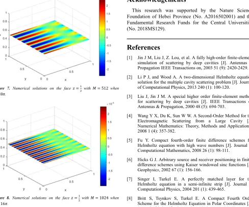
The figures of the numerical solutions G with different wave number in Figure 7 and Figure 8. As shown in Figures 7-8, the solutions of the Helmholtz equation is highly oscillating for large wave number.

Figure 7. Numerical solutions on the face % with 3 512 when

8Œ.

Figure 8. Numerical solutions on the face % with 3 1024 when

16Œ.

6. Conclusion

In this paper, we proposed an fourth-order fast algorithm for solving the three-dimensional Helmholtz equation. By multiplying the Fourier transform operator, the large system becomes some small independent systems. Moreover, in view of the special format of the coefficient matrix, we utilize the parallel processors to solve the equation. This implementation is especially efficient for solving the numerical solutions on one of the surfaces. Three numerical experiments have demonstrated the validity of the fourth-order fast algorithm.

Acknowledgements

This research was supported by the Nature Science Foundation of Hebei Province (No. A2016502001) and the Fundamental Research Funds for the Central Universities (No. 2018MS129).

References

[1] Jin J M, Liu J, Z. Lou, et al. A fully high-order finite-element simulation of scattering by deep cavities [J]. Antennas & Propagation IEEE Transactions on, 2003 51 (9): 2420-2429. [2] Li P J, and Wood A. A two-dimensional Helmholtz equation

solution for the multiple cavity scattering problem [J]. Journal of Computational Physics, 2013 240 (1): 100-120.

[3] Liu J, Jin J M. A special higher order finite-element method for scattering by deep cavities [J]. IEEE Transactions on Antennas & Propagation, 2000 48 (5): 694-703.

[4] Wang Y X, Du K, Sun W W. A Second-Order Method for the Electromagnetic Scattering from a Large Cavity [J]. Numerical Mathematics: Theory, Methods and Applications,. 2008 1 (4): 357-382.

[5] Fu Y. Compact fourth-order finite difference schemes for Helmholtz equation with high wave numbers [J]. Journal of Computational Mathematics, 2008 26 (1): 98-111.

[6] Hicks G J. Arbitrary source and receiver positioning in finite-difference schemes using Kaiser windowed sinc functions [J]. Geophysics, 2002 67 (1): 156-166.

[7] Singer I, Turkel E. A perfectly matched layer for the Helmholtz equation in a semi-infinite strip [J]. Journal of Computational Physics, 2004 201 (1): 439-465.

(8)

[9] Nabavi M, Siddiqui M. H. K, Dargahi J. A new 9-point sixth-order accurate compact finite-difference method for the Helmholtz equation [J]. Journal of Sound & Vibration, 2007 307(3): 972-982.

[10] Feng X F, Li Z L, Qiao Z H. High order compact finite difference schemes for the Helmholtz equation with discontinuous coefficients [J]. Journal of Computational Mathematics, 2011, 29 (3):324-340.

[11] Singer I, Turkel E. Sixth-order accurate finite difference schemes for the Helmholtz equation [J]. Journal of Computational Acoustics, 2006 14 (3): 339-351.

[12] Sutmann G. Compact finite difference schemes of sixth order for the Helmholtz equation [J]. Journal of Computational & Applied Mathematics, 2007 203 (1): 15-31.

[13] Sutmann G. Compact finite difference schemes of sixth order for the Helmholtz equation [J]. Journal of Computational & Applied Mathematics, 2007 203 (1): 15-31.

[14] Gordan D, Gordon R. Parallel solution of high frequency Helmholtz equations using high order finite difference schemes [J]. Applied Mathematics & Computation, 2012 218 (21): 10737-10754.

[15] Helmholtz solver by domain decomposition and modified Fourier method [J]. Siam Journal on Scientific Computing, 2005 26 (5): 1504-1524.

[16] Turkel E, Gordan D, Gordon R, et al.. Compact 2D and 3D sixth order schemes for the Helmholtz equation with variable wave number [J]. Journal of Computational Physics, 2013 232 (1): 72-287.