Denoising Source Separation
Jaakko S¨arel¨a [email protected]
Neural Networks Research Centre Helsinki University of Technology P. O. Box 5400
FI-02015 HUT, Espoo, Finland
Harri Valpola [email protected]
Laboratory of Computational Engineering Helsinki University of Technology
P. O. Box 9203
FI-02015 HUT, Espoo, Finland
Editor: Michael Jordan
Abstract
A new algorithmic framework called denoising source separation (DSS) is introduced. The main benefit of this framework is that it allows for the easy development of new source separation algorithms which can be optimised for specific problems. In this framework, source separation algorithms are constructed around denoising procedures. The resulting algorithms can range from almost blind to highly specialised source separation algorithms. Both simple linear and more com-plex nonlinear or adaptive denoising schemes are considered. Some existing independent compo-nent analysis algorithms are reinterpreted within the DSS framework and new, robust blind source separation algorithms are suggested. The framework is derived as a one-unit equivalent to an EM algorithm for source separation. However, in the DSS framework it is easy to utilise various kinds of denoising procedures which need not be based on generative models. In the experimental sec-tion, various DSS schemes are applied extensively to artificial data, to real magnetoencephalograms and to simulated CDMA mobile network signals. Finally, various extensions to the proposed DSS algorithms are considered. These include nonlinear observation mappings, hierarchical models and over-complete, nonorthogonal feature spaces. With these extensions, DSS appears to have rele-vance to many existing models of neural information processing.
Keywords: blind source separation, BSS, prior information, denoising, denoising source
separa-tion, DSS, independent component analysis, ICA, magnetoencephalograms, MEG, CDMA
1. Introduction
Nearly always, however, there is further information available in the experimental setup, other design specifications or from accumulated knowledge due to scientific research. For example in biomedical signal analysis (see Gazzaniga, 2000; Rangayyan, 2002), careful design of experimental setups provides us with presumed signal characteristics. In man-made technology, such as a CDMA mobile system (see Viterbi, 1995), the transmitted signals are even more restricted.
The Bayesian approach provides a sound framework for including prior information into in-ferences about the signals. Recently, several Bayesian ICA algorithms have been suggested (see Knuth, 1998; Attias, 1999; Lappalainen, 1999; Miskin and MacKay, 2001; Choudrey and Roberts, 2001; d. F. R. Højen-Sørensen et al., 2002; Chan et al., 2003). They offer accurate estimations for the linear model parameters. For instance, universal density approximation using a mixture of Gaussians (MoG) may be used for the source distributions. Furthermore, hierarchical models can be used for incorporating complex prior information (see Valpola et al., 2001). However, the Bayesian approach does not always result in simple or computationally efficient algorithms.
FastICA (Hyv¨arinen, 1999) provides a set of algorithms for performing ICA based on optimis-ing easily calculable contrast functions. The algorithms are fast but often more accurate results can be achieved by computationally more demanding algorithms (Giannakopoulos et al., 1999), for ex-ample by the Bayesian ICA algorithms. Valpola and Pajunen (2000) analysed the factors behind the speed of FastICA. The analysis suggested that the nonlinearity used in FastICA can be interpreted as denoising and taking Bayesian noise filtering as the nonlinearity resulted in fast Bayesian ICA.
Denoising corresponds to procedural knowledge while in most approaches to source separation, the algorithms are derived from explicit objective functions or generative models. This corresponds to declarative knowledge. Algorithms are procedural, however. Thus declarative knowledge has to be translated into procedural form, which may result in complex and computationally demanding algorithms.
In this paper, we generalise the denoising interpretation of Valpola and Pajunen (2000) and introduce a source separation framework called denoising source separation (DSS). We show that it is actually possible to construct the source separation algorithms around the denoising methods themselves. Fast and accurate denoising will result in a fast and accurate separation algorithm. We suggest that various kinds of prior knowledge can be easily formulated in terms of denoising. In some cases a denoising scheme has been used to post-process the results after separation (see Vigneron et al., 2003), but in the DSS framework this denoising can be used for the source separation itself.
we discuss extensions to the DSS framework and their connections to models of neural information processing.
2. Source Separation by Denoising
Consider a linear instantaneous mixing of sources:
X=AS+ν, (1)
where X= x1 x2 .. . xM
, S=
s1 s2 .. . sN .
The source matrix S consists of N sources. Each individual source si consists of T samples, that
is, si = [si(1). . .si(t). . .si(T)]. Note that in order to simplify the notation throughout the paper,
we have defined each source to be a row vector instead of the more traditional column vector. The symbol t often stands for time, but other possibilities include, e.g., space. For the rest of the paper, we refer to t as time, for convenience. The observations X consist of M mixtures of the sources, that is, xi = [xi(1). . .xi(t). . .xi(T)]. Usually it is assumed that M≥N. The linear
mapping A= [a1a2···aN]consists of the mixing vectors ai= [a1ia2i. . .aMi]T, and is usually called
the mixing matrix. In the model, there is some Gaussian noiseν, too. The sources, the noise and hence also the mixtures can be assumed to have zero mean without losing generality because the mean can always be removed from the data.
If the sources are assumed i.i.d. Gaussian, this is a general, linear factor analysis model with rotational invariance. There are several ways to fix the rotation, i.e., to separate the original sources
S. Some approaches assume structure for the mixing matrix. If no structure is assumed, the solution
to this problem is usually called blind source separation (BSS). Note that this approach is not really blind, since one always needs some information to be able to fix the rotation. One such piece of information is the non-Gaussianity of the sources, which leads to the recently popular ICA methods (see Hyv¨arinen et al., 2001b). The temporal structure of the sources may be used too, as in Tong et al. (1991); Molgedey and Schuster (1994); Belouchrani et al. (1997); Ziehe and M¨uller (1998); Pham and Cardoso (2001).
2.1 One-Unit Algorithm for Source Separation
The EM algorithm (Dempster et al., 1977) is a method for performing maximum likelihood esti-mation when part of the data is missing. One way to perform EM estiesti-mation in the case of linear models is to assume that the missing data consists of the sources and that the mixing matrix needs to be estimated. In the following, we review one such EM algorithm by Bermond and Cardoso (1999) and a derivation of a one-unit version of it by Hyv¨arinen et al. (2001b).
The algorithm proceeds by alternating two steps: 1) E-step and 2) M-step. In the E-step, the posterior distribution for the sources is calculated based on the known data and the current estimate of the mixing matrix using Bayes’ theorem. In the M-step, the mixing matrix is fitted to the new source estimates. In other words:
E−step : compute q(S) =p(S|A,X) =p(X|A,S)p(S)/p(X|A) (2) M−step : find Anew=arg max
A Eq(S)[log p(S,X|A)] =CXSC
−1
SS. (3)
The covariances are computed as expectations over q(S):
CXS=
1 T
T
∑
t=1E[x(t)s(t)T|X,A] = 1
T
T
∑
t=1x(t)E[s(t)T|X,A] (4)
CSS=
1 T
T
∑
t=1E[s(t)s(t)T|X,A], (5)
where x(t) = [x1(t)···xi(t)···xM(t)]T and s(t) = [s1(t)···sj(t)···sN(t)]T are used to denote the
values of all of the mixtures and the sources at the time instance t, respectively.
Many source separation algorithms preprocess the data by normalising the covariance to the unit matrix, i.e., CXX=XXT/T=I. This is referred to as sphering or whitening and its result is that any
signal obtained by projecting the sphered data on any unit vector has zero mean and unit variance. Furthermore, orthogonal projections yield uncorrelated signals. Sphering is often combined with reducing the dimension of the data by selecting a principal subspace which contains most of the energy of the original data.
Because of the indeterminacy of scale in linear models, it is necessary to fix either the variance of the sources or the norm of the mixing matrix. It is usual to fix the variance of the sources to unity:
SST/T =I. Then, assuming that the linear independent-source model holds and there is an infinite
amount of data, with Gaussian noise, the covariance of the sphered data is ASSTAT/T+Σν=
AAT+Σν =I, i.e., a unit matrix because of the sphering. If the noise variance is proportional
to the covariance of the data that is due to the sources, i.e., Σν ∝AAT, it holds that AAT ∝I,
which means that the mixing matrix A is orthogonal for sphered data. Furthermore, the likelihood L(S) =p(X|A,S)of S can be factorised:
L(S) =C
∏
i
Li(si), (6)
normalisation is to require the maximum of Li(si)to equal one. The terms can then be shown to
equal
Li(si) =exp
−21(si−a−i 1X)Σs−,ν1(si−a−i 1X)T
, (7)
where a−i 1is the ith row vector of A−1andΣs,ν∝I is a diagonal matrix with the diagonal elements
equallingσ2ν/(aTiai).
Since the prior p(S)factorises, too, the sources are independent in the posterior q(S)and the covariance CSS is diagonal. This means that C−SS1 reduces to scaling of individual sources in the
M-step (3).
Noisy estimates of the sources can be recovered by S=A−1X which is the mode of the
likeli-hood. Since A−1∝AT because of the sphering and the posterior q(S) depends on the data only through the likelihood L(S), the expectation E[S|X,A] is a function of ATX, or for individual
sources, E[si|X,A] =f(aTi X). In the case of Gaussian source model p(S), this function is linear (further discussion in Sec. 2.2). The expectation can be computed exactly in some other cases, too, e.g., when the source distributions are mixtures of Gaussians (MoG).1In other cases the expectation can be approximated for instance by Eq(S)[S] =S+ε ∂log p(S)/∂S, where the constantεdepends
on the noise variance.
In the EM algorithm, all the components are estimated simultaneously. However, pre-sphering renders it possible to extract the sources one-by-one (see Hyv¨arinen et al., 2001b, for a similarly derived algorithm):
s=wTX (8)
s+=f(s) (9)
w+=Xs+T (10)
wnew= w
+
||w+||. (11)
In this algorithm, the first step (8) calculates the noisy estimate of one source and corresponds to the mode of the likelihood. It is a convention to denote the mixing vector a, which in this case is also the separating vector, by w. The second step (9) corresponds to the expectation of s over q(S)and can be seen as denoising based on the model of the sources. Note that f(s)is a row-vector-valued function of a row-vector argument. The re-estimation step (10) calculates the new ML estimate of the mixing vector and the M-step (3) is completed by normalisation (11). This prevents the norm of the mixing vector from diverging. Although this algorithm separates only one component, it has been shown that the original sources correspond to stable fixed points of the algorithm under quite general conditions (see Theorem 8.1, Hyv¨arinen et al., 2001b), provided that the independent-source model holds.
In this paper, we interpret the step (9) as denoising. While this interpretation is not novel, it allows for the development of new algorithms that are not derived starting from generative mod-els. We call all of the algorithms where Eq. (9) can be interpreted as denoising and that have the form (8)–(11) DSS algorithms.
2.2 Linear DSS
In this section, we show that separation of Gaussian sources using the DSS algorithm results in linear denoising. This is called linear DSS and it converges to the eigenvector of a data matrix that has been suitably filtered. The algorithm is equivalent to the classical power method applied to the covariance of the filtered data.
First, let us assume the Gaussian source to have an autocovariance matrixΣss. The prior
proba-bility density function for a Gaussian source is given by
p(s) = p 1 |2πΣss|
exp
−12sΣ−ss1sT
,
whereΣss is the autocovariance matrix of the source and|Σss|is its determinant. Furthermore, as
noted in Eq. (7), the likelihood L(s)is an unnormalised Gaussian with a diagonal covarianceΣs,ν:
L(s) =exp
−1
2(s−w
TX)Σ−1
s,ν(s−wTX)T
.
After some algebraic manipulation, the Gaussian posterior is reached:
q(s) =p 1 |2πΣ|exp
−1
2(s−µ)Σ
−1(s−µ)T
,
with mean µ=wTX I+σ2
νΣ−ss1 −1
, and variance Σ−1= 1
σ2 ν+Σ
−1
ss . Hence, the denoising step (9)
becomes
s+=f(s) =s I+σ2νΣ−ss1−1
=sD, (12)
which corresponds to linear denoising. The denoising step in the DSS algorithm s+=f(s)is thus equivalent to multiplying the current source estimate s with a constant matrix D.
To gain more intuition about the denoising, it is useful to consider the eigenvalue decomposition of D. It turns out that D andΣsshave the same eigenvectors and the eigenvalue decompositions are
Σss=VΛΣVT (13)
D=VΛDVT, (14)
where V is an orthonormal matrix with the eigenvectors as columns andΛis a diagonal matrix with the corresponding eigenvalues on the diagonal. The eigenvalues are related as
λD,i=
1
1+ σ2ν λΣ,i
.
Note thatλD,i is a monotonically increasing function ofλΣ,i. Those directions of s are suppressed
the most which have the smallest variances according to the prior model of s. Now, let us pack the different phases of the algorithm (8), (12), (10) together:
w+=Xs+T=XDsT =XDXTw.
The transpose was dropped from D since it is symmetric. By writingΛD=Λ12
DΛ
1 2T
D =Λ∗Λ∗T and
where D∗=VΛ∗VT. Further, let us denote Z=XD∗. This brings the DSS algorithm for estimating one separating vector into the form
w+=ZZTw. (15)
This is the classical power method (see Wilkinson, 1965) implementation for principal component analysis (PCA). Note that ZZT is the unnormalised covariance matrix. The algorithm converges to the fixed point w∗satisfying
λw∗=ZZT/T w∗, (16)
where λ corresponds to the principal eigenvalue of the covariance matrix ZZT/T and w∗ is the principal direction. The asterisk is used to stress the fact that the estimate is at the fixed point.
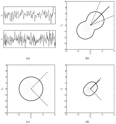
The operation of the linear DSS algorithm is depicted in Fig. 1. Figure 1a shows two sources that have been mixed into Fig. 1b. The mixing vectors have been plotted by the dashed lines. The curve shows the standard deviation of the data projected in different directions. It is evident that the principal eigenvector (solid line) does not separate any of the sources. For that two things would be needed: 1) The mixing vectors should be orthogonal. 2) The eigenvalues should differ. After sphering in Fig. 1c, the basis and sphered mixing vectors are roughly orthogonal. However, any unit-length projection yields unit variance, and PCA still cannot separate the sources. The first source has a somewhat slower temporal evolution and low-pass filtering retains more of that signal, giving it a larger eigenvalue. This is evident in Fig. 1d which shows the denoised data and the first eigenvector, which is now aligned with the (sphered) mixing vector of the slow source. The sources can then be recovered by s=wTX.
There are other algorithms for separating Gaussian sources (Tong et al., 1991; Molgedey and Schuster, 1994; Belouchrani et al., 1997; Ziehe and M¨uller, 1998) and, although functionally dif-ferent, they yield similar results for the example given above. All these algorithms assume that the autocovariance structure of the sources is time-invariant corresponding to Toeplitz autocovariance and filtering matricesΣssand D. In our analysis,Σsscan be any covariance matrix, and only one out
of four examples in Sec. 4.1 has the Toeplitz form.
2.3 Convergence Analysis
In this section, we analyse the convergence properties of DSS algorithms. In the case of linear de-noising, we will refer to well-known convergence properties of the power method (e.g., Wilkinson, 1965). The analysis extends to nonlinear denoising under the assumptions that the mixing model holds and there is an infinite amount of data.
Linear DSS is equivalent to the power method whose convergence is governed by the eigenval-uesλi corresponding to the fixed points w∗i. If some of the eigenvalues are equal (λi=λj, i6= j),
the fixed points are degenerate and there are subspaces of fixed points. In any case, it is possible to choose an orthonormal basis spanned by w∗i. This means that any w can be represented as
w=
∑
i
ciw∗i, (17)
where ci=wTw∗i. With a linear denoising function flin, the unnormalised estimate w+is
w+=XfTlin
∑
icis∗i !
=X
∑
i
cifTlin(s∗i) =
∑
i
ciXfTlin(s∗i) =T
∑
i
s1
s2
−4 −2 0 2 4
−4 −3 −2 −1 0 1 2 3 4
x
1
x 2
(a) (b)
−4 −2 0 2 4
−4 −3 −2 −1 0 1 2 3 4
y
1
y 2
−4 −2 0 2 4
−4 −3 −2 −1 0 1 2 3 4
z
1
z 2
(c) (d)
where λi is the ith eigenvalue corresponding to w∗i and s∗i =w∗iTX. The normalisation step (11)
changes the contributions of the fixed points by equal fractions. After n iterations, the relative contributions of the fixed points thus change from ci
cj into
ciλni
cjλnj.
If there are two fixed points w∗i and w∗j that have identical eigenvaluesλi=λj, the linear DSS cannot separate between the two. This means, for instance, that it is not possible to separate Gaus-sian sources that have identical autocovariance matrices, i.e.,Σsisi=Σsjsj or in other words sources
whose time structures do not differ. Otherwise, as long as ci6=0, the algorithm converges globally
to the source with the largest eigenvalue.
The speed of convergence in the power method (hence in linear DSS) depends linearly on the log-ratio of the largest (absolute) eigenvalues log|λ1|/|λ2|, where|λ1| ≥ |λ2| ≥ |λi|, i=3, . . . ,N. Note that absolute values of the eigenvalues have been used. While the eigenvalues are usually positive, there are cases where negative eigenvalues may exist, for instance in the case of complex data or when using the so-called spectral shift, which is discussed in Sec. 2.5.
The above analysis for linear denoising functions makes no assumptions about the data-generating process. As such it does not extend to nonlinear denoising functions because there can be more or less fixed points than the dimensionality of the data, and the fixed points w∗i are not, in general, orthogonal. We shall therefore assume that the data are generated by independent sources by the model (1) and the assumptions discussed in Sec. 2.1 hold, i.e., the mixing vectors are orthogonal after sphering. Under these assumptions, the orthonormal basis spanned by the mixing vectors corresponds to fixed points of the DSS algorithm. This holds because from the independence of different sources siit follows that
lim
T→∞ 1 T
T
∑
t=1sj(t)ft(si) =0 (19)
for i6= j.
In the linear power method, eigenvaluesλi govern the rate of relative changes of the contribu-tions of individual basis vectors in the estimate. We shall define local eigenvaluesλi(s)which play similar roles in nonlinear DSS. Unlike the constant eigenvaluesλi, the local eigenvalues have dif-ferent values depending on the current source estimate. The formal definition is as follows. Assume that the current weight vector and the subsequent unnormalised new weight vector are
w=
∑
i
ci(s)w∗i (20)
w+=
∑
i
γi(s)w∗i. (21)
The local eigenvalue is defined to be the relative change in the contribution:
γi(s) =T ci(s)λi(s) ⇔ λi(s) = γi(s) T ci(s)
. (22)
The idea of the DSS framework is that the user can tailor the denoising function to the task at hand. The denoising can but need not be based on the E-step (2) derived from a generative model. The purpose of defining the local eigenvalues is to draw attention to the factors influencing separation quality and convergence speed.
means that different sources can have locally the largest eigenvalue. If the adaptation is consistent, i.e.,λi(s)grows monotonically with ci, all stable fixed points correspond to the original sources. In
general, the best separation quality and the fastest convergence is achieved whenλi(s)is very large compared to allλj(s)with j6=i in the vicinity of s∗i.
Sometimes it may be sufficient to separate a signal subspace. Then it is enough for the denoising function to make the eigenvalues corresponding to this subspace large compared to the rest but the eigenvalues do not need to differ within the subspace.
If the mixture model (1) holds and there is an infinite amount of data, the sources can usually be separated even in the linear case because minute differences in the eigenvalues of the sources are sufficient for separation. In practice, the separation is based on a finite number of samples and the ICA model only holds approximately. Conceptually, we can think that there are true eigenvalues and mixing vectors but the finite sample size introduces noise to the eigenvalues and leakage between mixing vectors. In practice the separation quality is therefore much better if the local eigenval-ues differ significantly around the fixed points and this is often easiest to achieve with nonlinear denoising which utilises a lot of prior information.
2.4 Deflation
The classical power method has two common extensions: deflation and spectral shift. They are readily available for the linear DSS since it is equivalent to the power method applied to filtered data via Eq. (2.2). It is also relatively straightforward to apply them in the nonlinear case.
Linear DSS algorithms converge globally to the source whose eigenvalue has the largest magni-tude. Nonlinear DSS algorithms may have several fixed points but even then it is useful to guarantee that the algorithm converges to a source estimate which has not been extracted yet. The deflation method is a procedure which allows one to estimate several sources by iteratively applying the DSS algorithm several times. The convergence to previously extracted sources is prevented by making their eigenvalues zero: worth=w−AATw (Luenberger, 1969), where A now contains the already
estimated mixing vectors.
Note that in this deflation scheme, it is possible to use different kinds of denoising procedures when the sources differ in characteristics. Also, if more than one source is estimated simultaneously, the symmetric orthogonalisation methods proposed for symmetric FastICA (Hyv¨arinen, 1999) can be used. It should be noted, however, that such symmetric orthogonalisation cannot separate sources with linear denoising where the eigenvalues of the sources are globally constant.
2.5 Spectral Shift
As discussed in Sec. 2.2, the matrix multiplication (15) in the power method does not promote the largest eigenvalue effectively compared to the second largest eigenvalue if they have comparable values. The convergence speed in such cases can be increased by so-called spectral shift2 (Wilkin-son, 1965) which modifies the eigenvalues without changing the fixed points. At the fixed point of the DSS algorithm,
λw∗=XfT(s∗)/T. (23)
If the denoising function is multiplied by a scalar, the convergence of the algorithm does not change in any way because the scaling will be overruled by the normalisation step (11). All eigenvalues will be scaled but their ratios, which are what count in convergence, are not affected.
Adding a multiple of s into f(s)does not affect the fixed points because XsT∝w. However the
ratios of the eigenvalues get affected and hence the convergence speed. In summary, f(s)can be replaced by
α(s)[f(s) +β(s)s], (24)
whereα(s)andβ(s)are scalars. The multiplierα(s)is overruled by the normalisation step (11) and has no effect on the algorithm. The termβ(s)s is turned into Tβ(s)w in the re-estimation step (8)
and does affect the convergence speed but not the fixed points (however, it can turn a stable fixed point unstable or vice versa). This is because all eigenvalues are shifted byβ(s):
X[f(s∗) +β(s∗)s∗]T/T =λw∗+β(s∗)w∗= [λ+β(s∗)]w∗.
The spectral shift usingβ(s)modifies the ratios of the eigenvalues and the ratio of the two largest eigenvalues3 becomes |[λ1+β(s)]/[λ2+β(s)]|>|λ1/λ2|, provided that β(s) is negative but not much smaller than−λ2. This procedure can greatly accelerate convergence.
For very negativeβ(s), some eigenvalues will become negative. In fact, ifβ(s)is small enough, the absolute value of the originally smallest eigenvalue will exceed that of the originally largest eigenvalue. Iterations of linear DSS will then minimise the eigenvalue rather than maximise it.
We suggest that it is often reasonable to shift the eigenvalue corresponding to the Gaussian signal νto zero. Some eigenvalues may then become negative and the algorithms can converge to fixed points corresponding to these eigenvalues rather than the positive ones. In many cases, this is perfectly acceptable because, as will be further discussed in Sec. 3.3, any deviation from the Gaussian eigenvalue is indicative of signal. A side effect of a negative eigenvalue is that the estimate w changes its sign at each iteration. This is not a problem but needs to be kept in mind when determining the convergence.
Since the convergence of the nonlinear DSS is governed by local eigenvalues, the spectral shift needs to be adapted to the changing local eigenvalues to achieve optimal convergence speed. In practice, the eigenvalue λν of a Gaussian signal can be estimated by linearising f(s) around the current source estimate s:
f(s+∆s)≈f(s) +∆sJ(s) (25)
λν(s)≈f(s+εν)−f(s)
ε νT/T ≈ ενJ(s)
ε νT/T =νJ(s)νT/T (26) β(s) =E[−λν(s)]≈ −tr J(s)/T (27)
The last step follows from the fact that the elements ofνare mutually uncorrelated and have zero mean and unit variance. Here J(s) denotes the Jacobian matrix of f(s) computed at s. For lin-ear denoising J(s) =D and hence β does not depend on s. If denoising is instantaneous, i.e.,
f(s) = [f1(s(1))f2(s(2)). . .], the shift can be written asβ(s) =−∑t ft0(s(t))/T . This is the spectral
shift used in FastICA (Hyv¨arinen, 1999), but it has been justified as an approximation to Newton’s method and our analysis thus provides a novel interpretation.
Sometimes the spectral shift turns out to be either too modest or too strong, leading to slow convergence or lack of convergence, respectively. For this reason, we suggest a simple stabilisation rule, henceforth called 179-rule: instead of updating w into wnewdefined by Eq. (11), it is updated
into
wadapted=orth(w+γ∆w) (28)
∆w=wnew−w, (29)
whereγis the step size and the orthogonalisation has been added in case several sources are to be extracted. Originallyγ=1, but if the consecutive steps are taken in nearly opposite directions, i.e., the angle between ∆w and ∆wold is greater than 179◦, then γ=0.5 for the rest of the iterations. A stabilised version of FastICA has been proposed by Hyv¨arinen (1999) as well and a procedure similar to the one above has been used. The different speedup techniques considered above, and some additional ones, are studied further by Valpola and S¨arel¨a (2004).
Sometimes there are several signals with similar large eigenvalues. It may then be impossible to use spectral shift to accelerate their separation significantly because of small eigenvalues that would assume very negative values exceeding the signal eigenvalues in magnitude. In that case, it may be beneficial to first separate the subspace of the signals with large eigenvalues from the smaller ones. Spectral shift will then be useful in the signal subspace.
3. Approximation for the Objective Function
The virtue of the DSS framework is that it allows one to develop procedural source separation algorithms without referring to an exact objective function or a generative model. However, in many cases an approximation of the underlying objective function is nevertheless useful. In this section, we propose such an approximation (Sec. 3.1) and discuss its uses, including monitoring (Sec. 3.2) and acceleration of convergence (Sec. 3.3) as well as analysis of separation results (Sec. 3.4).
3.1 The Objective Function of DSS
The power-method version of the linear DSS algorithm maximises the variance ||wTZ||2. When the denoising is performed for the source estimates f(s) =sD, the equivalent objective function is
g(s) =sDsT =s fTlin(s).We propose this formula as an approximation ˆg for the objective function for nonlinear DSS as well:
ˆ
g(s) =s fT(s). (30)
There is, however, an important caveat to be made. Note that Eq. (24) includes the scalar func-tionsα(s)andβ(s). This means that functionally equivalent DSS algorithms can be implemented with slightly different denoising functions f(s)and while they would converge exactly to the same results, the approximation (30) might yield completely different values. In fact, by tuning α(s),
β(s)or both, the approximation ˆg(s)could be made to yield any function which need not have any correspondence to the true g(s).
Let us first check what would be the DSS algorithm maximising ˆg(s). Obviously, the approxi-mation is good if the algorithm turns out to use a denoising similar to f(s). The following Lagrange equation holds at the optimum:
∇w[gˆ(s)−ξTh(w)] =0, (31)
where h denotes the constraints under which the optimisation is performed and ξ are the corre-sponding Lagrange multipliers. In this case, only unit-length projection vectors w are considered, i.e., h(w) =wTw−1=0, and it thus follows that
X∇sgˆT(s)−2ξw=0. (32)
Substituting 2ξ with the appropriate normalising factor which guarantees||w||=1 results in the following fixed point:
w= X∇sgˆ
T(s) ||X∇sgˆT(s)||
. (33)
Using s=wTX and (30), and omitting normalisation yields
w+=X[fT(s) +JT(s)sT], (34) where J is the Jacobian of f. This should conform with the corresponding steps (9) and (10) in the nonlinear DSS which uses f(s)for denoising. This is true if the two terms in the square brackets have the same form, i.e., f(s)∝s J(s).
As expected, in the linear case the two algorithms are exactly the same because the Jacobian is a constant matrix and f(s) =sJ. The denoised sources are also proportional to s J(s)in some special nonlinear cases, for instance, when f(s) =sn.
3.2 Negentropy Ordering
The approximation (30) can be readily used for monitoring the convergence of DSS algorithms. It is also easy to use it for ordering the sources based on their SNR if several sources are estimated using DSS with the same f(s). However, simple ordering based on Eq. (30) is not possible if different denoising functions are used for different sources because the approximation does not provide a universal scaling.
In these cases it is useful to order the source estimates by their negentropy which is a nor-malised measure of structure in the signal. Differential entropy H of a random variable is a measure of disorder and is dependent on the variance of the variable. Negentropy is a normalised quantity measuring the difference between the differential entropy of the component and a Gaussian compo-nent with the same variance. Negentropy is zero for the Gaussian distribution and non-negative for all distributions since among the distributions with a given variance, the Gaussian distribution has the highest entropy.
Calculation of the differential entropy assumes the distribution to be known. Usually this is not the case and estimation of the distribution is often difficult and computationally demanding. Following Hyv¨arinen (1998), we approximate the negentropy N(s)by
be greater than zero, so this is when N(s)should be minimised. A Taylor series expansion of N(s) w.r.t. ˆg(s)around ˆg(ν)yields the approximation (35) as the first non-zero term.
Comparison of signals extracted with different optimisation criteria presumes that the weighting constantsηgare known. We propose thatηgcan be calibrated by generating a signal with a known, nonzero negentropy. Negentropy ordering is most useful for signals which have a relatively poor SNR—the signals with a good SNR will most likely be selected in any case. Therefore we choose our calibration signal to have SNR of 0 dB, i.e., it contains equal amounts of signal and noise in terms of energy: ss= (ν+sopt)/
√
2, where sopt is a pure signal having no noise. It obeys fully
the signal model implicitly defined by the corresponding denoising function f. Since soptandνare
uncorrelated, sshas unit variance. The entropy ofν/ √
2 is
H(ν/√2) =H(ν) +log 1/√2=H(ν)−1/2 log 2.
Since the entropy can only increase by adding a second, independent signal sopt, H(ss)≥H(ν)−
1/2 log 2. It thus holds N(ss) =H(ν)−H(ss)≤1/2 log 2. One can usually expect that sopt has a lot
of structure, i.e., its entropy is low. Then its addition toν/√2 does not significantly increase the entropy. It is therefore often reasonable to approximate
N(ss)≈1/2 log 2=1/2 bit, (36)
where we chose base-2 logarithm yielding bits. Depending on sopt, it may also be possible to
compute the negentropy N(ss)exactly. This can then be used instead of the approximation (36). The coefficients ηg in Eq. (35) can now be solved by requiring that the approximation (35) yields Eq. (36) for ss. This results in
ηg= 1
2(gˆ(ss)−gˆ(ν))2bit (37)
and finally, substitution of the approximation of the objective function (30) and Eq. (37) into Eq. (35) yields the calibrated approximation of the negentropy:
N(s)≈
s fT(s)−νfT(ν)2
2[ssfT(ss)−νfT(ν)]2
bit. (38)
3.3 Spectral Shift Revisited
In Sec. 2.5, we suggested that a reasonable spectral shift is to move the eigenvalue corresponding to a Gaussian signalνto zero. This leads to minimising g(s), when the largest absolute eigenvalue is negative. It does not seem very useful to minimise g(s), a function that measures the SNR of the sources, but as we saw with negentropy and its approximation (35), values g(s)<g(ν)are, in fact, indicative of signal. A reasonable selection forβis thus−λνgiven by (27) which leads linear DSS to extremise g(s)−g(ν)or, equivalently, to maximise the negentropy approximation (35).
possible to extract both super- and sub-Gaussian distributions with a denoising scheme which is designed for one type of distribution only.
Consider for instance f(s) =tanh s which can be used as a denoising function for sub-Gaussian signals while, as will be further discussed in Sec. 4.2.3, s−tanh s=−(tanh s−s) is a suitable denoising for super-Gaussian signals. This shows that depending on the choice of β, DSS can find either sub-Gaussian (β=0) or super-Gaussian (β=−1) sources. With the FastICA spectral shift (27),βwill always lie in the range−1<β≤tanh21−1≈ −0.42. In general,βwill be closer to−1 for super-Gaussian sources which shows that FastICA is able to adapt its spectral shift to the source distribution.
3.4 Detection of Overfitting
In exploratory data analysis, DSS is very useful for giving better insight into the data using a linear factor model. However, it is possible that DSS extracts structures that are due to noise, i.e., the results may be overfits.
Overfitting in ICA has been extensively studied by S¨arel¨a and Vig´ario (2003). It was observed that it typically results in signals that are mostly inactive, except for a single spike. In DSS the type of the overfitted results depends on the denoising criterion.
To detect an overfitted result, one should know what it looks like. As a first approximation, DSS can be performed with the same amount of i.i.d. Gaussian data. Then all the results present cases of overfitting. An even better characterisation of the overfitting results can be obtained by mimicking the actual data characteristics as closely as possible. In that case it is important to make sure that the structure assumed by the signal model has been broken. Both the Gaussian overfitting test and the more advanced test are used throughout the experiments in Secs. 5.2–5.3.
Note that in addition to visual test, the methods described above provide us with a quantitative measure as well. Using the negentropy approximation (38), we can set a threshold under which the sources are very likely overfits and do not carry much real structure. In the simple case of linear DSS, the negentropy can be approximated easily using the corresponding eigenvalue.
4. Denoising Functions in Practice
DSS is a framework for designing source separation algorithms. The idea is that the algorithms differ in the denoising function f(s)while the other parts of the algorithm remain mostly the same. Denoising is useful as such and therefore there is a wide literature of sophisticated denoising meth-ods to choose from (see Anderson and Moore, 1979). Moreover, one usually has some knowledge about the signals of interest and thus possesses the information needed for denoising. In fact, quite often the signals extracted by BSS techniques would be post-processed to reduce noise in any case (see Vigneron et al., 2003). In the DSS framework, the available denoising methods can be directly applied to source separation, producing better results than purely blind techniques. There are also very general noise reduction techniques such as wavelet denoising (Donoho et al., 1995; Vetterli and Kovacevic, 1995) or median filtering (Kuosmanen and Astola, 1997) which can be applied in exploratory data analysis.
relatively specific to almost blind source separation. Many of the denoising functions discussed in this section are applied in experiments in Sec. 5.
The DSS framework has been implemented in an open-source and publicly available MATLAB package (DSS, 2004). The package contains the denoising functions and speedups discussed in this paper and in another paper (Valpola and S¨arel¨a, 2004). It is modular and allows for custom-made functions (denoising, spectral shift, and other parts) to be nested in the core program.
Before proceeding to examples of denoising functions, we note that DSS would not be very useful if very exact denoising would be needed. Fortunately, this is usually not the case and it is enough for the denoising function f(s)to remove more noise than signal (see Hyv¨arinen et al., 2001b, Theorem 8.1), assuming that the independent source model holds. This is because the re-estimation steps (10) and (11) constrain the source s to the subspace spanned by the data. Even if the denoising discards parts of the signal or creates nonexistent signals, re-estimation steps restore them.
If there is no detailed knowledge about the characteristics of the signals to start with, it is useful to bootstrap the denoising functions. This can be achieved by starting with relatively general signal characteristics and then tuning the denoising functions based on analyses of the structure in the noisy signals extracted in the first phase. In fact, some of the nonlinear DSS algorithms can be regarded as linear DSS algorithms where a linear denoising function is adapted to the sources, leading to nonlinear denoising.
4.1 Detailed Linear Denoising Functions
In this section, we consider several detailed, simple but powerful, linear denoising schemes. We introduce the denoisings using the denoising matrix D when feasible. We consider efficient imple-mentation of the denoisings as well.
The eigenvalue decomposition (14) shows that any denoising in linear DSS can be implemented as an orthonormal rotation followed by a point-wise scaling of the samples and rotation back to the original space. The eigenvalue decomposition of the denoising matrix D often offers good intuitive insight into the denoising function as well as practical means for its implementation.
4.1.1 ON/OFF-DENOISING
Consider designed experiments, e.g., in the fields of psychophysics or biomedicine. It is usual to control them by having periods of activity and non-activity. In such experiments, the denoising can be simply implemented by
D=diag(m), (39)
where D refers to the linear denoising matrix in Eq. (9) and
m=
(
1,for the active parts
0,for the inactive parts (40)
This amounts to multiplying the source estimate s by a binary mask,4 where ones represent the active parts and zeroes the non-active parts. Notice that this masking procedure actually satisfies
D=DDT. This means that DSS is equivalent to the PCA applied to denoised Z=XD even with
exactly the same filtering. In practice this DSS algorithm could be implemented by PCA applied to the active parts of the data with the sphering stage would still involving the whole data set.
4.1.2 DENOISINGBASED ONFREQUENCYCONTENT
If, on the other hand, signals are characterised by having certain frequency components, one can transform the source estimate to a frequency space, mask the spectrum, e.g., with a binary mask, and inverse transform to obtain the denoised signal:
D=VΛDVT,
where V is the transform,ΛD is the matrix with the mask on its diagonal, and VT is the inverse transform. The transform V can be implemented for example with the Fourier transform5 or by
discrete cosine transform (DCT). After the transform, the signal is filtered using the diagonal matrix
Λ, i.e., by a point-wise scaling of the frequency bins. Finally the signal is inverse transformed using VT. In the case of linear time-invariant (LTI) filtering, the filtering matrix has a Toeplitz
structure and the denoising characteristics are manifested only in the diagonal matrixΛD, while the transforming matrix V represents a constant rotation. When this is the case, the algorithm can be further simplified by imposing the transformation on the sphered data X. Then the iteration can be performed in the transformed basis. This trick has been exploited in the first experiment of Sec. 5.2.
4.1.3 SPECTROGRAMDENOISING
Often a signal is well characterised by what frequencies occur at what times. This is evident, e.g., in oscillatory activity in the brain where oscillations often occur in bursts. An example of source separation in such data is studied in Sec. 5.2. The time-frequency behaviour can be described by calculating DCT in short windows in time. This results in a combined time and frequency representation, i.e., a spectrogram, where the masking can be applied.
There is a known dilemma in the calculation of the spectrogram: detailed description of the frequency content does not allow detailed information of the activity in time and vice versa. In other words, a large amount of different frequency bins Tf will result in a small amount of time locations
Tt. Wavelet transforms (Donoho et al., 1995; Vetterli and Kovacevic, 1995) have been suggested
to overcome this problem. There an adaptive or predefined basis, different from the pure sinusoids used in Fourier transform or DCT, is used to divide the resources of time and frequency behaviour optimally in some sense. Another possibility is to use the so-called multitaper technique (Percival and Walden, 1993, Ch. 7).
Here we apply an overcomplete-basis approach related to the above methods. Instead of having just one spectrogram, we use several time-frequency analyses with different Tt’s and Tf’s. Then the
new estimate of the projection w+ is achieved by summing the new estimates w+i of each of the time-frequency analyses: w+=∑iw+i .
4.1.4 DENOISING OFQUASIPERIODICSIGNALS
As a final example of denoising based on detailed source characteristics, consider Fig. 2a. Let us assume to be known beforehand that the signal s has a repetitive structure and that the average
repetition rate is known. The quasi-periodicity of the signal can be used to perform DSS to get a better estimate. The denoising proceeds as follows:
−5 0 5 (a)
(b)
−5 0 5 (c)
−5 0 5 (d)
0 500 1000 1500
−10 0 10 (e)
Figure 2: a) Current source estimate s of a quasiperiodic signal b) Peak estimates c) Average signal save (two periods are shown for clarity). d) Denoised source estimate s+. e) Source
estimate corresponding to the re-estimated wnew.
1. Estimate the locations of the peaks of the current source estimate s (Fig. 2b).
2. Chop each period from peak to peak.
3. Dilate each period to a fixed length L (linearly or nonlinearly).
4. Average the dilated periods (Fig. 2c).
5. Let the denoised source estimate s+ be a signal where each period has been replaced by the averaged period dilated back to its original length (Fig. 2d).
The re-estimated signal in Fig. 2e, based on the denoised signal s+, shows significantly better SNR compared to the original source estimate s, in Fig. 2a.
This averaging is a form of linear denoising since it can be implemented as matrix multiplica-tion. Furthermore, it presents another case in addition to the binary masking, where DSS is equiva-lent to the power method even with exactly the same filtering. It would not be easy to see from the denoising matrix D itself that D=DDT. However, this becomes evident should one consider the
averaging of source estimate s+(Fig. 2d) that is already averaged.
4.2 Denoising Based on Estimated Signal Variance
In the previous section, several denoising schemes were introduced. In all of them, the details of the denoising were assumed to be known. It is as well possible to estimate the denoising specifications from the data. This makes the denoising nonlinear or adaptive. In this section, we consider a particular ICA algorithm in the DSS framework, suggesting modifications which improve separation results and robustness.
4.2.1 KURTOSIS-BASEDICA
Consider one of the best known BSS approaches, ICA by optimisation of the sample kurtosis of the sources. The objective function is then g(s) =∑s4(t)/T−3 ∑s2(t)/T2. Since the source variance has been fixed to unity, we can simply use g(s) =∑s4(t)/T and derive the function f(s) from
gradient ascend. This yields∇sg(s) =4/T s3, where s3= [s3(1)s3(2). . .]. Selecting α(s) =T/4
andβ(s) =0 in Eq. (24) then result in
f(s) =s3. (41)
This implements an ICA algorithm with nonlinear denoising. So far, we have not referred to denois-ing, but a closer examination of Eq. (41) reveals that one can, in fact, interpret s3as being s masked by s2, the latter being a somewhat na¨ıve estimate of signal variance and thus relating to SNR.
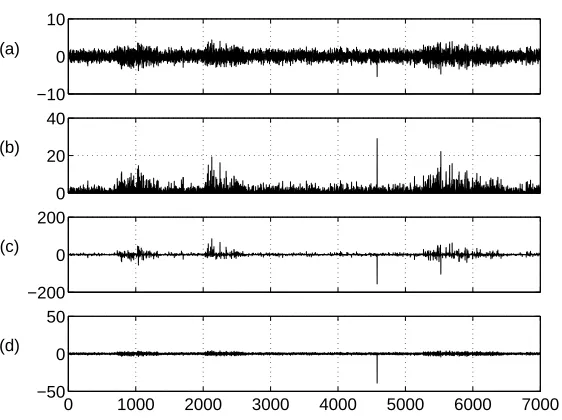
Kurtosis as an objective function is notorious for being prone to overfitting and producing very spiky source estimates (S¨arel¨a and Vig´ario, 2003; Hyv¨arinen, 1998). For illustration of this consider Fig. 3. There one iteration of DSS using kurtosis-based denoising is shown. Assume that via some means, the source estimate shown in Fig. 3a has been reached. The source seems to contain increased activity in three portions (around time instances 1000, 2300 and 6000). As well, it contains a peak roughly at time instance 4700. The signal variance estimate, i.e., the mask is shown in Fig. 3b. While it has boosted somewhat the broad activity compared to the silent parts, the magnification of the peak is far greater. Thus the denoised source estimate s+(Fig. 3c) has nearly nothing else except the peak. The new source estimate snew, based on the new projection wnew, is a clear spike having
little left of the broad activity.
The denoising interpretation suggests that the failure to extract the broad activity is due to a poor estimate of SNR.
4.2.2 BETTERESTIMATE FOR THESIGNALVARIANCE
Let us now consider a related but better founded estimate. Assume that s is composed of Gaussian noise with a constant varianceσ2nand of a Gaussian signal with non-stationary varianceσ2s(t). From Eq. (12) it follows that
s+(t) =s(t) σ
2 s(t) σ2
tot(t)
, (42)
where σ2tot(t) =σ2
s(t) +σ2n is the total variance of the observation. This is also the
maximum-a-posteriori (MAP) estimate.
The kurtosis-based DSS (41) can be obtained from this MAP estimate if the signal variance is assumed to be far smaller than the total variance. In that case it is reasonable to assumeσ2tot to be constant andσ2
s(t) can be estimated by s2(t)−σ2n. Subtraction ofσ2n does not affect the fixed
points as it can be embedded in the termβ(s) =−σ2
nin Eq. (24). Likewise, the division byσ2tot(t)
−10 0 10
(a)
0 20 40
(b)
−200 0 200
(c)
0 1000 2000 3000 4000 5000 6000 7000
−50 0 50
(d)
Figure 3: a) Source estimate s b) Mask s2(t)c) Denoised source estimate s+=f(s) =s3d) Source estimate corresponding to the re-estimated wnew.
Comparison of Eq. (42) and Eq. (41) immediately suggests improvements to the kurtosis-based DSS. For instance, it is clear that if s2(t)is large enough, it is not reasonable to assume thatσ2s(t)is small compared toσ2n(t). Instead, the mask should saturate for large s2(t). This already improves robustness against outliers and alleviates the tendency to produce spiky source estimates.
We suggest the following improvements over the kurtosis-based denoising function (41):
1. The estimates of signal variance and total variance are based on several observations. The rationale of smoothing is the assumption of smoothness of the signal variance. In practice this can be achieved by low-pass filtering the variance of the time, frequency or time-frequency description of s(t), yielding the approximation of total variance.
2. The noise variance is likewise estimated from the data. It should be some kind of soft min-imum of the estimated total variances because the estimate can be expected to have random fluctuations. We suggest the following formula:
σ2
n=C exp
Elog σ2tot(t) +σ2n −σ2n
. (43)
The noise varianceσ2n appears on both sides of the equation, but at the right-hand side, it appears only to prevent rare small values ofσ2
totfrom spoiling the estimate. Hence, we suggest
to use the previously estimated value on the right-hand side. The constant C is tuned such that the formula gives a consistent estimate of the noise variance if the source estimate is, in fact, nothing but Gaussian noise.
has fluctuations, we use a formula which yields zero only when the total variance is zero but which asymptotically approachesσ2tot(t)−σ2
nfor large values of the total variance:
σ2 s(t) =
q σ4
tot(t) +σ4n−σ2n. (44)
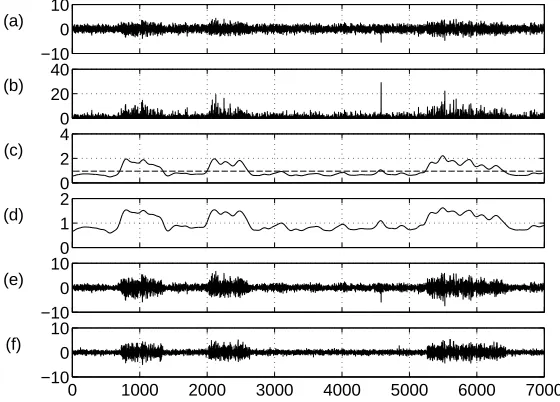
As an illustration of these improvements consider Fig. 4 where one iteration of DSS using the MAP estimate is shown. The first two subplots (Fig. 4a and b) are identical to the ones using kurtosis-based denoising. In Fig. 4c, the variance estimate is smoothed using low-pass filtering. Note that the broad activity has been magnified when compared to the spike around time instance 4700. The noise levelσ2n, calculated using Eq. (43), is shown using a dashed line. Corresponding masking (Fig. 4d) results in a denoised source estimate using Eq. (42), shown in Fig. 4e. Finally, the new source estimate snewis shown after five iterations of DSS in Fig. 4f. DSS using the MAP-based
denoising has clearly removed a considerable amount of background noise as well as the lonely spike.
−10 0 10 (a)
0 20 40 (b)
0 2 4 (c)
0 1 2 (d)
−10 0 10 (e)
0 1000 2000 3000 4000 5000 6000 7000
−10 0 10 (f)
Figure 4: a) Source estimate s b) s2(t)c) Smoothed total variance with the noise level in dashed line d) Denoising mask e) Denoised source estimate s+f) Source estimate after five iterations of DSS.
The exact details of these improvements are not crucial, but we wanted to show that the denois-ing interpretation of Eq. (41) can carry us quite far. The above estimates plugged into Eq. (42) yield a DSS algorithm which is far more robust against overfitting, does not produce the spiky signal estimates and in general yields signals with better SNRs than kurtosis.
points s∗i, the local eigenvalueλi(s∗i)is much larger thanλν, as it should, butλj(s∗i)may be large,
too, which means that the iterations do not remove the contribution of the weaker sources efficiently. Assume, for instance, that two sources have clear-cut and non-overlapping times of strong ac-tivity (σ2s(t)0) and remain silent for most of the time (σ2s(t) =0). Suppose that one source is present for some time at the beginning of the data and another at the end. If the current source estimate is a mixture of both, the mask will have values close to one at the beginning and at the end of the signal. Denoising can thus clean the noise from the signal estimate, but it cannot decide between the two sources.
In this respect, kurtosis actually works better than DSS based on the above improvements. This is because the mask never saturates and small differences in the strengths of the relative contribu-tions of two original sources in the current source estimate will be amplified. This problem only occurs in the saturated regime of the mask and we therefore suggest a simple modification of the MAP estimate (42):
ft(s) =s(t) σ2µ
s (t) σ2
tot(t)
, (45)
where µ is a constant slightly greater or equal to one. Note that this modification is usually needed at the beginning of the iterations only. Once the source estimate is dominated by one of the original sources and the contributions of the other sources fall closer to the noise level, the values of the mask are smaller for the other original sources possibly still present in the estimated source.
Another approach is based on the observation that orthogonalising the mixing vectors A cancels only the linear correlations between different sources. Higher-order correlations may still exist. It can be assumed that competing sources contribute to the current variance estimate: σ2tot(t) =
σ2
s(t) +σ2n+σ2others(t), where σ2others(t) stands for the estimate of total leakage of variance from
the other sources. Valpola and S¨arel¨a (2004) showed that decorrelating the variance-based masks actively promotes the separation of the sources. This bares resemblance to proposals of the role of divisive normalisation on cortex (Schwartz and Simoncelli, 2001) and to the classical ICA method called JADE (Cardoso, 1999).
The problems related to kurtosis are well known and several other improved nonlinear functions
f(s) have been proposed. However, some aspects of the above denoising, especially smoothing of the total-variance estimate s2(t), have not been suggested previously although they arise quite naturally from the denoising interpretation.
4.2.3 TANH-NONLINEARITYINTERPRETED AS SATURATEDVARIANCEESTIMATE
A popular replacement of the kurtosis-based nonlinearity (41) is the hyperbolic tangent tanh(s) operating point-wise on the sources. It is generally considered to be more robust against overfitted and spiky source estimates than kurtosis. By selectingα(s) =−1 andβ(s) =−1, we arrive at
ft(s) =s(t)−tanh[s(t)] =s(t)
1−tanh[s(t)] s(t)
. (46)
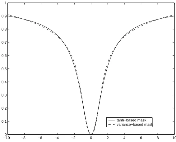
Now the term multiplying s(t)can be interpreted as a mask related to SNR. Unlike the na¨ıve mask s2(t)resulting from kurtosis, the tanh-based mask (46) saturates, though not very fast.
−100 −8 −6 −4 −2 0 2 4 6 8 10 0.1
0.2 0.3 0.4 0.5 0.6 0.7 0.8 0.9 1
tanh−based mask variance−based mask
Figure 5: The tanh-based denoising mask 1−tanh(s)/s is shown together with the variance-based denoising mask proposed here. The parameters in the proposed mask wereσ2n=1 and µ=1.08. We have scaled the proposed mask to match the scale of the tanh-based mask.
can be tuned to the source estimate, µ can be controlled during the iterations and the estimate of the signal variance can be smoothed. These features contribute to the resistance against overfitting and spiky source estimates.
4.3 Other Denoising Functions
There are cases where the system specification itself suggests some denoising schemes. One such case, CDMA transmission, is described in Sec. 5.4. Another example is source separation with a microphone array combined with speech recognition. Many speech recognition systems rely on generative models which can be readily used to denoise the speech signals.
The above is a special case of subspace analysis and there are several other examples where the sources can be grouped to form interesting subspaces. This can be the case, e.g., when all the sources are not independent of each others, but form subspaces that are mutually independent. It may be desirable to use the information in all sources S for denoising any particular source si. This
leads to the following denoising function: s+i =fi(S). Some form of subspace rules can be used to guide the extraction of interesting subspaces in DSS. It is possible to further relax the independence criterion at the borders of the subspaces. This can be achieved by incorporating a neighbourhood denoising rule in DSS, resulting in a topographic ordering of the sources. This suggests a fast fixed-point algorithm that can be used instead of the gradient-descent-based topographic ICA (Hyv¨arinen et al., 2001a).
It is also possible to combine various denoising functions when the sources are characterised by more than one type of structure. Note that the combination order might be crucial for the outcome. This is simply because, in general, fi(fj(s))6=fj(fi(s))where fiand fj present two different linear
or nonlinear denoisings. As an example, consider the combination of the linear on/off-mask (39) and (40), and the nonlinear variance-based mask (45): the noise estimation becomes significantly more accurate when the on/off-masking is performed only after the nonlinear denoising.
Finally, a source might be almost completely known. Then it is possible to apply a detailed matched filter to estimate the mixing coefficients or the noise level. Detailed matched filters have been used in Sec. 5.1 to get an upper limit of the SNRs of the source estimates.
4.4 Spectral Shift and Approximation of the Objective Function with Mask-Based Denoisings
In Sec. 3.1, it was mentioned that a DSS algorithm may work perfectly fine but (30) may still fail to approximate the true objective function ifα(s)andβ(s)are not selected suitably. As an example, consider the mask-based denoisings where denoising is implemented by multiplying the source point-wise by a mask. Without loss of generality, it can be assumed that the data has been rotated with V and the masking operates directly on the source. According to Eq. (30), g(s) =∑ts2(t)m(t), where m(t)is the mask. If the mask is constant w.r.t. s, denoising is linear and Eq. (30) is an exact formula, but let us assume that the mask is computed based on the current source estimate s.
In some cases it may be useful to normalise the mask and this could be implemented in several ways. Some possibilities that may come to mind are to normalise the maximum value or the sum of squared values of the mask. While this type of normalisation has no effect on the behaviour of DSS, it can render the approximation (30) useless. This is because a maximally flat mask usually corresponds to a source with a low SNR. However, after normalisation, the sum of values in the mask would be greatest for a maximally flat mask and this tends to produce high values of the approximation of g(s)conflicting with the low SNR.
As a simple example, consider the mask to be m(t) =s2(t). This corresponds to the kurtosis-based denoising (41). Now the sum of squared values of the mask is∑s4(t), but so is sfT(s). If the mask were normalised by dividing by the sum of squares, the approximation (30) would always yield a constant value of one, totally independent of s.
The above normalisation also has the benefit that the eigenvalue of a Gaussian signal can be expected to be roughly constant. Assuming that the mask m(t)does not depend very much on the source estimate, the Jacobian matrix J(s)of f(s)is roughly diagonal with m(t)as the elements on the diagonal. The trace of J(s) needed for the estimate of the eigenvalue of a Gaussian signal in (27) is then∑tm(t)and the appropriate spectral shift is
β=−1
T
∑
t m(t). (47)The spectral shift can thus be approximated to be constant due to the normalisation.
5. Experiments
In this section, we demonstrate the separation capabilities of the algorithms presented earlier. The experiments can be carried out using the publicly available MATLAB package (DSS, 2004).
The experimental section contains the following experiments: First, in Sec. 5.1, we separate ar-tificial signals with different DSS schemes, some of which can be implemented by FastICA (1998); Hyv¨arinen (1999). Furthermore, we compare the results to one standard ICA algorithm, JADE (1999); Cardoso (1999). In Secs. 5.2–5.3, linear and nonlinear DSS algorithms are applied exten-sively in the study of magnetoencephalograms (MEG). Finally, in Sec. 5.4, recovery of CDMA signals is demonstrated. In each experiment after the case of artificial sources, we first discuss the nature of the expected underlying sources. Then we describe this knowledge in the form of denoising.
5.1 Artificial Signals
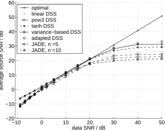
Artificial signals were mixed to compare different DSS schemes and JADE (Cardoso, 1999). Ten mixtures of the five sources were produced and independent white noise was added with different SNRs ranging from nearly noiseless mixtures of 50dB to -10dB, a very noisy case. The original sources and the mixtures are shown in Figs. 6a and 6b respectively. The mixtures shown have SNR of 50 dB.
5.1.1 LINEARDENOISING
In this section, we show how the simple linear denoising schemes described in Sec. 4.1 can be used to separate the artificial sources. These schemes require prior knowledge about the source characteristics.
(a) (b)
Figure 6: (a) Five artificial signals with simple frequency content (signals 1 and 2), simple on/off non-stationarity in time domain (signals 3 and 4) or quasi-periodicity (signal 5). (b) Ten mixtures of the signals in (a).
5.1.2 NONLINEAREXPLORATORYDENOISING
In this section, we describe an exploratory source separation of the artificial signals. One author of this paper gave the mixtures to the other author whose task was to separate the original signals. The testing author did not receive any additional information, so he was forced to apply a blind approach. He chose to use the masking procedure based on the instantaneous variance estimate, described in Sec. 4.2. To enable the separation of both sub- and super-Gaussian sources in the MAP-based signal-variance-estimate denoising, he used the spectral shift (47). To ensure convergence, he used the 179-rule to control the step sizeγ(28). Finally, he did not smooth s2(t)but used it directly as
the estimate of the total instantaneous varianceσ2tot(t).
Based on the separation results of the variance-based DSS, he further devised specific masks for each of the sources. He chose to denoise the first source in frequency domain with a strict band-pass filter around the main frequency. The testing author decided to denoise the second source by a sim-ple denoising function f(s) =sign(s). This makes quite an accurate signal model though it neglects the behaviour of the source in time. The third and fourth signal seemed to have periods of activity and non-activity. He found an estimate for the active periods by inspecting the instantaneous vari-ance estimates s2, and devised simple binary masks. The last signal seemed to consist of alternating positive and negative peaks with a fixed inter-peak-interval as well as some additive Gaussian noise. The signal model was tuned to model the peaks only.
5.1.3 SEPARATIONRESULTS