Maximal Causes for Non-linear Component Extraction

Maximal Causes for Non-linear Component Extraction

J¨org L ¨ucke [email protected]

Maneesh Sahani [email protected]

Gatsby Computational Neuroscience Unit University College London

17 Queen Square London WC1N 3AR, UK

Editor: Yoshua Bengio

Abstract

We study a generative model in which hidden causes combine competitively to produce observa-tions. Multiple active causes combine to determine the value of an observed variable through a max function, in the place where algorithms such as sparse coding, independent component analysis, or non-negative matrix factorization would use a sum. This max rule can represent a more realistic model of non-linear interaction between basic components in many settings, including acoustic and image data. While exact maximum-likelihood learning of the parameters of this model proves to be intractable, we show that efficient approximations to expectation-maximization (EM) can be found in the case of sparsely active hidden causes. One of these approximations can be formulated as a neural network model with a generalized softmax activation function and Hebbian learning. Thus, we show that learning in recent softmax-like neural networks may be interpreted as approxi-mate maximization of a data likelihood. We use the bars benchmark test to numerically verify our analytical results and to demonstrate the competitiveness of the resulting algorithms. Finally, we show results of learning model parameters to fit acoustic and visual data sets in which max-like component combinations arise naturally.

Keywords: component extraction, maximum likelihood, approximate EM, competitive learning,

neural networks

1. Introduction

This form of combination emerges naturally in the context of spectrotemporal masking in mixed audio signals. For image data, occlusion leads to a different combination rule, but one that shares the selection property in that, under constant lighting conditions, the appearance of each observed pixel is determined by a single object.

In parallel to this development of generative approaches, a number of artificial neural network architectures have been designed to tackle the problem of non-linear component extraction, mostly in artificial data (e.g., Spratling and Johnson, 2002; L¨ucke and von der Malsburg, 2004; L¨ucke and Bouecke, 2005; Spratling, 2006), although sometimes in natural images (e.g., Harpur and Prager, 1996; Charles et al., 2002; L¨ucke, 2007). These models often perform quite well with respect to various benchmark tests. However, the relationship between them and the density models that are implicit or explicit in the generative approach has not, thus far, been made clear. We show here that inference and learning in a restricted form of our novel generative model correspond closely in form to the processing and plasticity rules used in such neural network approaches, thus bringing together these two disparate threads of investigation.

The organization of the remainder of this article is as follows. In Section 2 we define the novel generative model and then proceed to obtain the associated parameter update rules in Section 3. In Section 4 we derive computationally efficient approximations to these update rules, in the context of sparsely active hidden causes—that is, when a small number of hidden causes generally suffices to explain the data. In Section 5 we relate a restricted form of the generative model to neural network learning rules with Hebbian plasticity and divisive normalization. Results of numerical experiments in Section 6 show the component extraction performance of the generative schemes as well as a comparison to other algorithms. Finally, in Section 7, we discuss our analytical and numerical results.

2. A Generative Model with Maximum Non-linearity

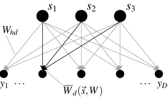
We consider a generative model for D observed variables yd, (d =1, . . . ,D), in which H hidden binary causes sh, (h=1, . . . ,H), each taking the value 0 or 1, compete to determine the value of each observation (see Figure 1). Associated with each pair(sh,yd), is a weight Whd. Given a set of active causes (i.e., those taking the value 1), the distribution of yd is determined by the largest of the weights associated with the active causes and yd.

Much of our discussion will apply generally to all models of this causal structure, irrespective of the details of the distributions involved. For concreteness, however, we focus on a particular choice, in which the hidden variables are drawn from a multivariate Bernoulli distribution; and the observed variables are non-negative, integer-valued and, given the causes, conditionally independent and Poisson-distributed. Thus, collecting all the causes into a single binary vector~s∈ {0,1}H_{, and} all the observed variables into an integer vector~y∈ZD+we have:

p(~s|~π) = H

∏

h=1

p(sh|πh), p(sh|πh) =πs_hh(1−πh)1−sh, (1)

p(~y|~s,W) = D

∏

d=1

p(yd|Wd(~s,W)), p(yd|w) =

wyd yd!

e−w. (2)

s

₁

s

₂

s

₃

· · ·

y

D

W

d

(

~

s

,

W

)

y

1

· · ·

W

hd

Figure 1: A generative model with H =3 hidden variables and D=5 observed variables. The values yd of the observed variables are conditionally independent given the values~s of

the hidden variables. The value yd is drawn from a distribution which is determined by the parameters W1d, W2d, and W3d. For a given binary vector~s these parameters combine

competitively according to the function Wd(~s,W) =maxh{shWhd}.

group these parameters together intoΘ= (~π,W). The function Wd(~s,W)in (2) gives the effective

weight on yd, resulting from a particular pattern of causes~s. Thus, in the model considered here, Wd(~s,W) = max

h {shWhd}. (3)

It is useful to place the model (1)–(3) in context. Models of this general type, in which the obser-vations are conditionally independent of one another given a set of hidden causes, are widespread. They underlie algorithms such as ICA, SC, principal components analysis (PCA), factor analysis (see, e.g., Everitt, 1984), and NMF. In these five cases, and indeed in the majority of such models studied, the effective weights Wd(~s,W)are formed by a linear combination of all the weights that link hidden variables to the observation; that is, Wd(~s,W) =∑hshWhd. Some other models, notably those of Saund (1995) and Dayan and Zemel (1995), have implemented more competitive combina-tion rules, where larger individual weights dominate the effective combinacombina-tion. The present model takes this competition to an extreme, so that only the single largest weight (amongst those associ-ated with active hidden variables) determines the output distribution. Thus, where ICA, PCA, SC, or NMF use a sum, we use a max. We refer to this new generative model as the Maximal Causes Analysis (MCA) model.

{

{

{

{

cause 3

cause 4

A

B

C

cause 2

cause 1 non-linear linear

max

h {shWhd}

∑

h

shWhd

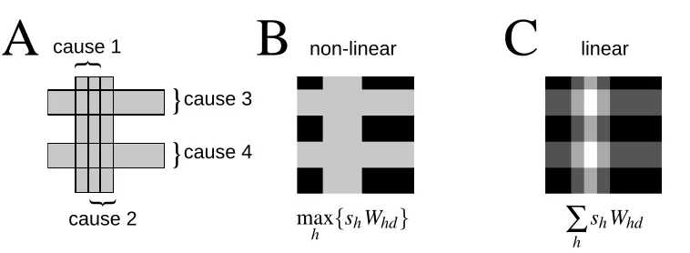
Figure 2: An illustration of non-linear versus linear combination of hidden causes. A Four exam-ples of hidden causes with gray-value 200. B The input image that may result if sources occlude one another. In this case, the correct function Wd(~s,W)(see Figure 1) to combine the hidden causes is the max-operation. C The input image that results if the four causes combine linearly (gray-values are scaled to fill the interval [0,255]). For C, the correct function Wd(~s,W)is linear super-position.

holds approximately. More generally, the maximum combination rule is always closer to the result of occlusion than is the simple sum implied by models such as ICA.

As stated above, although in this paper we focus on the specific distributions given in (1) and (2), much of the analytical treatment is independent of these specific choices. Thus, update rules for learning the weights W from data will be derived in a general form, that can accommodate alternative, non-factored distributions for the binary hidden variables. This general form is also preserved if the Poisson distribution is replaced, for example, by a Gaussian. Poisson variability represents a reasonable choice for the non-negative data considered in this paper, and resembles the cost function introduced by Lee and Seung (1999) for NMF.

3. Maximum Likelihood

Given a set of observed data vectors Y={~y(n)}n=1,...,N, taken to be generated independently from

a stationary process, we seek parameter valuesΘ∗= (~π∗_,W∗_{) that maximize the likelihood of the} data under the generative model of Equations (1) to (3):

Θ∗ _{= argmax}

Θ{

L

(Θ)} with

L

(Θ) =log

p(~y(1), . . . ,~y(N)|Θ).

vectors q(~s(1), . . . ,~s(N)) =∏_nqn(~s(n)). Then the free-energy is defined as:

F

(Θ,q) =

N

∑

n=1 "

∑

~s

qn(~s) hlog p(~y(n)|~s,Θ)

+log p(~s|Θ)i #

+H(q) ≤

L

(Θ), (4)

where H(q) =∑_nH(qn(~s)) =−∑_n∑_~sqn(~s)log(qn(~s))is the Shannon entropy of q. The iterations of EM alternately increase

F

with respect to the distributions qnwhile holdingΘfixed (the E-step), and with respect toΘwhile holding the qnfixed (the M-step). Thus, if we consider a pair of steps beginning from parametersΘ′, the E-step first finds new distributions qnthat depend onΘ′and the observations~y(n), which we write as qn(~s ;Θ′). Ideally, these distributions maximize

F

for fixed Θ′_{, in which case it can be shown that qn(~s ;Θ}′_{) =p(~s|~y}(n)_,Θ′_)and

_F

_(Θ′_{,qn(~s ;Θ}′_{)) =}

_L

_(Θ′_)(Neal and Hinton, 1998). In practice, computation of this exact posterior may be intractable, and it is often replaced by an approximation. After choosing the qn’s in the E-step, we maximize

F

with respect toΘin the M-step while holding the qndistributions fixed. Thus the free-energy can be re-written in terms ofΘandΘ′:

F

(Θ,Θ′) =

N

∑

n=1

∑

~s

qn(~s ;Θ′) hlog p(~y(n)|~s,Θ)

+log p(~s|Θ)i

+ H(Θ′). (5)

where H(Θ′) =∑_nH(qn(~s ;Θ′)). A necessary condition to achieve this maximum with respect to

Wid∈Θ, is that (see Appendix A for details): ∂

∂Wid

F

(Θ,Θ′) =

∑

n

∑

~s

qn(~s ;Θ′) ∂

∂Wid

Wd(~s,W)

y(n)_d −Wd(~s,W)

Wd(~s,W) !

= 0. (6)

Unfortunately, under the max-combination rule of Equation (3), Wd is not differentiable. Instead, we define a smooth function Wρ_d that converges to Wd asρapproaches infinity:

Wρ_d(~s,W) := H

∑

h=1

(shWhd)ρ !1_ρ

⇒ lim ρ→∞W

ρ

d(~s,W) =Wd(~s,W), (7) and replace the derivative of Wd by the limiting value of the derivative of Wρd, which we write as

A

_id (see Appendix A for details):

A

_id(~s,W) := lim

ρ→∞ ∂

∂Wid

Wρ_d(~s,W)

= lim ρ→∞

si(Wid)ρ ∑hsh(Whd)ρ

. (8)

Armed with this definition, a rearrangement of the terms in (6) yields (see Appendix A):

Wid =

∑

n

h

A

_id(~s,W)i_q ny

(n) d

∑

n

h

A

_id(~s,W)i_qn , (9)

whereh

A

_id(~s,W)i_q

n is the expectation of

A

id(~s,W)under the distribution qn(~s ;Θ

′_):

h

A

_id(~s,W)i_q n =

∑

~s

Equation (9) represents a set of non-linear equations (one for each Wid) that defines the necessary conditions for an optimum of

F

with respect to W . The equations do not represent straightforward update rules for Wid because the right-hand-side does not depend only on the old values W′∈Θ′. They can, however, be used as fixed-point iteration equations, by simply evaluating the derivatives

A

id at W′ instead of W . Although there is no guarantee that these iterations converge, if they do converge the corresponding parameters must lie at a stationary point of the free-energy. Numerical experiments described later confirm that this fixed-point approach is, in fact, robust and convergent. Note that the denominator in (9) vanishes only if qn(~s ;Θ′)

A

id(~s,W) =0 for all~s and n (assuming positive weights), in which case (6) is already satisfied, and no update of W is required.

Thus far, we have not made explicit reference to the form of prior source distribution, and so the result of Equation (9) is independent of this choice. For our chosen Bernoulli distribution (1), the M-step is obtained by setting the derivative of

F

with respect toπi to zero, giving (after rearrangement):

πi = 1

N

∑

_n hsiiqn, with hsiiqn =

∑

~s

qn(~s ;Θ′)si. (11)

Parameter values that satisfy Equations (9) and (11), maximize the free-energy given the distribu-tions qn=qn(~s ;Θ′). As stated before, the optimum with respect to q (and therefore, exact opti-mization of the likelihood, since the optimal setting of q forces the free-energy bound to be tight) is obtained by setting the qnto the posterior distributions:

qn(~s ;Θ′) = p(~s|~y(n),Θ′) = p(~s,~y (n)_|Θ′₎

∑

_∼ ~s

p(~s∼,~y(n)|Θ′), (12)

where p(~s,~y(n)|Θ′) = p(~s|~π′_)p(~y(n)_|~s,W′_{), and with the latter distributions given by (1) and (2),} respectively.

Equations (9) to (12) thus represent a complete set of update rules for maximizing the data likelihood under the generative model. The only approximation made to this point is to use the old values W′on the right-hand-side of the M-step equation in (9). We therefore refer to this set of updates as a pseudo-exact learning rule and call the algorithm they define MCAex, with the subscript for exact. We will see in numerical experiments that MCAexdoes indeed maximize the likelihood. 4. E-Step Approximations

The computational cost of finding the exact sufficient statisticsh

A

_id(~s,W)i_q

data vector (note that sparsity here refers to the number of active hidden sources, rather than to their

proportion). The resulting expressions relate to those that would be found by a variational

opti-mization constrained to distributions that are sparse in the sense above, but are not identical. The relationship will be explored further in the Discussion.

To develop the sparse approximations, consider grouping the terms in the expected value of Equation (10) according to the number of active sources in the vector~s:

h

A

id(~s,W)i_qn =

∑

~s

p(~s|~y(n),Θ′)

A

id(~s,W) (13)

=

∑

a

p(~sa|~y(n),Θ′)

A

id(~sa,W) +

∑

a,b a<b

p(~sab|~y(n),Θ′)

A

id(~sab,W) +

∑

a,b,c a<b<c

. . . ,

where ~sa := (0, . . . ,0,1,0, . . . ,0) with only sa=1

~sab := (0, . . . ,0,1,0, . . . ,0,1,0, . . . ,0) with only sa=1, sb=1, a6=b, and~sabcetc. are defined analogously.

Note that

A

id(~0,W) =0 because of (7) and (8). Now, each of the conditional probabilities

p(~s|~y(n),Θ′)implicitly contains a similar sum over~s for normalization:

p(~s|~y(n),Θ′) = 1

Z

p(~s,~y

(n)_|Θ′_),

_Z

_:=

∑

~s

p(~s,~y(n)|Θ′), (14)

and the terms of this sum may be grouped in the same way

Z

:= p(~0,~y(n)|Θ′) +

∑

a

p(~sa,~y(n)|Θ′) +

∑

a,b a<b

p(~sab,~y(n)|Θ′) +

∑

a,b,c a<b<c

p(~sabc,~y(n)|Θ′) +. . . .

Combining (13) and (14) yields:

h

A

_id(~s,W)i_q

n = (15)

∑ap(~sa,~y(n)|Θ′)

A

id(~sa,W) +∑a,b a<b

p(~sab,~y(n)|Θ′)

A

id(~sab,W) +. . .

p(~0,~y(n)_|Θ′_{) +∑}

ap(~sa,~y(n)|Θ′) +∑a,b a<b

p(~sab,~y(n)|Θ′) +. . .

.

A similar grouping of terms is possible for the expectationhshi_qn.

If we now assume that the significant posterior probability mass will concentrate on vectors~s

with only a limited number of non-zero entries, the expanded sums in both numerator and denomi-nator of (15) may be truncated without significant loss. The accuracy of the approximation depends both on the sparsity of the true generative process, and on the distance of the current model param-eters (in the current EM iteration) from the true ones. In general, provided that the true process is indeed sparse, a truncated approximation will become more accurate as the estimated parameters approach their maximum likelihood values. The convergence properties and accuracy of algorithms based on this form of approximation will be tested numerically in Section 6.

4.1 MCA3

In the first approximation, we truncate all but one of the sums that appear in the expansions of h

A

_id(~s,W)i_q

n andhsiiqn after the terms that include three active sources, while truncating the nu-merator ofh

A

_id(~s,W)i_q

n after the two-source terms (see Appendix C for details):

h

A

_id(~s,W)i_q n≈

πiexp(Ii(n)) +

∑

c(c6=i)

πiπcexp(Iic(n))

H

(Wid−Wcd)

1+

∑

h

πhexp(I_h(n)) + 1₂

∑

a,b a6=b

πaπbexp(I_ab(n)) + 1₆

∑

a,b,c a6=b6=c

πaπbπcexp(I_abc(n))

(16)

and hsiiqn≈

πiexp(Ii(n)) +

∑

c(c6=i)

πiπcexp(Iic(n)) + α2

∑

b,c(b6=c6=i)

πiπbπcexp(Iibc(n))

1+

∑

h

πhexp(I_h(n)) + 1₂

∑

a,b a6=b

πaπbexp(I_ab(n)) + 1₆

∑

a,b,c a6=b6=c

πaπbπcexp(I_abc(n))

, (17)

where

πi = πi 1−πi

, I_i(n)=

∑

d

log(Wid)y(n)d −Wid

,

˜

W_dab=max(Wad,Wbd), I_ab(n)=

∑

d

log(W˜_dab)y(n)_d −W˜_dab

,

˜

W_dabc=max(Wad,Wbd,Wcd), Iabc(n)=

∑

d

log(_W˜abc d )y

(n) d −W˜

abc d

,

(18)

and where

H

(x) = 1 for x>0; 1₂ for x=0; 0 for x<0 is the Heaviside function. The above equations have been simplified by dividing both numerator and denominator by terms that do not depend on~s, for example, by∏H_i=1(1−πi)(see Appendix C). Approximations (16) and (17) are used in the fixed-point updates of Equations (9) and (11), where the parameters that appear on the right-hand-side are held at their current values. Thus all parameters that appear on the right-right-hand-side of the approximations take values inΘ′= (~π′_,W′_).

The early truncation of the numerator in (16) improves performance in experiments, partly by increasing competition between causes further, and partly by reducing the contribution of more complex data patterns that are better fit, given the current parameter settings, by three active sources than by two. By contrast, the three-source terms are kept in the numerator of (17). In this case, neglecting complex input patterns as in (16) would lead to greater errors in the estimated source activation probabilitiesπi. Indeed, even while keeping these terms, πi tend to be underestimated if the input data include many patterns with more than three active sources. To compensate, we introduce a factor ofα>1 multiplying the three-source term in (17) (so thatα=1 corresponds to the actual truncated sum), which is updated as described in Appendix C. This scheme yields good estimates ofπi, even if more than three sources are often active in the input data.

4.2 R-MCA2

In the second place, we consider a restriction of the generative model in which (i) all sh are dis-tributed according to the same prior distribution with fixed parameterπ; (ii) the weights Wid associ-ated with each source variable i are constrained to sum to a constant C:

∀i∈ {1, . . . ,H}: πi =π and

∑

d

Wid =C ; (19)

and (iii) on average, the influence of each hidden source is homogeneously covered by the other sources. This third restriction means that each non-zero generating weight W_idgen associated with cause i can be covered by the same number of W_cdgen≥W_idgen:

W_idgen>0 ⇒

∑

c6=i

H

(W_cdgen−W_idgen)≈bi, (20)

where

H

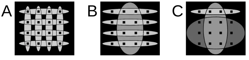
is the Heaviside function and biis the number of causes that can cover cause i. Figure 3

il-B

C

A

Figure 3: A and B show patterns of weights that satisfy the uniformity condition (20) whereas weights in C violate it. Each hidden cause is symbolized by an ellipse, with the gray-level of the ellipse representing the value Wid of each weight within the ellipse. Weights outside the ellipse for each cause are zero (black). The black squares indicate the 4-by-4 grid of observed pixels.

lustrates this condition. Figure 3A,B show weight patterns associated with hidden causes for which the condition is fulfilled; for instance in Figure 3B bi=0 for all causes with horizontal weight pat-terns, while bi=1 for the vertically oriented cause. In Figure 3C the condition is violated. Roughly, these conditions guarantee that all hidden causes have equal average effects on the generated data vectors. They make the development of a more efficient approximate learning algorithm possible but, despite their role in the derivation, the impact of these assumptions is limited in practice, in the sense that the resulting algorithm can perform well even when the input data set violates assump-tions (19) and (20). This is demonstrated in a series of numerical experiments detailed below.

Update rules for the restricted generative model can again be derived by approximate expectation-maximization (see Appendix C). Using both the sum constraint of (19) and the assumption of ho-mogeneous coverage of causes, we obtain the M-step update:

Wid = C

∑

n

h

A

_id(~s,W)i_q ny

(n) d

∑

d′

∑

n

h

A

_id′(~s,W)i_q

n y (n) d′

Empirically, we find that the restricted parameter space of this model means that we can approximate the sufficient statistics h

A

id(~s,W)i_qn by a more severe truncation than before, now keeping two-source terms in the denominator, but only single-two-source terms in the numerator, of the expansion (15). This approximation, combined with the fact that any zero-valued observed patterns (i.e., those with∑_dy(n)_d =0) do not affect the update rule (21) and so can be neglected, yields the expression (see Appendix C):

h

A

_id(~s,W)i_q n ≈

exp(I_i(n))

∑

h

exp(I_h(n)) + π₂

∑

a,b a6=b

exp(I_ab(n)), π := π

1−π, (22)

with abbreviations given in (18). Equations (21) and (22) are update rules for the MCA generative model, subject to the conditions (19) and (20). They define an algorithm that we will refer to as R-MCA2with R for restricted and with 2 indicating a computational cost that grows quadratically with H.

5. Relation to Neural Networks

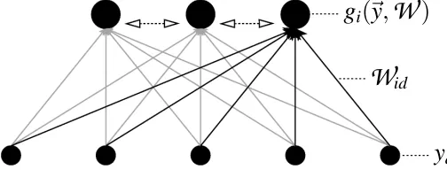
We now relate component extraction as learned within the MCA framework to that achieved by a family of artificial neural networks. Consider the network of Figure 4 which consists of D input variables (or units) with values y1, . . . ,yDand H hidden units with values g1, . . . ,gH. An observation

~y is represented by the values (or activities) of the input units, which act through connections

pa-rameterized by(

W

_id)to determine the activities of the hidden units through an activation function

gi=gi(~y,

W

). These parameters(

W

id)are known as the network (or synaptic) weights.

W

id

g

i(

~

y

,

W

)

y

d

Figure 4: Architecture of a two layer neural network. Input is represented by values y1 to yD of

D input units (small black circles). These values combine with synaptic weights

W

to determine the activities of the hidden units g1to gH (big black circles). The dotted hor-izontal arrows symbolize lateral information exchange that may be required to compute the functions g1to gH. After the giare computed the parameters(

W

id)are modified using a∆-rule.

inputs. A standard choice is the Hebbian∆-rule with divisive normalization:

∆

W

_id = εgi(~y,W)yd and

W

idnew =C

W

_id+∆

W

_id

∑d′(

W

_id′+∆

W

_id′), (23) The normalization step is needed to prevent weights from growing without bound, and the divisive form used here is most common. Here, the constant C defines the value at which ∑_d

W

_id is held constant; it will be related below to the C appearing in Equation 19. Many neural networks with the structure depicted in Figure 4, and that use a learning rule identical or similar to (23), have been shown to converge to weight values that identify clusters in, or extract useful components from, a set of input patterns (O’Reilly, 2001; Spratling and Johnson, 2002; Yuille and Geiger, 2003; L¨ucke and von der Malsburg, 2004; L¨ucke, 2004; L¨ucke and Bouecke, 2005; Spratling, 2006).

The update rule (23) depends on only one input pattern, and is usually applied online, with the weights being changed in response to each pattern in turn. If, instead, we consider the effect of presenting a group of patterns{~y(n)}, the net change is approximately (see Appendix D):

W

_idnew ≈C ∑ngi(~y

(n)_,W)y(n) d ∑d′∑_ng_i(~y(n),W)y(n)_d′

. (24)

Now, comparing (24) to (21), we see that if the activation function of a neural network were cho-sen so that gi(~y(n),W) =h

A

id(~s,W)i_qn, then the network would optimize the parameters of the restricted MCA generative model, with W =

W

(we drop the distinction between

W

and W from now on). Unfortunately, the expectation h

A

_id(~s,W)i_q

n depends on d, and thus exact optimization in the general case would require a modified Hebbian rule. However, the truncated approximation of (22) is the same for all d, and so the changes in each weight depend only on the activities of the corresponding pre- and post-synaptic units. Thus, the Hebbian∆-rule,

∆Wid = εgiyd with gi =

exp(Ii)

∑

h

exp(Ih) + π₂

∑

a,b a6=b

exp(Iab) (25)

(where Ih, Iab, andπare the abbreviations introduced in Equations 18 and 22), when combined with divisive normalization, implements an online version of the R-MCA2 algorithm. We refer to this online weight update rule as R-MCANN(for Neural Network).

Note that the function gi in (25) resembles the softmax function (see, e.g., Yuille and Geiger, 2003), but contains an additional term in the denominator. This added term reduces the change in weights when an input pattern results in more than one hidden unit with significant activity. That is, the system tries to explain a given input pattern using the current state of its model parameters W . If one hidden unit explains the input better than any combination of two units, that unit is modified. If the input is better explained by a combination of two units, the total learning rate is reduced.

6. Experiments

The MCA generative model, along with the associated learning algorithms that have been intro-duced here, are designed to extract component features from non-linear mixtures. To study their performance, we employ numerical experiments, using artificial as well as more realistic data. The artificial data sets are based on a widely-used benchmark for non-linear component extraction, while the more realistic data are taken from acoustic recordings in one case and from natural images in the other. The goals of these experiments are (1) to establish whether the approximate algorithms do indeed increase the likelihood of the model parameters; (2) to test convergence and asymptotic accuracy of the algorithms; (3) to compare component extraction using MCA to other component-extraction algorithms; and (4) to demonstrate the applicability of the model and algorithms to more realistic data where non-linear component combinations arise naturally.

6.1 The Bars Test

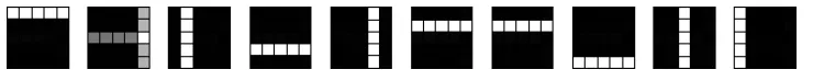
The data sets used in experiments on artificial data were drawn from variants of the “bars test” introduced by F¨oldi´ak (1990). Each data vector represents a grayscale image, with a non-linear combination of randomly chosen horizontal and vertical light-colored bars, each extending all the way across a black background. Most commonly, the intensity of the bars is uniform and equal, and the combination rule is such that overlapping regions remain at the same intensity. This type of data is a benchmark for the study of component extraction with non-linear interactions between hidden causes. Many component-extraction algorithms have been applied to a version of the bars test, including some with probabilistic generative semantics (Saund, 1995; Dayan and Zemel, 1995; Hinton et al., 1995; Hinton and Ghahramani, 1997), as well as many with non-generative objective functions (Harpur and Prager, 1996; Hochreiter and Schmidhuber, 1999; Lee and Seung, 2001; Hoyer, 2004) a substantial group of which have been neurally inspired (F¨oldi´ak, 1990; Fyfe, 1997; O’Reilly, 2001; Charles et al., 2002; Spratling and Johnson, 2002; L¨ucke and von der Malsburg, 2004; L¨ucke and Bouecke, 2005; Spratling, 2006; Butko and Triesch, 2007).

In most of the experiments described here the input data were 25-dimensional vectors, repre-senting a 5-by-5 grid of pixels; that is, D=5×5. There were b possible single bars, some of which were superimposed to create each image. On the 5-by-5 grid there are 5 possible horizontal, and 5 vertical, bar positions, so that b=10. Each bar appears independently with a probabilityπ, with areas of overlap retaining the same value as the individual bars. Figure 5A shows an example set of noisy data vectors constructed in this way.

6.2 Annealing

W1d W2d W3d W4d W5d W6d W7d W8d W9d W10d

100 20

30 0

1

10

Iterations

B

A

Input patterns

Figure 5: Bars test data with b=10 bars on D=5×5 pixels and a bar appearance probability ofπ= ₁₀2. A 24 patterns from the set of N =500 input patterns that were generated according to the generative model with Poisson noise. B Change of the parameters W if MCA3is used for parameter update. Learning stopped automatically after 108 iterations in this trial (see Appendix E).

6.3 Convergence

From a theoretical standpoint, none of the four algorithms MCAex, MCA3, R-MCA2, or R-MCANN, can be guaranteed to maximize the likelihood of the MCA generative model. All of them update the parameters in the M-step using a fixed-point iteration, rather than either maximization or a gradient step. All but MCAex also approximate the posterior sufficient statistics (10). Thus, our first numerical experiments are designed to verify that the algorithms do, in fact, increase parameter likelihood in practice, and that they do converge. For this purpose, it is appropriate to use a version of the bars test in which observations are generated by the MCA model.

Thus, we selected MCA parameters that generated noisy bar-like images. There were 10 hidden sources in the generating model, one corresponding to each bar. The associated matrix of generating weights, Wgen_{, was 10×25, with each row representing a horizontal or vertical bar in a 5-by-5 pixel} grid. The weights W_idgen that correspond to the pixels of the bar were set to 10, the others to 0, so that∑_dW_idgen=50. Each source was active with probabilityπgen_i = 2

bars appearing in each image. We generated N=500 input patterns (each with 25 elements) using Equations (1) to (3); a subset of the resulting patterns is displayed in Figure 5A.

-50

-40

-30

-20

L

(

Θ

)

10

3

-30

-40

-50

1

40

80

120

160

1

2

0

L(Θ)

103

no noise added noise

R-MCA

NN

patterns

103

R-MCA

2

W

gen

,~

π

gen

_MCA

ex

MCA

3

iterations

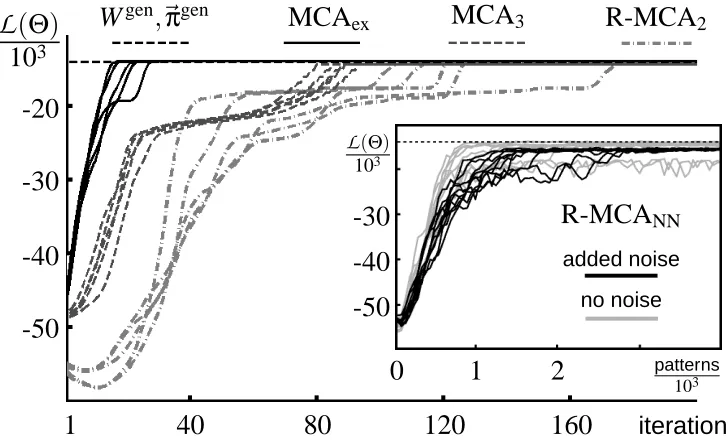
Figure 6: Change of the MCA parameter likelihood under different MCA learning algorithms. Data were generated as in Figure 5. To allow for comparison, the same set of N=500 input patterns was used for all experiments shown. The likelihood of the generating parameters (Wgen,~πgen_{) is shown by the dotted horizontal line. The main axes show likelihood values} of the batch-mode algorithms MCAex, MCA3, and R-MCA2as a function of EM iteration. The inset axes shows likelihood values of the online algorithm R-MCANN as a function of number of input pattern presentations. Patterns were randomly selected from the set of

N=500 inputs, and the parameters were updated for each pattern.

Figure 6 shows the evolution of parameter likelihoods, as a function of iteration, for each of the MCA algorithms, with 5 different choices of initial parameters for each. With the exception of the first few iterations of R-MCA2, the likelihood of the parameters under the batch mode algorithms increased at almost every iteration. The online R-MCANN showed greater fluctuations as updates based on individual data vectors inevitably perturbed the parameter estimates.

these more extensive tests for MCAex due to its long running time (it is also omitted from similar quantitative analyses below).

The two basic observations, that likelihoods generally increased at each iteration and that the batch-mode algorithms all reliably converged, held true for all of the experiments described here and below, even where data were not generated from a version of the MCA model. Thus, we conclude that these algorithms are generally robust in practice, despite the absence of any theoretical guarantees.

6.4 Parameter Recovery

Figure 5B shows the evolution of parameters W , under the approximate MCA3algorithm, showing that the estimated W did indeed converge to values close to the generating parameters Wgen, as was suggested by the convergence of the likelihood to values close to that of the generative parameters. While not shown, the convergence of W under MCAex, R-MCA2 or R-MCANN was qualitatively similar to this sequence.

Clearly, if MCAexfinds the global optimum, we would expect the parameters found to be close to those used for generation. The same is not necessarily true of the approximate algorithms. How-ever, both MCA3 and R-MCA2 did in fact find weights W that were very close to the generating values whenever an obviously poor local optimum was avoided.

In MCA3the average pixel intensity of a bar was estimated to be 10.0±0.5 (standard deviation), taken across all bar pixels in 90 trials where the likelihood increased to a high value. Using R-MCA2 this value was estimated to be 10.0±0.8 (across all bar pixels on 98 high-likelihood trials). Note that the Poisson distribution (2) results in a considerable variance of bar pixel intensities around the mean of 10.0 (compare Figure 5A) which explains the high standard deviation around the relatively precise mean value. The background pixels (original value zero) are estimated to have an intensity of 0.05±0.02 in MCA3and are all virtually zero (all are smaller than 10−56) in R-MCA2. MCA3 also estimates the parameters~π. Because of the finite number of patterns (N=500) we compared the estimates with the actual frequency of occurrence of each bar i: π′_i =(numb of bars i in input)/N.

The mean absolute difference between the estimateπiand the actual probabilityπ′iwas 0.006 (across the 90 trials with high likelihood), which demonstrates the relative accuracy of the solutions, despite the approximation made in Equation (17).

For the neural network algorithm R-MCANN given by (25) we observed virtually the same be-havior as for R-MCA2when using a small learning rate (e.g.,ε=0.1) and the same cooling schedule in both cases (see L¨ucke and Sahani, 2007). The additional noise introduced by the online updates of R-MCANNhad only a negligible effect. For larger learning rates the situation was different, how-ever. For later comparison to noisy neural network algorithms, we used a version of R-MCANN with a relatively high learning rate of ε=1.0. Furthermore, instead of a cooling schedule, we used a fixed temperature T =16 and added Gaussian noise (σ=0.02) at each parameter update: ∆Wid=εgiyd+ση. With these learning parameters, R-MCANN learned very rapidly, requiring fewer than 1000 pattern presentations in the majority of trials. Ten plots of likelihoods against number of presented patterns are shown for R-MCANNin Figure 6 (inset figure, black lines) for the same N=500 patterns as used for the batch-mode algorithms. Because of the additional noise in

W , the final likelihood values were somewhat lower than those of the generating weights. Using

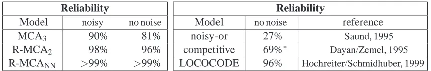
Reliability

Model noisy no noise

MCA3 90% 81%

R-MCA2 98% 96%

R-MCANN >99% >99%

Reliability

Model no noise reference

noisy-or 27% Saund, 1995

competitive 69%∗ Dayan/Zemel, 1995

LOCOCODE 96% Hochreiter/Schmidhuber, 1999

Table 1: Comparison of MCA algorithms with other systems in the standard bars test with b=10 bars (D=5×5,π= 2

10, N=500). For the MCA algorithms reliability values are computed on the basis of 100 trials. Values for these algorithms are also given for the same bars test with Poisson noise. Reliability values for the other systems are taken from the literature. For instance, the model of Hochreiter and Schmidhuber (1999) is reported to fail to extract all bars in one of 25 trials. Two systems, back-propagation (BP) and GeneRec, that are described by O’Reilly (2001) have also been applied to this bars test. In their standard versions, BP and GeneRec achieve 10% and 60% reliability, respectively. Hochreiter and Schmidhuber (1999) report that ICA and PCA extract only subsets of all bars. ∗Trained without bar overlap.

contrast, R-MCANN with noise avoided local optima in all 100 trials. In the following, R-MCANN will therefore refer to the noisy version withσ=0.02 unless otherwise stated.

6.5 Comparison to Other Algorithms—Noiseless Bars

To compare the component extraction results of MCA to that of other algorithms reported in the literature, we used a standard version of the bars benchmark test, in which the bars appear with no noise. The competing algorithms do not necessarily employ probabilistic semantics, and may not be explicitly generative; thus, we cannot compare performance in terms of likelihoods, nor in terms of the accuracy with which generative parameters are recovered. Instead, we adopt a commonly used measure, which asks how reliably all the different bars are identified (see, e.g., Hochreiter and Schmidhuber, 1999; O’Reilly, 2001; Spratling and Johnson, 2002; L¨ucke and von der Malsburg, 2004; Spratling, 2006). For each model, an internal variable (say the activities of the hidden units, or the posterior probabilities of each source being active) is identified as the response to an image. The responses evoked in the learned model by each of the possible single-bar images are then considered, and the most active unit or most probable source corresponding to each bar is identified. If the mapping from single-bar images to the most active internal variable is injective—that is, for each single bar a different hidden unit or source is the most active—then this instance of the model is said to have represented all of the bars. The reliability is the frequency with which each model represents all possible bars, when started from random initial conditions, and given a random set of images generated with the same parameter settings. For the MCA algorithms, the responses are defined to be the approximated posterior values for each possible source vector with only one active source, evaluated at the final parameter values after learning: q(~sh;Θ)≈p(~sh|~ybar,W).

The reliabilities of MCA3, R-MCA2, and R-MCANNas well as some other published component-extraction algorithms are shown in Table 1. These experiments used a configuration of the bars test much as above (D=5×5, b=10, and πgen = 2

in the literature, (e.g., Saund, 1995; Dayan and Zemel, 1995; Hochreiter and Schmidhuber, 1999; O’Reilly, 2001). The bars have a fixed and equal gray-value. We generated N=500 patterns ac-cording to these settings and normalized the input patterns~y(n)to lie in the interval[0,10](i.e., bar pixels have a value of 10 and the background is 0). We considered both the case with Poisson noise (which has been discussed above) and the standard noiseless case. Experiments were run starting from 100 different randomly initialized parameters W . The same algorithms and the same cooling schedule were used (the same fixed T in the case of R-MCANN) to fit patterns with and without noise.

Without noise, MCA3with H=10 hidden variables found all 10 bars in 81 of 100 experiments. R-MCA2 with H=10 found all bars in 96 of 100 experiments. Using the criterion of reliability, R-MCANN performed best and found all bars in all 100 of 100 experiments. This seems likely to result from the fact that the added Gaussian noise, as well as noise introduced by the online updates, combined to drive the system out of shallow optima. Furthermore, R-MCANN was, on average, faster than MCA3and R-MCA2in terms of required pattern presentations. It took fewer than 1000 pattern presentations to find all bars in the majority of 100 experiments,1 _{although in a few trials} learning did take much longer.

On the other hand, MCA3 and R-MCA2 achieved better likelihoods and recovered generative parameters closer to the true values. These algorithms also have the advantage of a well defined stopping criterion. MCA3 learns the parameters of the prior distribution whereas R-MCA2 uses a fixed value. R-MCA2 does, however, remain highly reliable, even when the fixed parameter π differs significantly from the true valueπgen.

Figure 7: A common local optimum found by MCA3in the standard bars test. Two weight patterns reflect the same hidden cause, while another represents the superposition of two causes.

As was the case for the noisy bars, the R-MCA algorithms avoided local optima more often. This may well be a result of the smaller parameter space associated with the restricted model. A common local optimum for MCA3is displayed in Figure 7, where the weights associated with two sources generate the same horizontal bar, while a third source generates a weaker combination of two bars. This local solution is suboptimal, but the fact that MCA3 has parameters to represent varying probabilities for each cause being present, means that it can adjust the corresponding rates to match the data. The fixed setting ofπfor R-MCA would introduce a further likelihood penalty for this solution.

Many component-extraction algorithms—particularly those based on artificial neural networks— use models with more hidden elements than there are distinct causes in the input data (e.g., Charles et al., 2002; L¨ucke and von der Malsburg, 2004; Spratling, 2006). If we use H=12 hidden vari-ables, then all the MCA-algorithms (MCA3, R-MCA2, and R-MCANN) found all of the bars in all of 100 trials.

B

Input patterns with different bar sizes

W after learning (MCA3)

D

W after learning (R-MCANN)

C

W after learning (MCA₃)

Input patterns with overlapping parallel bars

W after learning (MCA3)

Input patterns with 3 bars on average

A

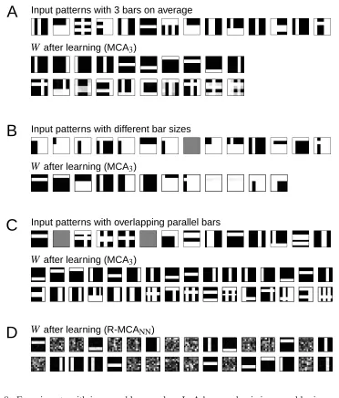
Figure 8: Experiments with increased bar overlap. In A bar overlap is increased by increasing the bar appearance probability toπgen ₌ 3

6.6 Comparison to Other Algorithms—Bar Overlap

For most component-extraction algorithms that have been tested against the bars benchmark, it is difficult to know how specialized they are to the form of this test. The algorithms might, for example, depend on the fact that all bars appear with the same probability, or that they have the same width. Different versions of the bars test have therefore been introduced to probe how generally the different algorithms might succeed. In particular, there has been considerable recent interest in studying robustness to varying degrees of overlap between bars (see, e.g., L¨ucke and von der Malsburg, 2004; L¨ucke, 2004; Spratling, 2006). This is because it is the non-linear combination within the regions of overlap that most distinguishes the bars test images from linear superpositions of sources. In three different experiments we varied the degree of overlap in three different ways. Following Spratling (2006), in all experiments the MCA model had twice as many possible sources as there were bars in the generative input. In all experiments we used the same algorithms, initial conditions, and cooling schedules as described above and in Appendix E. Again, each trial used a newly generated set of training patterns and a different randomly generated matrix W . In the following, reliability values are computed on the basis of 25 trials each.

The most straightforward way to increase the degree of bar overlap is to use the standard bars test with an average of three instead of two bars per image, that is, takeπ= ₁₀3 for an otherwise unchanged bars test with b=10 bars on D=5×5 pixels (see Figure 8A for some examples). When using H=20 hidden variables, MCA3extracted all bars in 92% of 25 experiments. Thus the algorithm works well even for relatively high degrees of superposition. The values of W found in a typical trial are shown in Figure 8A. The parametersW~i= (Wi1, . . . ,WiD)that are associated with a hidden variable or unit are sorted according to the learned appearance probabilitiesπi. Like MCA3, both R-MCA2and R-MCANNwere run without changing any parameters. In the restricted case, this meant that the assumed value for the source probability (π= 2

10) was different from the generating value (πgen= 3

10). Nevertheless, the performance of both algorithms remained better than that of MCA3, with R-MCA2and R-MCANNfinding all 10 bars in 96% and 100% of 25 trials, respectively. We can also choose unequal bar appearance probabilities (cf., L¨ucke and von der Malsburg, 2004). For example, half the bars appeared with probabilityπgen_h = (1+γ)₁₀2 and the other half2 appeared with probabilityπgen_h = (1−γ) 2

10, MCA3 extracted all bars in all of 25 experiments for γ=0.5. Forγ=0.6 (when half the bars appeared 4 times more often than the other half) all bars were extracted in 88% of 25 experiments. Forγ=0.6 R-MCA2 and R-MCANN found all bars in 96% and 100% of 25 experiments respectively. Reliability values for R-MCANNstarted to decrease forγ=0.7 (92% reliability).

As suggested by L¨ucke and von der Malsburg (2004), we also varied the bar overlap in a second experiment by choosing bars of different widths. For each orientation we used two one-pixel wide bars and one three-pixel-wide bar. Thus, for this data set, b=6 and D=5×5. The bar appearance probability wasπ= 2

6, so that an input contained, as usual, two bars on average. Figure 8B shows some examples. MCA3extracted all bars in 84% of 25 experiments for this test. Reliability values decreased for more extreme differences in the bar sizes. R-MCA2 and R-MCANN both found all bars in all 25 trials each. Thus, although the unequal bar sizes violated the assumption∑_dWid=C that was made in the derivation of R-MCA2and R-MCANN, the algorithms’ performance in terms of reliability seemed unaffected.

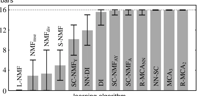
SC -N M FA SC -N M FA Y D I N N -D I SC -N M FY S-N M F N M Fd iv N M Fm se L-N M F 16 12 8 4 0 learning algorithm bars R -M C AN N M C A3 N N -SC R -M C A2

Figure 9: Comparison of MCA3, R-MCA2, and R-MCANNwith other systems in the bars test with increased occlusion (compare Figure 8C and Figure 2). Bars test parameters are D= 9×9, b=16, π= 2

16, and N=400. Data for the non-MCA algorithms are taken from Spratling (2006). The bar heights represent the average numbers of extracted bars in 25 trials. Error bars indicate the largest and the lowest number of bars found in a trial. The algorithms NN-DI and DI are feed-forward neural networks of the type depicted in Figure 4. All other (non-MCA) algorithms are versions of NMF with different objectives and constraints (see Appendix E and Spratling, 2006, for details).

super-numerary units unspecialized can improve the interpretability of the result. When using a higher fixed temperature for R-MCANN all the hidden units represented bars, with some bars represented by more than one unit. However, hidden units that represented more composite inputs, as seen for MCA3, were rarely observed. On the other hand, the parameters found by MCA3 provide an indi-cation of significance of each weight pattern in the appearance probabilitiesπi. Thus, in Figure 8C the appearance probabilities for the first 16 sources are much higher than for the others. The later sources may be interpreted as capturing some of the higher-order structure that results from a finite set of input patterns. In contrast to R-MCA, such higher-order representations need not adversely af-fect the data likelihood because the corresponding appearance probabilities can be relatively small.

A

Generating causes

B

Input patterns

C

W after learning (MCA3)

Figure 10: Experiments with more causes and hidden variables than observed variables. A The 12 patterns used to generate the data. Each is a 1-by-2 pixel bar on a 3-by-3 grid (D=9). B Ten examples of the 500 input patterns generated using the causes shown in A. C Parameters W found in a typical run of MCA3 with H =24. The vectors

~

Wi= (Wi1, . . . ,WiD)appear in order of decreasing learned appearance probabilityπi.

6.7 More Causes than Observed Variables

In the experiments described above, the number of hidden causes was always smaller than the number of observed variables. We next briefly studied the “over-complete” case where data were generated, and models were fit, using more hidden causes than observed variables. We generated

N=500 patterns on a 3-by-3 grid (D=9), using sparse combinations of 12 hidden causes corre-sponding to 6 horizontal and 6 vertical bars, each 1-by-2 pixels in size and thus extending across only a portion of the image (Figure 10A). As in the bars tests above, black was assigned to a value of 0 and white to 10. Patterns were generated without noise, with an average of two bars appearing in each (π= 2

12). Ten such patterns are shown in Figure 10B.

appearance, were associated with more composite patterns. MCA3 extracted all causes in all of 25 trials. R-MCA2also extracted all causes in all of 25 trials, and never represented composite patterns. R-MCANNonly extracted all causes when run at fixed temperatures that were lower than those used for the bars tests above (e.g., T =3), in which case it did so in all of 25 trials. This requirement for a lower temperature was consistent with the observation that a lower data dimension D leads to a decrease in the critical temperatures associated with the algorithms (see Appendix E). For larger values of T (e.g., T =16) R-MCANN did not extract single causes.

6.8 Violations of Model Assumptions

To optimize the likelihood of the data under the MCA generative model, each of the approximate learning algorithms relies on the fact that, under the Bernoulli prior (1), some number of the ob-served data vectors will be generated by only a small number of active sources. To highlight this point we explicitly removed such sparse data vectors from a standard bars test, thereby violating the Bernoulli prior assumption of the generative model. We used bars tests as described above, with b=10 or b=16 bars andπ=2_b, generating N=500 (or more) patterns, in each case by first drawing causes from the Bernoulli distribution (1) and then rejecting patterns in which fewer than m causes were active. As might be expected, when m was 3 or greater the approximate algorithms all failed to learn the weights associated with single causes. However, when only patterns with fewer than 2 bars had been removed, MCA3 was still able to identify all the bars in many of the runs. More precisely, using data generated as above with b=10, m=2 and N=500, MCA3with H=10 hidden variables found all causes in 69 of 100 trials with noisy observations and in 37 of 100 trials without noise (the parameters for MCA3and the associated annealing schedule were unchanged). Note that in these experiments the average number of active causes per input vector is increased by the removal of sparse data vectors. An increase in reliability in the noisy case is consistent with our other experiments. The relatively low reliability seen for noiseless bars in this experiment may be due to the combined violation of both the assumed prior and noise distributions.

As long as the data set did contain some vectors generated by few sources, the learning algo-rithms could all relatively robustly identify the causes given sufficient data, even when the average observation contained many active sources. For instance, in a standard noiseless bars test with

b=16 bars on an 8×8 grid, and N=1000 patterns with an average of four active causes in each (π= 4

16), all three algorithms still achieved high reliability values, using twice as many hidden vari-ables as actual bars (H=32), and using the same parameters as for the standard bars test above. MCA3 found all causes in 20 of 25 trials in these data (80% reliability). Reliabilities of R-MCA2 and R-MCANN(25 trials each) were 76% and 100%, respectively. The reliabilities of all algorithms fell when the data set contained fewer patterns, or when the average number of bars per pattern was larger.

6.9 Applications to More Realistic Data

We study two examples of component extraction in more realistic settings, applying the MCA algo-rithms to both acoustic and image data.

Acoustic data. Sound waveforms from multiple different sources combine linearly, and so are

0 25 50 75 t/ms

0 5

−5

[k] [t] [p]

E

Wafter learning (MCA3)

B

Log-spectrograms of generating phonemes

A

[a0] + [k]

Linear mixture

D

Input data points

C

Generating causes (phoneme waveforms)

A

[a0] [i:] [ c I]

f /kHz

0.1 1.0

0.3 4.0

˜t

[a0_{] [i:] [ c} I] [k] [t] [p]

3 6 9

Figure 11: Application to acoustic data. A Pressure waveforms of six phonemes spoken by a male voice. Axes here, and for the waveform in C, are as shown for [a0] (A is a normalized

amplitude). B The log-spectrograms of the phonemes in A. We use 50 frequency chan-nels and nine time windows (˜t=1, . . . ,9). Axes of all log-spectrograms in the figure are as shown for [a0]. C Waveform of the linear mixture of phonemes [a0] and [k], and

sound. The power of natural sounds in individual time-frequency bins varies over many orders of magnitude, and so is typically measured logarithmically and expressed in units of decibels, giving a representation that is closely aligned with the response of the cochlea to the corresponding sound. In this representation, the combination of log-spectrograms of the different sources may be well approximated by the max rule (R. K. Moore, 1983, quoted by Roweis, 2003). In particular, the logarithmic power distribution, as well as the sub-linear power summation due to phase misalign-ment, both lead to the total power in a time-frequency bin being dominated by the single largest contribution to that bin (see Discussion).

To study the extraction of components from mixtures of sound by MCA, we based the following experiment on six recordings of phonemes spoken by a male voice (see Figure 11A). The phoneme waveforms were mixed linearly to generate N=500 superpositions, with each phoneme appearing in each mixture with probabilityπ= 2₆. Thus each mixture comprised two phonemes on average, with a combination rule that resembled the MCA max-rule in the approximate sense described above.

We applied the MCA algorithms to the log-spectrograms of these mixtures. Figure 11B shows the log-spectrograms of the individual phonemes and Figure 11C shows the log-spectrogram of an example phoneme mixture. We used 50 frequency channels and 9 time bins to construct the log-spectrograms. The resulting values were thresholded and then rescaled linearly so that power-levels across all phonemes filled the interval [0,10], as in the standard bars test. For more details see Appendix E.

The MCA algorithms were used with the same parameter settings as in the bars tests above, except that annealing began at a lower initial temperature (see Appendix E). As in the bars tests with increased overlap, we used twice as many hidden variables (H=12) as there were causes in the input. Figure 11E shows the parameters W learned in one run using MCA3. The parameter vectorsW~i= (Wi1, . . . ,WiD)are displayed in decreasing order of the corresponding learned value of πi. As can be seen, the first six such vectors converged to spectrogram representations similar to those of the six original phonemes. The six hidden variables associated with lower values of πi, converged to weight vectors that represented more composite spectrograms. This result is represen-tative of those found with MCA3. R-MCA2also converged to single spectrogram representations, but tended to represent those single spectrograms multiple times rather than representing more com-posite patterns with the additional components. Results for R-MCANN were very similar to those for R-MCA2when we used a high fixed temperature (see Appendix E for details). For intermedi-ate fixed temperatures, results for R-MCANN were similar to those of the bars test in Figure 8D in that each cause was represented just once, with additional hidden units displaying little structure in their weights. For lower fixed temperatures (starting from T≈40) R-MCANNfailed to represent all causes.

In general, the reliability values of all three algorithms were high. These were measured as described for the bars tests above, by checking whether, after learning, inference based on each individual phoneme log-spectrogram led to a different hidden cause being most probable. MCA3 found all causes in 21 of 25 trials (84% reliability), R-MCA2found all causes in all of 25 trials; as did R-MCANN (with fixed T =70). Reliability for MCA3improved to 96% with a slower cooling procedure (θ_∆W =0.25×10−3; see Appendix E).

Visual data. Finally, we consider a data set for which the exact hidden sources and their mixing rule

C

W

after learning (R-MCA

2

)

Input patches

A

Original image

B

D

Generated patches after learning

from the van Hateren database (Figure 12A) and linearly rescaled so that pixel intensities filled the interval[0,10]. Each data vector was a 10-by-10 pixel patch drawn from a random position in the image (see Figure 12B for some examples).

The image comprised stems and blades of grass which occluded each other. As discussed above (see, e.g., Figure 2), the combination rule for such objects may be well approximated by the max rule of the MCA generative model (at least for the lighting conditions that appear to prevail in Figure 12A). Thus, the MCA learning algorithms may be expected to converge to parameters W that represent intensity images of ‘grass’-like object parts. However, each blade of grass might appear at many different positions within the image patches, rather than at a fixed set of possible locations as in the bars test. Thus to recover these grass-like elements in the MCA causal weights requires the use of models with large numbers of hidden variables (and, correspondingly, many data vectors). For the number of patches and hidden variables required, the cubic cost of MCA3 led to impractically long execution times. In experiments with smaller patch sizes and small H (e.g.,

H=10 or H=20) some weight patterns did converge to represent ‘grass’-like objects, but many converged to less structured configurations.

The computational cost of R-MCA2is smaller and we evaluated trials using H=50 hidden vari-ables and N=5000 10-by-10 patches. R-MCA2 was used with the same parameter setting as for the bars tests above, except for lower initial and final temperatures for annealing (see Appendix E). Figure 12C shows a typical outcome obtained when cooling from T=4.0 to T=1.0. A large num-ber of weight vectors have converged to represent ‘grass’-like object parts, whereas others represent more extensive causes that might be interpreted as capturing background noise. Many of the weight patterns have an orientation similar to the dominant orientation in the original image. Figure 12D shows a selection of patches generated using the learned weights. We used a higher value of C during generation than during learning (the parameter is not learned with R-MCA2), thus globally rescaling the learned weights, so as to reduce the apparent noise level. In experiments where anneal-ing was terminated at T=1.5 (as in the bars test), the resulting weights were generally similar to the ones in Figure 12C, but with a larger proportion of weight vectors showing little structure. Learning with slower annealing did not result in significantly different weights. With fewer than N=5000 patches for training, the weight patterns were less smooth, presumably reflecting overfitting to the subset of data used.

In experiments applying the online algorithm R-MCANN to a set of 5000 10-by-10 patches as above, we found that it would converge to ‘grass’-like weight patterns provided the learning rate (ε in Equation 25) was set to a much lower value than had been used in the bars tests. A lower learning rate corresponds to effectively averaging over a much larger set of input patterns. With ε=0.02 (instead of 1.0 as above), and with noise on the weights (σ) scaled down by the same factor, R-MCANN converged to weights similar to those shown in Figure 12C (for R-MCA2), although a larger number of hidden units showed relatively uniform weight structure. For R-MCANN we used a fixed temperature of T =2.0.

7. Discussion

7.1 Applicability of the Model

The MCA generative model and associated learning algorithms are designed to extract causal com-ponents from input data in which the comcom-ponents combine non-linearly. More precisely, the genera-tive model assumes that the single acgenera-tive cause with the strongest influence on a particular observed variable alone determines its observed value—something we have referred to here as the max-rule for combination. This stands in contrast to other feature extraction models such as PCA, ICA, NMF, or SC, in which the influences of the different causes are summed.

One context in which data with a superposition property very close to the max-rule arise natu-rally is the psychoacoustic combination of sounds. The perception of sound is largely driven by the logarithm of the time-varying intensity within each of a bank of narrow-band frequency channels. The narrow-band, short-time intensity of natural sounds may vary over many orders of magnitude. Further, sounds from different sources may have unrelated phases, and so intensities within each channel will generally add sub-linearly. Thus, even though sound waveforms from different sources combine linearly, the time- and frequency-local intensities, expressed logarithmically (in decibels), are dominated by the loudest of the sounds within each time-frequency bin. Indeed, even if two sounds are of equal loudness, the intensity of the sum is greater than each of them by at most 3 dB. Here, then, the max-rule is a very good approximation to the true generative combination. This observation motivated our use of acoustic data in the experiments shown in Figure 11.

In the image domain, the max-rule’s relevance comes from the fact that it matches the true occlusive combination rule more closely than does the more commonly used sum. This is true both quantitatively (see Figure 2 and the discussion thereof), and also qualitatively, in the sense that both occlusion and the max-rule share a property of exclusiveness—that is, only one of the hidden causes determines the value of each pixel. Numerical experiments on raw image data (Figure 12) demonstrate that plausible generative causes are extracted using the MCA approach. The weight patterns associated with the extracted causes resemble images of the single object parts (blades and stems of grass in our example) that combine non-linearly to generate the image. The MCA approach also holds some potential for component extraction in more low-level image processing, for example, if we assume that each input pixel is generated exclusively by one edge instead of a whole object or object part. The application of MCA might, however, be less straight-forward in this case and presumably requires image preprocessing and perhaps a different noise model.

7.2 Generality of the Framework

Many of the details of the algorithms presented here, as well as many of the experiments, have been based on a specific model in which the hidden variables are drawn from a multivariate Bernoulli dis-tribution (1), and the observations are then Poisson, conditioned on these values (2). These choices are natural ones for non-negative data generated from binary sources (cf., NMF; Lee and Seung, 1999, 2001). However, while the details have largely been omitted for brevity, it is straightforward to incorporate alternative generative distributions within the same framework, and with the same approximations.