Sparse and Unique Nonnegative Matrix Factorization Through Data Preprocessing

Sparse and Unique Nonnegative Matrix Factorization

Through Data Preprocessing

Nicolas Gillis∗ [email protected]

ICTEAM Institute

Universit´e catholique de Louvain B-1348 Louvain-la-Neuve, Belgium

Editor:Inderjit Dhillon

Abstract

Nonnegative matrix factorization (NMF) has become a very popular technique in machine learning because it automatically extracts meaningful features through a sparse and part-based representa-tion. However, NMF has the drawback of being highly ill-posed, that is, there typically exist many different but equivalent factorizations. In this paper, we introduce a completely new way to ob-taining more well-posed NMF problems whose solutions are sparser. Our technique is based on the preprocessing of the nonnegative input data matrix, and relies on the theory of M-matrices and the geometric interpretation of NMF. This approach provably leads to optimal and sparse solutions under the separability assumption of Donoho and Stodden (2003), and, for rank-three matrices, makes the number of exact factorizations finite. We illustrate the effectiveness of our technique on several image data sets.

Keywords: nonnegative matrix factorization, data preprocessing, uniqueness, sparsity, inverse-positive matrices

1. Introduction

Given an m-by-n nonnegative matrix M_≥0 and a factorization rank r, nonnegative matrix

fac-torization (NMF) looks for two nonnegative matricesU andV of dimension m-by-r and r-by-n

respectively such that M_≈UV. To assess the quality of an approximation, a popular choice is

the Frobenius norm of the residual_||M₋UV_||F and NMF can for example be formulated as the

following optimization problem

min

U∈Rm×r_,V∈Rr×n ||M−UV|| 2

F such thatU≥0 andV ≥0. (1)

Assuming thatMis a matrix where each column represents an element of a data set (for example,

a vectorized image of pixel intensities), NMF can be interpreted in the following way. SinceM:j≈

∑rk=1U:kVk j ∀j, each column M:j ofM is reconstructed using an additive linear combination of

nonnegative basis elements (the columns ofU). These basis elements can be interpreted in the same

way as the columns ofM(for example, as images). Moreover, they can only be summed up (since

V is nonnegative) in order to approximate the original data matrixM which leads to a part-based

representation: NMF will automatically extract localized and meaningful features from the data set.

The most famous illustration of such a decomposition is when the columns ofM represent facial images for which NMF is able to extract common features such as eyes, noses and lips (Lee and Seung, 1999); see Figure 8 in Section 6.

NMF has become a very popular data analysis technique and has been successfully used in many different areas such as hyperspectral imaging (Pauca et al., 2006), text mining (Xu et al., 2003), clustering (Ding et al., 2005), air emission control (Paatero and Tapper, 1994), blind source separation (Cichocki et al., 2009), and music analysis (F´evotte et al., 2009).

1.1 Geometric Interpretation of NMF

A very useful tool for understanding NMF better is its geometric interpretation. In fact, NMF is closely related to a problem in computational geometry consisting in finding a polytope nested between two given polytopes. In this section, we briefly recall this connection, which will be exten-sively used throughout the paper.

Let(U,V)be an exact NMF ofM(that is,M=UV,U _≥0 andV _≥0), and let us assume that

no column ofUorMis all zeros; otherwise they can be removed without loss of generality.

Definition 1 (Pullback map) Given an m-by-n nonnegative matrix X without all-zero column, D(X)

is the n-by-n diagonal matrix whose diagonal elements are the inverse of theℓ1-norms of the columns

of X :

D(X)ii=||X:i||−11= m

∑

k=1 |Xki|

!₋1

∀i, D(X)i j=0∀i6=j, (2)

andθ(X) =X D(X) is the pullback map of X so thatθ(X) is column stochastic, that is, θ(X) is nonnegative and its columns sum to one.

We have that (see Chu and Lin, 2008)

M=UV _⇐⇒ θ(M) =MD(M) =U D(U) | {z }

θ(U)

D(U)−1V D(M) | {z }

V′

⇐⇒ θ(M) =θ(U)V′,

whereV′must be column stochastic sinceθ(M)andθ(U)are both column stochastic andθ(M) = θ(U)V′. Therefore, the columns ofθ(M)are convex combinations (linear combinations with

non-negative weights summing to one) of the columns ofθ(U). This implies that

conv(θ(M)) _⊆ conv(θ(U)) _⊆ ∆m_{, (3)}

where conv(X)denotes the convex hull of the columns of matrixX, and∆m_={x∈Rm_{| ∑}m

i xi=

1,xi≥0 1≤i≤m}is the unit simplex (of dimensionm−1). An exact NMFM=UVcan then be

ge-ometrically interpreted as a polytopeT=conv(θ(U))nested between an inner polytope conv(θ(M)) and an outer polytope∆m_.

Hence finding the minimal number of nonnegative rank-one factors to reconstructM

ex-actly is equivalent to finding a polytopeT with minimum number of vertices nested

be-tween two given polytopes: the inner polytope conv(θ(M))and the outer polytope∆m_.

This problem is referred to as the nested polytopes problem (NPP), and is then equivalent to com-puting an exact nonnegative matrix factorization (Hazewinkel, 1984); see also Gillis and Glineur

(2012a) and the references therein. In the remaining of the paper, we will denote NPP(M) the NPP

Remark 2 The geometric interpretation can also be equivalently characterized in terms of cones, see Donoho and Stodden (2003), for which we have

cone(M) _⊆ cone(U) _⊆ Rm+,

where cone(X) =_{x_|x =X a,a_≥0_}. The geometric interpretation based on convex hulls from Equation(3)amounts to the intersection of the cones with the hyperplane_{x_|∑xi=1}(this is the

reason why zero columns of M and U need to be discarded in that case).

1.2 Uniqueness of NMF

There are several difficulties in using NMF in practice. In particular, the optimization problem (1) is NP-hard (Vavasis, 2009), and typically only convergence to stationary points is guaranteed by standard algorithms. There does not seem to be an easy way to go around this (except if the factorization rank is very small, see Arora et al., 2012) since NMF problems typically have many local minima.

Another difficulty is the non-uniqueness: even if one is given an optimal (or good) NMF(U,V)

ofM, there might exist many equivalent solutions(U Q,Q−1V)for non-monomial1matricesQwith

U Q_≥0 andQ−1V _≥0, see Laurberg et al. (2008). Such transformations lead to different

interpre-tations, especially when the supports ofUandV change. For example, in document classification,

each entryMi j of matrixMindicates the ‘importance’ of word iin document j(for example, the

number of appearances of wordiin text j). The factors(U,V)of NMF are interpreted as follows:

the columns ofU represent the topics (that is, bags of words) while the columns ofV link the

doc-uments to these topics. The sparsity patterns ofUandV are then a crucial characteristic since they

indicate which words belong to which topics and which topics is discussed by which documents. Different approaches exist to obtain (more) well-posed NMF problems and most of them are based on the incorporation of additional constraints into the NMF model, for example,

• Sparsity. Require the factors in NMF to be sparse. Under some appropriate assumptions, this

leads to a unique solution (Theis et al., 2005). Geometrically, requiring the matrixU to be

sparse is equivalent to requiring the vertices of the nested polytope conv(θ(U))to be located

on the low-dimensional faces of the outer polytope∆m_{, hence making the problem more well}

posed. In practice, the most popular technique to obtain sparser solutions is to add sparsity

inducing penalty terms, such as aℓ1-norm penalty (Kim and Park, 2007) (see also Section 6).

Another possibility is to use a projection onto the set of sparse matrices (Hoyer, 2004).

• Minimum Volume. Require the polytope conv(θ(U))to have minimum volume (Miao and Qi, 2007; Huck et al., 2010; Zhou et al., 2011) which has a long history in hyperspectral imaging (Craig, 1994). Again, this constraint is typically enforced using a proper penalty term in the objective function. Volume maximization of conv(θ(U))is also possible, leading

to a sparser factorU (since the columns ofU will be encouraged to be on the faces of∆m_),

see Wang et al. (2010), which is essentially equivalent to performing volume minimization for the matrix transpose. In fact, taking the polar of the three polytopes in Equation (3) interchanges the role of the inner and outer polytopes, while the polar of conv(θ(M))is given by conv(θ(MT)), see Gillis (2011, Section 3.6).

• Orthogonality. Require the columns of matrixU to be orthogonal (Ding et al., 2006). Geo-metrically, it amounts to position the vertices of conv(θ(U))on the low-dimensional faces of ∆m_{so that if one of the columns ofθ(U)is not on a facet of∆}m_{(that is,U}

ik>0 for somei,k), then all the other columns ofUmust be on that facet (that is,Uip=0∀p6=k). This condition is rather restrictive, but proved successful in some situations, for example in clustering; see Ding et al. (2005) and Pompili et al. (2011).

1.3 Outline of the Paper

In this paper, we address the problem of uniqueness and introduce a completely new approach to make NMF problems more well posed, and obtain sparser solutions. Our technique is based on a

preprocessing of the input matrix Mto make it sparser while preserving its nonnegativity and its

column space. The motivation is based on the geometric interpretation of NMF which shows that

sparser matrices will correspond to more well-posed NMF problems whose solutions are sparser.

In Section 2, we recall how sparsity ofM makes the corresponding NMF problem more well

posed. In particular, we give a new result linking the support of M and the uniqueness of the

corresponding NMF problem. In Section 3, we introduce a preprocessing

P

(M) =MQofMwhere

Qis an inverse-positive matrix, that is, Qhas full rank and its inverseQ−1 is nonnegative. Hence,

if (U,V′) is an NMF of

P

(M) with

P

(M)_≈UV′, then (U,V′Q−1) is an NMF ofM sinceM=

P

(M)Q−1_≈UV′Q−1 andV′Q−1_≥0. In Section 4, we prove some important properties of the

preprocessing; in particular that it is well-defined, invariant to permutation and scaling, and optimal under the separability assumption of Donoho and Stodden (2003). Moreover, in the exact case for

rank-three matrices (that is, M=UV and rank(M) =3), we show how the preprocessing can be

used to obtain an equivalent NMF problem with a finite number of solutions. In Section 5, we address some practical issues of using the preprocessing: the computational cost, the rescaling of the columns

P

(M)and the ability to dealing with sparse and noisy matrices. In Section 6, we present some very promising numerical experiments on facial and hyperspectral image data sets.

2. Non-Uniqueness, Geometry and Sparsity

Let M_∈Rm+×n and (U,V)∈Rm+×r×Rr+×n be an exact nonnegative matrix factorization ofM=

UV. The minimum r such that such a decomposition exists is the nonnegative rank of M and

will be denoted rank+(M). IfU is not full rank (that is, rank(U)<r), then the decomposition

is typically not unique. In fact, the convex combinations (given byV _≥0) cannot in general be

uniquely determined: the polytopeT =conv(θ(U))has r vertices while its dimension is strictly

smaller thanr₋1 implying that any point in the interior ofT can be reconstructed with infinitely

many convex combinations of thervertices ofT. However, if all columns of conv(θ(M))are located

onk-dimensional faces ofT having exactlyk+1 vertices, then the convex combinations given by

V are unique (Sun and Xin, 2011).

In practice, it is therefore often implicitly assumed that rank+(M) = rank(M) =r hence

rank(U) =r (sinceU has r columns and spans the column space of M of dimension r); see the

discussion by Arora et al. (2012) and the references therein. In this situation, the uniqueness can be characterized as follows:

Theorem 3 (Laurberg et al., 2008) Let (U,V) _∈Rm+×r×Rr+×n and M =UV with rank(M) =

(i) The exact NMF(U,V)of M is unique (up to permutation and scaling).

(ii) There does not exist a non-monomial invertible matrix Q such that U′=U Q_≥0and V′=

Q−1V _≥0.

(iii) The polytopeconv(θ(U))is the unique solution of NPP(M) with r vertices.

It is interesting to notice that the columns ofMcontaining zero entries are located on the bound-ary of the outer polytope∆m_{, and these points must be on the boundary of any solutionT of NPP(M).}

Therefore, ifM contains many zero entries, it is more likely that the set of exact NMF ofM will

be smaller, since there is less degree of freedom to fill in the space between the inner and outer polytopes. In particular, Donoho and Stodden (2003) showed that “requiring that some of the data are spread across the faces of the nonnegative orthant, there is unique simplicial cone”, that is, there is a unique conv(θ(U)).

In the following, based on the assumption that rank(M) =rank+(M), we provide a new

unique-ness result using the geometric interpretation of NMF and the sparsity pattern ofM.

Lemma 4 Let M_∈Rm×n with r=rank(M) =rank+(M), and M have no all-zero columns. If r

columns ofθ(M)coincide with r different vertices of∆m_{∩col(θ(M)), then the exact NMF of M is}

unique.

Proof Let(U,V)_∈Rm+×r×R+r×nbe such thatM=UV. Sincer=rank(M) =rank+(M), we must

have rank(U) =rand col(U) =col(M)(where col(X)denotes the column space of matrixX), hence

conv(θ(M))_⊆conv(θ(U))_⊆∆m_{∩col(θ(M)).}

Sincer columns ofθ(M)coincide withr vertices of∆m_{∩col(θ(M)), we have that conv(θ(U)) =}

conv(θ(M))is the unique solution of NPP(M), and Theorem 3 allows to conclude.

In order to identify such matrices, it would be nice to characterize the vertices of∆m_{∩col(θ(M))} based solely on the sparsity pattern of M. By definition, the vertices of ∆m_{∩col(θ(M))are the} intersection ofr₋1 of its facets, and the facets of∆m_{∩col(θ(M))are given by}

Fi={x∈∆m∩col(θ(M))|xi=0}.

Therefore, a vertex of∆m_{∩col(θ(M))must contain at leastr−1 zero entries. However, this is not}

a sufficient condition because some facets might be redundant, for example, if theith row ofMis

identically equal to zero (for whichFi=∆m∩col(θ(M))) or if theith and jth row ofMare equal to each other (for whichFi=Fj).

Lemma 5 A column of M containing r₋1zeros whose corresponding rows have different sparsity patterns corresponds to a vertex ofconv(θ(M))_∩∆m_.

Proof Letcbe one of the columns ofMwith at leastr₋1 zeros corresponding to rows with different sparsity patterns, that is, there exists

J

_{⊆ {}i_|ci=0}with|

J

|=r−1 such that the rows ofM(

J

,:) have different sparsity patterns. Let alsoFk={x|xJ(k)=0}for 1≤k≤r−1 denote ther−1 facets

r−1 facets are not redundant: for all 1_≤k<p≤r−1, there existxk andxpin conv(θ(M))∩∆m such thatxk∈Fk,xk∈/Fpandxp∈Fp,xp∈/Fk. Because the rows ofM(

J

,:)have different sparsity patterns, for all 1_≤k<p_≤r₋1, there must exist two indiceshandlsuch thatM(

J

(k),h) =0 and

M(

J

(p),h)>0 whileM(

J

(k),l)>0 andM(

J

(p),l) =0. Therefore,θ(M:h)∈Fk,θ(M:h)∈/Fpand θ(M:l)∈Fp,θ(M:l)∈/Fkand the proof is complete.

Theorem 6 Let M_∈Rm×nwith r=rank(M) =rank+(M). If M has r non-zero columns each having

r₋1zero entries whose corresponding rows have different sparsity patterns, then the NMF of M is unique.

Proof This follows directly from Lemma 4 and 5.

Here is an example,

M=



  

0 1 1

0 0 1

1 0 0

1 1 0



  ,

with rank(M) =rank+(M) =3 whose unique NMF is M=MI, whereI is the identity matrix of

appropriate dimension. Other examples include matrices containing anr-by-rmonomial submatrix;

see also Kalofolias and Gallopoulos (2012) and the references therein. It is interesting to notice that this result implies that the only 3-by-3 rank-three nonnegative matrices having a unique exact NMF are the monomial matrices (permutation and scaling of the identity matrix) since all other matrices

have at least two distinct exact NMF:M=MI=IM.

Finally, although sparsity is neither a necessary (see Remark 7 below) nor a sufficient condition for uniqueness (except in some cases, see for example Theorem 6 or Donoho and Stodden, 2003),

the geometric interpretation of NMF shows that sparser matricesMlead to more well-posed NMF

problems. In fact, many points of the inner polytope in NPP(M) are located on the boundary of the

outer polytope∆m_{. Moreover, because the solutionT must contain these points, it will have zero}

entries as well. In particular, assumingMdoes not contain a zero column, it is easy to check that

forM=UVwe have

Mi j=0 ⇒ ∃ksuch thatUik=0.

Remark 7 Having many zero entries in M is not a necessary condition for having an unique NMF. In fact, Laurberg et al. (2008) showed that there exist positive matrices with unique NMF. However, for an NMF (U,V) to be unique, the support of each column of U (resp. row of V ) cannot be contained in the support of any another column (resp. row) so that each column of U (resp. row of V ) must have at least one zero entry. In fact, assume the support of the kth column of U is contained in the support of lth column. Then notingp¯=argmin_{{p|U(p,k)6=0}U}U(_(p,kp,l)₎,ε=_UU(_(p,kp,l_¯¯ )₎, and

Dkl=−ε, Dii=1∀i, Di j=0otherwise,

one can check that D−1is as follows

D−_kl1=ε, D−_ii1=1_∀i, D−_{i j}1=0otherwise,

3. Preprocessing for More Well-Posed and Sparser NMF

In this section, we introduce a completely new approach to obtain more well-posed NMF problems whose solutions are sparser. As it was shown in the previous paragraph, this can be achieved by

working with sparser nonnegative matrices. Hence, we look for ann-by-nmatrixQsuch thatMQ=

M′ is nonnegative, sparse and Qis inverse-positive. In other words, we would like to solve the

following problem:

min

Q∈Rn×n||MQ||0 such that MQ≥0 andQ

−1_{≥0, (4)}

where_||X_||0is theℓ0-‘norm’ which counts the number of non-zero entries inX. Assuming we can

solve (4) and obtain a matrixM′=MQ, then any NMF(U,V′)ofM′ withM′_≈UV′ gives a NMF

forM. In fact,

M = M′Q−1 _≈ UV′Q−1 = UV, whereV =V′Q−1_≥0,

for which we have

||M₋UV_||F =||M′Q−1−UV′Q−1||F =||(M′−UV′)Q−1||F ≤ ||M′−UV′||F||Q−1||2.

In particular, if the NMF of M′ is exact, then we also have an exact NMF for M=M′Q−1=

UV′Q−1=UV. The converse direction, however, is not always true. We return to this point in

Section 4.3.

In the remaining of this section, we propose a way to finding approximate solutions to problem (4). First, we briefly review some properties of inverse-positive matrices (Section 3.1) in order to

deal with the constraintQ−1_≥0. Then, we replace theℓ0-‘norm’ with theℓ2-norm and solve the

corresponding optimization problem using constrained linear least squares (Section 3.2).

3.1 Inverse-Positive Matrices

In this section, we recall the definition of three types of matrices: Z-matrices, M-matrices and inverse-positive matrices, briefly recall how they are related and provide some useful properties. We refer the reader to the book of Berman and Plemmons (1994) and the references therein for more details on the subject.

Definition 8 An n-by-n Z-matrix is a real matrix with non-positive off-diagonal entries.

Definition 9 An n-by-n M-matrix is a real matrix of the following form:

A=sI₋B, s>0, B_≥0,

where the spectral radius2ρ(B)of B satisfies s_≥ρ(B).

It is easy to see that an M-matrix is also a Z-matrix.

Definition 10 An n-by-n matrix Q is inverse positive if and only if Q−1exists and Q−1is nonnega-tive. We will denote this set

I P

n:

I P

n=_{Q_∈Rn×n|Q is full rank and Q−1_≥0_}.

It can be shown that inverse-positive Z-matrices are M-matrices:

Theorem 11 (Berman and Plemmons 1994, Theorem 2.3) Let A be a Z-matrix. Then the follow-ing conditions are equivalent :

• A is an invertible M-matrix.

• A=sI₋B with B_≥0, s>ρ(B).

• A_∈

I P

n.

Here is another well-known theorem in matrix theory which will be useful, see Taussky (1949) and the references therein.

Definition 12 An n-by-n matrix A is irreducible if and only if there does not exist an n-by-n permu-tation matrix P such that

PTAP=

B C

0 D

,

where B and D are square matrices.

Definition 13 An n-by-n matrix A is irreducibly diagonally dominant if A is irreducible,

|Aii| ≥

∑

k6=i

|Aki|, for i=1,2, . . . ,n,

and the inequality is strict for at least one i.

Theorem 14 If A is irreducibly diagonally dominant, then A is nonsingular.

3.2 Constrained Linear Least Squares Formulation for(4)

Theℓ0-‘norm’ is of combinatorial nature and typically leads to intractable optimization problems.

The standard approach is to use theℓ1-norm instead but we propose here to use theℓ2-norm. The

reason is twofold:

• When looking at the structure of problem (4), we observe that any (reasonable) norm will

induce solutions with zero entries. In fact, some of the constraintsMQ_≥0 will always be

active at optimality because of the objective function_||MQ_||.

• Theℓ2-norm is smooth hence its optimization can be performed more efficiently.3 We then would like to solve

min

Q_∈I Pn||MQ||

2

F such that MQ≥0. (5)

Optimizing over the set of inverse-positive matrices

I P

n seems to be very difficult. At least,

de-scribing

I P

nexplicitly as a semi-algebraic set requires aboutn2polynomial inequalities of degree

3. Because of the constraintMQ≥0, theℓ1-norm problem can actually be decoupled intonlinear programs (LP) in

up ton, each with up ton! terms. However, we are not aware of a rigorous analysis of the complexity of this type of problems; this is a topic for further research.

For this reason, we will restrict the search space to the subset of Z-matrices, that is,

inverse-positive matrices of the formQ=sI₋B, wheres is a nonnegative scalar,I is the identity matrix

of appropriate dimension andBis a nonnegative matrix such that ρ(B)<s, see Section 3.1. It is important to notice that

• The scalarscannot be chosen arbitrarily. In fact, makingsgo to zero andB=0, the objective function value goes to zero, which is optimal for (5). The same degree of freedom is in fact

present in the original problem (4) sinceQandαQfor anyα>0 are equivalent solutions.

Therefore, without loss of generality, we fixsto one .

• The diagonal entries ofBcannot be chosen arbitrarily. In fact, takingBarbitrarily close (but smaller) to the identity matrix, the infimum of (5) will be equal to zero. We then have to set an upper bound (smaller than one) for the diagonal entries ofB. It can be checked that this upper bound will always be attained (because of the minimization), and that the optimal solutions corresponding to different upper bounds will be multiples of each other. We therefore fix the bound to zero implyingBii=0 for alliso thatQii=1 for alli.

Finally, we would like to solve

min

Q∈Qn ||MQ|| 2

F such that MQ≥0,

where

Q

n=_{Q_∈Rn×n|Q=I₋B,B_≥0,Bii=0∀i,ρ(B)<1} ⊂

I P

n.

SinceMQ=M(I₋B)_≥0, this problem is equivalent to

min B∈Rn×n

n

∑

i=1

M:i−

∑

k6=i

M:kBki 2 2

such that M_≥MB, (6)

ρ(B)<1,

Bii=0∀i,B≥0.

Without the constraint on the spectral radius ofB, this is a constrained linear least squares problem (CLLS) in

O

(n2)variables and

O

(n2+mn)constraints. Theith column ofM′=MQ, which is the

preprocessed version ofM, will then be given by the following linear combination

M_:i′ =MQ:i=M:i− n

∑

k=1

M:kBki≥0, whereBki≥0∀i,k and Bii=0. (7)

This means that we will subtract from each column ofM a nonnegative linear combination of the

other columns ofMin order to maximize its sparsity while keeping its nonnegativity. Intuitively,

this amounts to keeping only the non-redundant information from each column ofM(see Section 6

3.2.1 RELAXING THECONSTRAINT ON THESPECTRALRADIUS

In general, there is no easy way to deal with the non-convex constraint ρ(B)<1. In particular, this constraint may lead to difficult optimization problems, for example, finding the nearest stable matrix to an unstable one:

min

X ||X−A|| such that ρ(X)≤1,

see Polyak and Shcherbakov (2005) and the references therein. This means that even the projection on the feasible set is non-trivial.

However, we will prove in Section 4 that if the columns of Mare not multiples of each other,

then any optimal solution of problem (6) without the constraint on the spectral radius ofB, that is, any optimal solutionB∗of

min B∈Rn+×n

n

∑

i=1

M:i−

∑

k6=i

M:kBki 2

2 such that M≥MB,Bii=0∀i, (8)

automatically satisfies ρ(B∗)<1 (Theorem 21). Hence, the approach may only fail when there

are repetitions in the data set. The reason is that when a column is multiple of another one, say

M:i=αM:j fori6= jandα>0, then takingBi j =α(0 otherwise for that column) gives MQ:i=

M:i−αM:j=0 and similarly forM:j. Hence we have lost a component in our data set and potentially

produce a lower rank matrixMQ. In practice, it will be important to make sure that the columns of

Mare not multiples of each other (even though it is usually not the case for well-constructed data

sets).

4. Properties of the Preprocessing

In the remainder of the paper, we denote

B

∗(M)the set of optimal solutions of problem (8) for the

data matrixM, and

P

the preprocessing operator defined as

P

:Rm+×n→R+m×n:M7→

P

(M) =M(I−B∗), whereB∗∈

B

∗(M).

In this section, we prove some important properties of

P

and

B

∗(M):

• The preprocessing operator

P

is well-defined (Theorem 15).

• The preprocessing operator

P

is invariant to permutation and scaling of the columns of M

(Lemma 16).

• If the columns ofθ(M)are distinct, thenρ(B∗)<1 for anyB∗_∈

B

∗(M)(Theorem 21). • If the vertices of conv(θ(M))are distinct then

– There existsB∗_∈

B

∗(M)such thatρ(B∗)<1 (Corollary 22).

– rank(

P

(M)) =rank(M)and rank+(

P

(M))≥rank+(M)(Corollary 19).

• If the matrixM is separable, then the preprocessing allows to recover a sparse and optimal

solution of the corresponding NMF problem (Theorem 24). In particular, it is always optimal for rank-two matrices (Corollary 25).

• If the matrix has rank-three, then the preprocessing yields an instance in which the number of

4.1 General Properties

A crucial property of our preprocessing is that it is well-defined.

Theorem 15 The preprocessing

P

(M)is well-defined: for any B∗_1∈

B

∗(M),B∗_2∈

B

∗(M), we have M(I₋B∗₁) =M(I₋B∗₂) =

P

(M).

Proof Problem (8) can be decoupled intonindependent CLLS (one for each column ofM) of the form:

min b_∈Rn+−1

kd₋Cb_k2such thatCb_≤d, (9)

which is equivalent to

min b∈Rn+−1,y∈Rm

kd₋y_k2such thaty_≤d,y=Cb.

The result follows from the fact that theℓ2projection onto a polyhedral set (actually any convex set) yields a unique point.

Another important property of the preprocessing is its invariance to permutation and scaling of

the columns ofM.

Lemma 16 Let M be a nonnegative matrix and P be a monomial matrix. Then,

P

(MP) =

P

(M)P.

Proof We are going to show something slightly stronger; namely thatB∗is an optimal solution of (8) for matrixMif and only ifP−1B∗Pis an optimal solution of (8) for matrixMP:

B∗ _∈

B

∗(M) _⇐⇒ P−1B∗P _∈

B

∗(MP).

First, note that Bis a feasible solution of (8) forMif and only if P−1BPis a feasible solution of

(8) forMP. In fact, nonnegativity ofB and its diagonal zero entries are clearly preserved under

permutation and scaling while

M_≥MB _⇐⇒ MP_≥MBP _⇐⇒ MP_≥(MP)(P−1BP).

Hence there is one-to-one correspondence between feasible solutions of (8) forMand (8) forMP.

Then, letB∗ be an optimal solution of (8). Because (8) can be decoupled into nindependent

CLLS’s, one for each column ofB(cf. Equation (9)), we have

||M:i−MB∗:i||22≤ ||M:i−MB:i||22, ∀i,

for any feasible solutionBof (8). Letting p_∈Rn+ be such that pi is equal to the non-zero entry of theith row ofP, we have

∑

i

p2_i||M:i−MB∗:i||22=

∑

i

||M:ipi−MPP−1B∗:ipi||22 =_||MP₋MPP−1B∗P_||2_F

≤

∑

i

for any feasible solutionB′=P−1BPof (8) forMP. This provesB∗∈

B

∗(M)_⇒P−1B∗P∈

B

∗(MP).

The other direction follows directly by using the permutationP−1on the matrixMP.

It is interesting to observe that if a column ofMbelongs to the convex cone generated by the

other columns, then the corresponding column of

P

(M)is equal to zero.

Lemma 17 Let

J

=_{1,2, . . . ,n_}\{i_}. Then

P

(M):i=0if and only if M:i∈cone(M(:,

J

)).

Proof We have that

P

(M):i=M:i−

∑

k6=i

B∗_kiM:k=0, B∗ki≥0 ⇐⇒ M:i=

∑

k6=i

B∗_kiM:k, B∗ki≥0.

The preprocessed matrix

P

(M) may contain all-zero columns, for which the function θ(.) is

not defined (cf. Definition 1). We extend the definition to matrices with zero columns as follows:

θ(X) is the matrix whose columns are the normalized non-zero columns of X, that is, letting Y

be the matrixX where the non-zero columns have been removed, we defineθ(X) =θ(Y). Hence

conv(θ(X))denotes the convex hull of the normalized non-zero columns ofX.

Another straightforward property is that the preprocessing can only inflate the convex hull de-fined by the columns ofθ(M).

Lemma 18 Let M_∈Rm+×n. If the vertices ofconv(θ(M))are non-repeated, then

conv(θ(M)) _⊆ conv(θ(

P

(M))) _⊆ ∆m_∩col(θ(M)).

Proof By construction, since

P

(M) =MQ, col(θ(

P

(M)))_⊆col(θ(M))and conv(θ(

P

(M)))_⊆ ∆m_{∩col(θ(M)). Let ibe the index corresponding to a vertex ofθ(M) and}

_J

_{={1,2, . . . ,n}\{i}.} Because vertices ofθ(M)are non-repeated, we haveM:i∈/conv(θ(M(:,

J

))), while

P

(M):i=M:i−

∑

k6=i

bkiM:k ⇐⇒ M:i=

P

(M):i+

∑

k6=i

bkiM:k.

HenceM:i∈conv(θ([

P

(M):iM(:,

J

)])), which implies that

conv(θ(M))_⊆conv(θ([

P

(M):iM(:,

J

)])),

so that replacingM:i by

P

(M):iextends conv(θ(M)). Since this holds for all vertices, the proof is complete.

Corollary 19 Let M_∈Rm+×n. If no column of M is multiple of another column, then

Proof Without loss of generality, we can assume that M does not have a zero column. In fact, a preprocessed zero column remains zero while it cannot influence the preprocessing of the other columns (see Equation (7)). Then, by Lemma 18, we have

conv(θ(M)) _⊆ conv(θ(

P

(M))) _⊆ ∆m_∩col(θ(M)),

implying rank+(

P

(M))≥rank+(M)and rank(

P

(M)) =rank(M).

Another way to prove this result is to use Corollary 22 (see below) guaranteeing the existence

of an inverse-positive matrix Q such that

P

(M) =MQ which implies rank(

P

(M)) = rank(M).

Moreover, any exact NMF(U,V)_∈Rm×r×Rr×nof

P

(M)givesM=UV Q−1hence rank+(M)≤

rank+(

P

(M)).

We now prove that if no column of M is multiple of another column (that is, the columns of

θ(M) are distinct) then ρ(B∗)<1 for anyB∗∈

B

∗(M) whenceQ=I−B∗ is an inverse positive matrix.

Lemma 20 Let A be a column stochastic matrix and Q=I₋B where B_≥0and Bii=0for all i be

such that AQ≥0. Then,

∑

k

Bki≤1, ∀i,

so that Q is diagonally dominant. Moreover, if A:i∈/conv(A(:,

J

))where

J

={1,2, . . . ,n}\{i}, then

∑

k

Bki<1.

Proof By assumption, we have for alli

A:i≥AB:i=

∑

k

A:kBki,

which implies

1=_||A:i||1≥ ||AB:i||1=||

∑

k

A:kBki||1=||B:i||1=

∑

k

Bki,

becauseA andBare nonnegative. Moreover, ifA:i∈/conv(A(:,

J

)), then there exists at least one index jsuch thatAji>Aj:B:i(Lemma 17) so that the above inequality is strict.

Theorem 21 If no column of M is multiple of another column, then any optimal solution B∗of (8)

satisfiesρ(B∗)<1whence Q=I₋B∗is inverse positive.

Proof By Theorem 11,ρ(B∗)<1 if and only if Q=I₋B∗ is inverse positive if and only ifQis

a nonsingular M-matrix. Let us then show thatQis a nonsingular M-matrix. First, we can assume

without loss of generality that

• MatrixMdoes not contain a column equal to zero. In fact, ifM does, say the first column

is equal to zero, then we must have B:1=0 (since M:1 ≥MB:1 and there is not other zero

• The columns ofM sum to one. In fact, lettingP=D(M)be defined as in Equation (2), by Lemma 16,B∗is an optimal solution forMif and only ifP−1B∗Pis an optimal solution for

MP. SinceB∗andP−1B∗Pshare the same eigenvalues,ρ(B∗)<1 _⇐⇒ ρ(P−1B∗P)<1. • LetB_∈

B

∗(M),Q=I₋B∗, andPbe a permutation matrix such that

PTQP=       

Q(1) Q(12) Q(13) . . . Q(1k)

0 Q(2) Q(23) . . . Q(2k)

0 0 Q(3) . . . Q(3k)

..

. . . .. . .. ... 0 . . . 0 Q(k)

      

=I₋

      

B(1) B(12) B(13) . . . B(1k)

0 B(2) B(23) . . . B(2k)

0 0 B(3) . . . B(3k)

..

. . . .. . .. ... 0 . . . 0 B(k)

       ,

whereQ(i) _{are irreducible for alli. Without loss of generality, by Lemma 16, we can then}

assume thatQhas this form.

In the following we show thatQ(p)is nonsingular for each 1_≤p_≤khenceQis. By Theorem 14, ifQ(p)is irreducibly diagonally dominant, thenQ(p)is nonsingular and the proof is complete. We already have thatQ(p)is irreducible for 1_≤p_≤k. LetIp denote the index set such thatQ(p)=

Q(Ip,Ip). We haveM(Ip,:)is column stochastic, and

P

(M)(Ip,:) =M(Ip,:)− p₋1

∑

l=1

M(Il,:)B(l p)−M(Ip,:)B(p)≥0,

implying thatM(Ip,:)≥M(Ip,:)B(p). Moreover the columns ofM(Ip,:)are distinct so that there is

at least one which does not belong to the convex hull of the others. Hence, by Lemma 20,Q(p)is

irreducibly diagonally dominant.

Corollary 22 Let M_∈Rm+×n. If the vertices ofconv(θ(M))are non-repeated, then there exists an

optimal solution B∗_∈

B

∗(M)such thatρ(B∗)<1, that is, such that Q=I₋B∗is an inverse-positive matrix.

Proof Let us show that there exists an optimal solution such that Q is a nonsingular M-matrix.

First, by Lemma 20, Q is diagonally dominant implyingρ(B)_≤1 so that Q is an M-matrix (cf.

Theorem 21). We can assume without loss of generality that therfirst columns ofMcorrespond to

the vertices of conv(θ(M)). This implies that there exists an optimal solutionB∗_∈

B

∗(M)such that

Q=

Q1 Q12

0 I

=I₋

B∗₁ B∗₁₂

0 0

In fact, by assumption, the last columns ofMbelong to the convex cone of therfirst ones and can

then be set to zero (which is optimal) using only the firstr columns (cf. Lemma 17). Lemma 20

applies on matrixQ1andM(:,1:r)since

MQ(:,1:r) =M(:,1:r)₋M(:,1:r)B∗_1≥0,

while by assumption no column ofM(:,1:r)belong to the convex hull of the other columns, so that

Q1is strictly diagonally dominant hence is a nonsingular M-matrix.

Finally, what really matters is that the vertices of conv(θ(M))are non-repeated. In that case, the preprocessing is unique and the preprocessed matrix has the same rank as the original one. The fact thatQcould be singular is not too dramatic. In fact, given an NMF(U,V′)of the preprocessed

matrix

P

(M) =MQ_≈UV′, we can obtain the optimal factorVfor matrixMby solving the

nonneg-ative least squares problemV =argmin_X≥0||M₋U X_||2_F (instead of takingV =V′Q−1) and obtain

M_≈UV.

4.2 Recovery Under Separability

A nonnegative matrix M is called separable if it can be written as M=UV whereU ∈Rm+×r,

V_∈Rr+×n, and for eachi=1, . . . ,rthere is some column f(i)ofV that has a single nonzero entry and

this entry is in theith row, that is,V contains a monomial submatrix. In other words, each column

ofU appears (up to a scaling factor) as a column ofM. Arora et al. (2012) showed that the NMF

problem corresponding to a separable nonnegative matrix can be solved in polynomial time (while NMF is NP-hard in general; see Introduction). In this section, we show that the preprocessing is able to solve this problem while generating a sparser solution than the one obtained with the algorithm of Arora et al. (2012). We refer the reader to Gillis and Vavasis (2012) and the references therein for more details about NMF algorithms for separable matrices.

It is worth noting that the separability assumption is equivalent to the pure-pixel assumption in hyperspectral imaging (for each constitutive material present in the image, there is at least one pixel containing only that material), see Craig (1994), or, in document classification, to the assumption that, for each topic, there is at least one document corresponding only to that topic (or, considering the matrix transpose, that there is at least one word corresponding only to that topic, see Arora et al.,

2012). Geometrically, separabilty means that the vertices of conv(θ(M))are given by the columns

ofθ(U). We have the following straightforward lemma:

Lemma 23 M=UV is separable (that is, U _≥0, V _≥0and V contains a monomial submatrix) if and only ifconv(θ(M)) =conv(θ(U)).

Proof M=UVwhereU_≥0,V_≥0 andV contains a monomial submatrix if and only if the vertices ofθ(U)andθ(M)coincide if and only if conv(θ(M)) =conv(θ(U)).

Theorem 24 If M is separable and the r vertices ofθ(M)are non-repeated, then

P

(M)has r non-zero columns, say S:1,S:2, . . .S:r, such thatconv(θ(M))⊆conv(θ(S)), that is, there exists R≥0such

Proof This is a consequence of Lemmas 17, 18 and 23.

Theorem 24 shows that the preprocessing is able to identify thercolumns ofM=UVcorresponding

to the vertices ofθ(M). Moreover, it returns a sparser matrixS, namely

P

(U), whose cone contains

the columns ofM. Remark also that Theorem 24 does not requireMto be full rank: the dimension

of conv(θ(M))can be smaller thanr₋1.

Corollary 25 For any rank-two nonnegative matrix M whose columns are not multiples of each other,

P

(M)has only two non-zero columns, say S:1 and S:2 such thatconv(θ(M))⊆conv(θ(S)),

that is, there exists R_≥0such that M=SR. In other words, the preprocessing technique is optimal as it is able to identify an optimal nonnegative basis for the NMF problem corresponding to the matrix M.

Proof A rank-two nonnegative matrix is always separable. In fact, a two-dimensional pointed cone

is always spanned by two extreme vectors. In particular, rank(M) =2 _⇐⇒ rank+(M) =2 (Thomas,

1974).

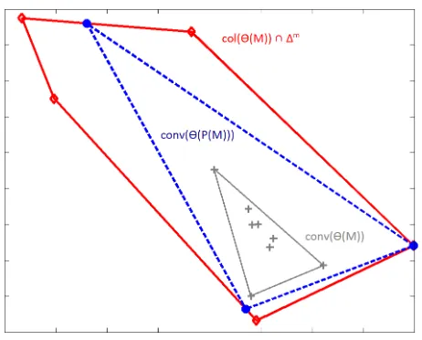
Example 1 Here is an example with a rank-three separable matrix

M=





5 5 5 5 9 1 4 1 7 7

10 6 5 3 7 8 4 1 5 8

8 9 9 4 7 8 3 9 6 7



 T



1 0 0 2 3 6 4 4

0 1 0 5 7 7 7 4

0 0 1 9 4 4 8 6



. (10)

Its (rounded) preprocessed version is given by

P

(M) = 



3.6 3.9 3.9 4.3 7.6 0 3.3 0.5 5.9 5.7

6.3 2.5 1.6 0 1.5 6.5 1.5 0 0.7 3.4

0.8 2.4 2.7 0.7 0.7 1.8 0 4.2 0.9 0.6 

 T

I3 03×5

,

where I3 is the 3-by-3 identity matrix and03_×5 is the 3-by-5 all-zero matrix. Figure 1 shows the

geometric interpretation of the preprocessing.

4.3 Uniqueness and Robustness Through Preprocessing

A potential drawback of the preprocessing is that it might increase the nonnegative rank ofM. In

this section, we show how to modulate the preprocessing to prevent this behavior. Let us define

P

α(M) =M(I₋αB∗) =M₋αMB∗,

where 0_≤α_≤1 and B∗_∈

B

∗(M). Notice that

P

α(M) is well-defined because for any B∗₁,B∗ 2∈

B

∗(M)we haveMB∗₁=MB∗₂; see Theorem 15.

Lemma 26 Let M be a nonnegative matrix such that the vertices ofconv(θ(M))are non-repeated. Then, for any0_≤α_≤β_≤1,

conv(θ(M))_⊆conv(θ(

P

α(M)))_⊆conv(θ(

P

β(M)))_⊆col(θ(M))_∩∆m.

Therefore,

Figure 1: Geometric interpretation of the preprocessing of matrixMfrom Equation (10).

Proof The proof can be obtained by following exactly the same steps as the proof of Lemma 18.

Lemma 27 Let M be a nonnegative matrix such that the vertices ofconv(θ(M))are non-repeated, then the supremum

¯

α= sup 0≤α≤1

α such that rank+(

P

α(M)) =rank+(M) (11)

is attained.

Proof We can assume without loss of generality thatMdoes not have all-zero columns. In fact, if

M:i=0 for someithen

P

α(M):i=0 for allα∈[0,1]so that the nonnegative rank of

P

α(M)is not

affected by the zero columns ofM.

Then, if ¯α=1, the proof is complete. Otherwise, one can easily check that, for any 0_≤α¯ <1, we have

P

α¯(M):i6=0∀i(using a similar argument as in Lemma 17).

Finally, the result follows from the upper-semicontinuity of the nonnegative rank (Bocci et al.,

2011, Theorem 3.1): ‘IfPis a nonnegative matrix, without zero columns and with rank+(P) =k,

then there exists a ball

B

(P,ε) centered at P and of radiusε>0 such that rank+(N)≥k for all

N_∈

B

(P,ε)’. Therefore, if the supremum of (11) was not attained, the matrix

P

α¯(M)would sat-isfy rank+(

P

α¯(M))>rank+(M)while for anyα<α¯ we would have rank+(

P

α(M)) =rank+(M),

a contradiction.

Hence working with matrix

P

α¯(M) instead of M will reduce the number of solutions of the

NMF problem while preserving the nonnegative rank:

exact NMF(U,V Q−1_{)of M, while the converse is not true. In fact,} conv(θ(M))_⊆conv(θ(

P

α¯(M))). Therefore, the NMF problem for

P

α¯(M)is more well posed.

Proof This follows directly from the definition of ¯α, and Lemmas 26 and 27.

We now illustrate Corollary 28 on a simple example, which will lead to three other important results.

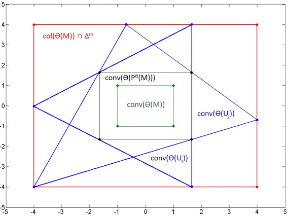
Example 2 (Nested Squares) Let

M=



  

5 3 3 5

3 5 5 3

5 5 3 3

3 3 5 5



  .

The problem NPP(M) restricted to the column space of M is made up of two nested squares,

conv(θ(M))andcol(θ(M))_∩∆m_{, centered at(0,0)with side length 2 and 8 respectively, see}

Fig-ure 2. The polygon corresponding to

P

α(M)is a square centered at(0,0)with side length depend-ing onα, between 2 (forα=0) and 8 (forα=1). We can show that the largest such square still included in a triangle corresponds to

P

α¯(M) =

P

α¯ 

  

5 3 3 5

3 5 5 3

5 5 3 3

3 3 5 5

   = 1 a    

1+a 1₋a 1₋a 1+a

1₋a 1+a 1+a 1₋a

1+a 1+a 1₋a 1₋a

1₋a 1₋a 1+a 1+a



 

, (12)

where a=√2₋1andα¯ =4a_3a−1 (this follows from the proof of Theorem 29; see below). Hence, the polygonconv(θ(

P

α¯(M)))is a square centered at(0,0)with side length8a in betweenconv(θ(M))

andcol(θ(M))_∩∆m_{, see Figure 2. Unfortunately, the exact NMF of}

_P

α¯_{(M)is non-unique. In fact,}

we will see later that it has 8 solutions (the ones drawn on Figure 2 and their rotations).

Example 2 illustrates the following three important facts:

Fact 1. Defining a well-posed NMF problem is not always possible. In other words,there does not exist any ‘reasonable’ NMF formulation having always a unique solution (up to permutation and scaling).In fact, Example 2 shows that, because of the symmetry of the problem, any solution

of NPP(M) can be rotated by 90, 180 or 270 degrees to obtain a different solution with exactly

the same characteristics (the rotated solutions cannot be distinguished in any reasonable way). For example, there are 4 solutions which are the sparsest, each containing one vertex of col(θ(M))_∩∆m_, see conv(θ(U2))on Figure 2, including

U2= 

  

1 a 0

0 1−a 1

a 1 0

1₋a 0 1



 

, andU

(180)

2 =



  

0 1₋a 1

1 a 0

1₋a 1 1

a 0 0



Figure 2: Geometric interpretation of the preprocessing of matrixMfrom Equation (12).

whereU₂(180)is the rotation of 180 degrees ofU2.

Fact 2. The preprocessing makes NMF more robust. For anym-by-nmatrixE such that col(E)_⊆

col(M),M+E_≥0, and

conv(θ(M))_⊆conv(θ(M+E))_⊆conv(

P

α¯(M)),

the exact NMF(U,V) of

P

α¯(M) will still provide an optimal factorU for the perturbed matrix

M+E. In particular, if the matrixM is positive, then one can show that4 conv(θ(M))is strictly contained in conv(

P

α¯(M))(given that ¯α>0) so that any sufficiently small perturbation E with col(E)_⊆col(M)will satisfy the conditions above.

In Example 2, the vertices ofMcan be perturbed and, as long as they remain inside the square

defined by conv(

P

α¯(M)) (see Figure 2), the exact NMF of conv(

P

α¯(M)) will provide an exact

NMF for the perturbed matrix M. (More precisely, any matrix E such that col(E)_⊆col(M)and

maxi,j|Ei j| ≤ √

2₋1 will satisfy conv(θ(M+E))_⊆conv(

P

α¯(M)).)

Fact 3. The preprocessing makes the NMF problem more well-posed. In Example 2, even though

the NMF of

P

α¯(M)is non-unique, the set of solutions has been drastically reduced: from a

two-dimensional space to a zero-two-dimensional one containing eight points: conv(θ(U1)), conv(θ(U2))

and the corresponding rotated solutions, see Figure 2.

Theorem 29 Let M_∈Rm+×n be such that rank(M) =rank+(M) =3 and let α¯ be defined as in

Equation (11). Assume also that conv(θ(

P

(M))) has at least four vertices. Then the number of solutions of NPP(

P

α¯(M)) with three vertices is smaller than m+n.

Proof LetPandQdenote the outer and inner polygons of NPP(

P

α¯(M)), respectively. Let us also

parametrize the boundary of the outer polygonPwith the parametert_∈[0,1]and the function

x:R+→R2:t7→x(t)∈P,

wherexis a continuous function withx(0) =x(1)and_{x(t)_|t∈[0,1]_}is equal to the boundary of

P. We also define the functionxfor values oftlarger than one usingx(t) =x(t_{− ⌊}t_⌋) where_⌊t_⌋is

the largest integer not exceedingt. Using the construction of Aggarwal et al. (1989), we define the

function fk:R+→R+:t7→ fk(t)as follows. Lett1∈[0,1)andx(t1)be the corresponding point

on the boundary of P. Fromx(t1), we can trace the tangent to Q(that is,Qis on one side of the

tangent, and the tangent touchesQ), say in the clock-wise direction, intersect it withPand hence

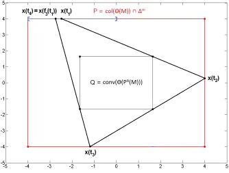
obtain a new pointx(t2) on the boundaryP(see Figure 3 for an illustration on the nested squares problem). We assume without loss of generality thatt2≥t1(ift2happens to be larger than one, we

Figure 3: Mapping of the pointx(t1)tox(t4)using the construction of Aggarwal et al. (1989).

do not round it down with the equivalent valuet2− ⌊t2⌋). Starting fromx(t2), we can use the same procedure to obtain x(t3) and we apply this procedurek times to obtain the pointx(tk+1), where

tk+1≥ ··· ≥t2≥t1. Finally, we define fk(t1) =tk+1.

Aggarwal et al. (1989) showed that x(t1) can be taken as a vertex of a feasible solution of

NPP(

P

α¯(M)) with k vertices if and only if fk(t1) =tk+1 ≥t1+1, that is, we were able to turn around Qinside Pin k+1 steps (in fact, x(t1), x(t2), . . ., andx(tk) are the vertices of a feasible solution).

Aggarwal et al. (1989) also showed that the function fk is continuous, non-decreasing, and

depends continuously on the vertices ofQ(see also Appendix A). Figure 4 displays the function f4

for the nested squares (Example 2).

If col(θ(M))_∩∆m_{has three vertices, then ¯α=1. In fact, we have that}

Figure 4: Function f4(t)for Example 2 using the construction of Aggarwal et al. (1989) (see also Figure 4 and Appendix A). We only plot the function f4in the interval[0,1₈]because, by symmetry, f4(x+1₈) = f4(x) +1₈.

implying rank+(

P

α(M)) =3 for all 0≤α≤1. Moreover, becauseθ(

P

α(M))has at least four

ver-tices, col(θ(M))_∩∆m_{is the unique solution of the corresponding NPP problem: the outer polygon}

is a triangle while the inner polygon has at least four vertices which are located on the edges of the outer triangle (since ¯α=1 and each column of

P

(M)contains at least one zero entry).

Let us then assume that col(θ(M))_∩∆m _{has at least four vertices. We show that this implies}

¯

α<1. Assume ¯α=1. The polygonsP=col(θ(M))_∩∆m_andQ=θ(

_P

_{(M))have at least 4 vertices.}

Moreover, the vertices of Q are located on the boundary of P (because ¯α =1) on at least two

different sides ofP(three vertices cannot be on the same side). It can be shown by inspection that

the optimal solution of this NPP instance must have at least four vertices, hence rank+(

P

(M))>3,

a contradiction.

Next, we show that f4(t)_≤t+1. Assume there existstsuch that f4(t)>t+1. By continuity of f4 with respect to the vertices of Q=conv(θ(

P

α¯(M))), there exists ε>0 sufficiently small such that ¯α+ε<1 and such that the function f₄′ for the NPP instance with inner polygon Q′= conv(θ(

P

α¯+ε(M)))and the same outer polygonPsatisfies f4(t)>t+1 hence rank+(

P

α¯+ε(M))≤3,

a contradiction.

In Appendix A, we prove that fk is made up of pieces which are either constant or strictly

convex, with at mostm+nbreak points corresponding to different solutions to the NPP. Therefore,

because f4is continuous and smaller thant+1, it can intersect the linet+1 only at the break points.

Since there are at mostm+nsuch points corresponding to different NPP solutions, the number of

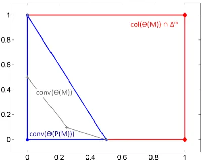
Remark 30 Ifconv(θ(

P

(M)))has three vertices, they define a feasible solution for the correspond-ing NPP problem (that is,

P

(M)is separable, see Theorem 23). However, the number of solutions might be not be finite in that case. Here is an example

M=



  

0 0.5 0.25 0

1 0.5 0.75 1

1 0 0.1 0.5

0 1 0.9 0.5



 

 and

P

(M) = 

  

0 0.5 0 0

1 0.5 0.3 0.5

1 0 0 0

0 1 0.3 0.5



  ,

whose corresponding NPP problems are represented on Figure 5: the NPP of

P

(M)does not have a finite number of solutions.

Figure 5: Counter-example for Theorem 29 when

P

(M)has three vertices.

The fact that the NPP of the matrix

P

α¯(M)can have several different solutions is untypical and, we believe, could be due to the symmetry of the problem (as in Example 2). We conjecture that, in general, the solution to NPP(

P

α¯(M))is unique. In particular, we observed on randomly generated

matrices that it was, see Example 1. In fact, as the function fk(.)defined in Theorem 29 depends

continuously on the inner and outer polytopesQandP, if these polytopes are generated randomly,

there is no reason for the values of the function fk(.)at the break points to be located on the same line as on Figure 4.

We also conjecture that Theorem 29 holds true for any rank:

Conjecture 31 Let M be such that rank(M) =rank+(M) =k and conv(θ(

P

(M))) has at least

(k+1)vertices, andα¯ be defined as in Equation(11), then the number of solutions of NPP(

P

α¯(M)) is finite.

Unfortunately, the geometric construction of Aggarwal et al. (1989) cannot be generalized to three dimensions (or higher). To prove the conjecture, we would need to show that

• Any solution of NPP(

P

α¯(M)) is isolated. Intuitively, the preprocessing

P

α¯(M) ofMgrows the inner polytopeQas long as the corresponding NPP instance has a solution with rank+(M)

vertices. If a solution was not isolated, it could be moved around while remaining feasible,

• The number of isolated solutions is finite. We conjecture that the solutions can be character-ized in terms of the faces ofPandQ, which are finite (depending onmandn).

Remark 32 Of course computingα¯ is non-trivial. However, for matrices of small rank, this could be done effectively. In fact, checking whether the nonnegative rank of an m-by-n is equal torank(M)

can be done in polynomial time in m and n provided that the rank is fixed (Arora et al., 2012). In particular, the algorithm of Aggarwal et al. (1989) does it in

O

((m+n)log(min(m,n)))operations for rank-three matrices (Gillis and Glineur, 2012a). Hence, one could for example use a bisection method to find a good lower boundβ.α¯ and use the corresponding matrix NPP(

P

β(M)) to have a more well-posed NMF problem whose solutions will be solutions of the original one.

5. Preprocessing in Practice

In this section, we address three important practical considerations of the preprocessing.

5.1 Computational Complexity of Solving(8)

It is rather straightforward to check that problem (8) can be decoupled intonindependent CLLS’s,

each corresponding to a different column ofM; for example, for theith column ofM, we have

min b_∈Rn

+

||M:i−Mb||22 such that M:i≥Mb,bi=0. (13)

We then havenCLLS’s withnvariables (actuallyn₋1 since variablebi=0 can be removed) and

m+nconstraints. Using interior point methods, the computational complexity for solving (13) is

of the order of

O

(n3.5); hence the total computational cost is of the order

O

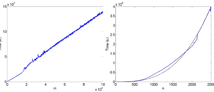
(n4.5).

Figure 6 shows the computational time needed for solving (8) with respect tomfornfixed and

vice versa, for randomly generated matrices (using therand(.)function of MATLABR_{) on a laptop}

3GHz IntelR

CORE i7-2630QM CPU @2GHz 8Go RAM running MATLABR _{R2011b using the}

functionlsqlin(.) of MATLABR_{. The computational time is linear inmwhile being of the order of}

n3 inn, smaller than the expected

O

(n4.5). Therefore, in practice, the dimensionmcan be rather

large while, on a standard machine,ncannot be much larger than 1000. Using parallel architecture

would allow to solve larger scale problems (see also Section 7).

5.2 Normalization of the Columns of

P

(M)

Since the aim eventually is to provide a good approximate NMF to the original data matrixM, we

observed that normalizing the columns of the preprocessed matrix

P

(M)to match the norm of the

corresponding columns ofMgives better results. That is, we replace

P

(M)withD

P

(M)where

Dii= ||

M:i||2 ||

P

(M):i_||2

for alli, and Di j=0 for alli6= j.

This scaling does not change the nice properties of the preprocessing sinceDis a monomial matrix,

henceQDstill is an inverse-positive matrix. This scaling degree of freedom is related to the fact

Figure 6: Computational time for solving (8). On the left, m-by-100 randomly generated

matri-ces; on the right, 1000-by-n randomly generated matrices (plain) and the polynomial

2.6∗10−4n3(dashed).

The reason for this choice is that NMF algorithms are sensitive to the norm of the columns of

M. In fact, when using the Frobenius norm, we have that the following two problems are equivalent

min

U≥0,V≥0||M−UV|| 2

F ≡ _Xmin ≥0,Y≥0

n

∑

i=1 ||M:i||22

M:i ||M:i||2−

XY:i 2 2 .

Therefore, to give each column of

P

(M) the same importance in the objective function as in the

original NMF problem, it makes sense to use the scaling above. This is particularly critical if there

are outliers in the data set: the outliers do not look similar to the other columns of Mhence their

preprocessing will not reduce much theirℓ2-norm (because they are further away from the convex

cone generated by the other columns of M). Therefore, their relative importance in the objective

function will increase in the NMF problem corresponding to

P

(M), which is not desirable.

5.3 Dealing with Noisy Input Matrices and/or Obtaining Sparser Preprocessing

Our technique will typically be useless when the input matrix is noisy and sparse. For example, we have M=   0 0 1 0 1 1 

,

P

(M) =   0 0 1 0 0 1 

 while M_δ=

  0 δ 1 0 1 1 

=

P

(M_δ),

for anyδ>0. This shows that the preprocessing is very sensitive to small positive entries ofM. In order to deal with such noisy and sparse matrices, we propose to relax the nonnegativity constraint

MQ_≥0 in (8), and solve instead

min B∈Rn+×n

n

∑

i=1

M:i−

∑

k₆=i

M:kBki 2

2 such that M:i+ε||M:i||∞e≥_k

∑

6

=i

where 0<ε_≪ 1 and e is the vector of all ones of appropriate dimension. We will denote the corresponding preprocessing

P

ε(M) =M(I−B∗ε)whereB∗ε is an optimal solution of (14). For the

example above withδ=ε=10−2, we obtain

P

ε(Mδ) =





−10−2 10−2

1 ₋10−2

10−4 0.99



.

In practice, this technique also allows to obtain preprocessed matrices with more entries equal or smaller than zero. When choosing the parameterε, it is very important to check whetherρ(B∗_ε)<1 so that the rank of

P

ε(M)is equal to the rank ofMand no information is lost (we can recover the

original matrixM=

P

ε(M)(I−B∗ε)−1given

P

ε(M)andB∗ε).

6. Application to Image Processing

In this section, we apply the preprocessing technique to several image data sets. By construction, the preprocessing procedure will remove from each image a linear combination of the other images. As we will see, this will highlight certain localized parts of these images, essentially because the preprocessed matrices are sparser than the original ones. We will then show that combining the preprocessing with standard NMF algorithms naturally leads to better part-based decompositions, because sparser matrices lead to sparser NMF solutions, see Section 2.

A direct comparison between NMF applied on the original matrix and NMF applied on the preprocessed matrix is not very informative in itself: while the former will feature a lower approx-imation error, the latter will provide a sparser part-based representation. This does not really tell us whether the improvements in the part-based representation and sparsity are worth the increase in approximation error. For that reason, we choose to compare them with a standard sparse NMF tech-nique, described below, in order to better assess whether the increase in sparsity achieved is worth the loss in reconstruction accuracy. Hence, we compare the following three different approaches:

• Nonnegative matrix factorization (NMF). It solves the original NMF problem from Equa-tion (1) using the accelerated HALS algorithm (A-HALS) of Gillis and Glineur (2012b) (with parametersα=0.5 andε=0.1 as suggested by the authors), which is a block coordinate de-scent method.

• Preprocessed NMF for different values of ε. It first computes the preprocessed matrix

P

ε(M) (cf. Section 5.3), then solves the NMF problem for the rescaled preprocessed

ma-trix

P

ε(M)D≈UV′ (cf. Section 5.2) using A-HALS and finally returns(U,V) whereV =

argmin_X≥0||M₋U X_||2_F. This approach will be denoted Pre-NMF(ε). (We will also indicate in brackets the error obtained when usingV=V′Q−1, which will be, by construction, always higher.) Notice that the preprocessed matrix may contain negative entries (whenε>0) which is handled by A-HALS. We do not set these entries to zero for two important reasons: (i) we

want to preserve the column space ofM, (ii) the negative entries ofMlead to sparser NMF

solutions: Geometrically, a negative entry inM means that a vertex of conv(M)(the inner

polytope) is not contained in∆m_{(the outer polytope) making NPP(M) infeasible (as a}

nega-tive entry cannot be obtained with nonneganega-tive ones). However, the approximate solutionT

of NPP(M) will have to be close to the boundary of∆m _{to approximate well that vertex. In}

smaller than_−||max(0,M)_||F then(UV)i j =0 for any optimal solution of NMF (1). There-fore, when indicating the sparsity of the preprocessed matrix, negative entries will be counted as zeros as they lead to even sparser NMF decompositions.

• Sparse NMF. The most standard technique to obtain sparse solutions for NMF problems is to use a sparsity-inducing penalty term in the objective function. In particular, it is well-known

that adding anl1-norm penalty term induces sparser solutions (Kim and Park, 2007), and we

therefore solve the following problem:

min

U,V≥0||M−UV|| 2 F+

r

∑

i=1

µi||U:i||1, ||U:i||∞=1∀i,

where_||x||1=∑i|xi|,||x||∞=maxi|xi|andµiare positive parameters controlling the sparsity

of the columns ofU. In order to solve sNMF, we also use A-HALS which can easily be

adapted to handle this situation. The ℓ∞-norm constraints is not restrictive because of the

degree of freedom in the scaling of the columns ofUand the corresponding rows ofV, while

it prevents matrixU to converge to zero. The theoretical motivation is that thel1-norm is the convex envelope of thel0-norm (that is, the largest convex function smaller than thel0-norm) in theℓ∞-ball, see Recht et al. (2010) and the references therein.

In order to compare sparse NMF with Pre-NMF(ε), the parametersµi 1≤i≤r are tuned in

order to match the sparsity obtained by Pre-NMF(ε). The corresponding approach will be

denoted sNMF(ε).

For each approach, we will keep the best solution obtained among the same ten random

initial-izations (using therand(.)function of MATLABR_{) and each run was allowed 1000 (outer) iterations}

of the A-HALS algorithm. We will use the relative error

100||M−UV||F ||M_||F

to asses the quality of an approximation. We will also display the error obtain by the truncated singular value decomposition (SVD) for the same factorization rank to serve as a comparison. For the sparsity, we use the percentage of non-zero entries5

s(U) =100#zeros(U)

mr ∈ [0,100], forU∈R

m_×r_.

Because the solution computed with Pre-NMF does not directly aim at minimizing the error

||M₋UV_||2_F, it is not completely fair to use this measure for comparison. In fact, it would be

better to compare the quality of the sparsity patterns obtained by the different techniques. For this reason, we use the same post-processing procedure as described by Gillis and Glineur (2010) which benefits all algorithms: once a solution is computed by one of the algorithms, the zero entries of

U are fixed and we minimize minU_≥0,V≥0||M−UV||2F on the remaining (nonzero) entries (again,

A-HALS can easily be adapted to handle this situation and we perform 100 additional steps on each solution), and report the new relative approximation error as “Improved”, while the original relative error before this postprocessing will be reported as “Plain”. The code is available athttps:

//sites.google.com/site/nicolasgillis/code.

6.1 CBCL Data Set

The CBCL face data set6 is made of 2429 gray-level images of faces with 19_×19 pixels (black is

one and white is zero). We look for an approximation of rankr=49 as in Lee and Seung (1999).

Because of the large number of images in the data set, the preprocessing is rather slow. In fact,

we have seen in Section 5.1 that it is in

O

(n4.5) wheren is the number of images in the data set

(it would take about one week on a laptop). Therefore, we only keep every third image for a total of 810 images, which takes less than three hours for the preprocessing; about 10-15 seconds per image.7

Table 1 reports the sparsity and the value ofρ(B∗_ε)for the preprocessed matrices with different values of the parameterε. As explained in Section 5.3, the sparsity of

P

ε(M)increases withε, and

εwas chosen to make sure thatρ(B∗_ε)<1 implying rank(

P

ε(M)) =rank(M).

M

P

(M)

P

0.05(M)

P

0.1(M)

s(.) 0 0.001 20.92 38.03

ρ(B∗_ε) 0 0.71 0.83 0.90

Table 1: CBCL data set: sparsity of the preprocessed matrices

P

ε(M) =MQ and corresponding

spectral radius ofB∗_ε=I₋Q.

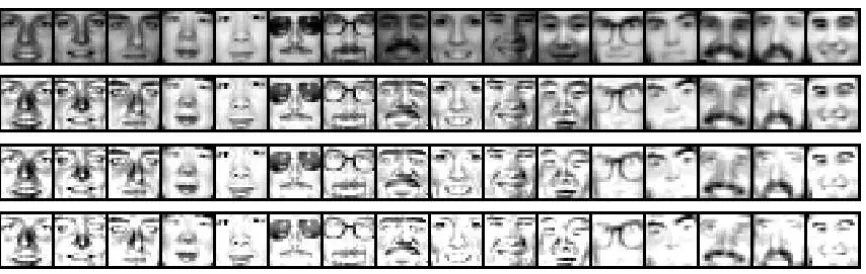
Figure 7 displays a sample of images of the CBCL data set along with the corresponding pre-processed images for different values ofε.

Figure 7: From top to bottom: CBCL sample images, corresponding preprocessed images forε=0,

ε=0.05, andε=0.1.

We observe that the preprocessing is able to highlight some parts of the images: the eyes (faces 5 and 9), the eyebrows (faces 3, 4, 8, 10, 11, 13 and 16), the mustache (faces 14 and 15), the glasses (faces 6, 7 and 12), the nose (faces 1 to 4) or the mouth (faces 1 to 5). Recall that the preprocessing removes from each image of the original data set a linear combination of other images. Therefore,

6. Available athttp://cbcl.mit.edu/software-datasets/FaceData2.html.

7. The MATLABR _{functionlsqlinfor solving CLLS problems is much slower thanquadprogwith interior point (which}