Cumulative Distribution Networks and the Derivative-sum-product
Algorithm: Models and Inference for Cumulative Distribution
Functions on Graphs
Jim C. Huang [email protected]
Microsoft Research One Microsoft Way Redmond, WA 98052, USA
Brendan J. Frey [email protected]
University of Toronto 10 King’s College Rd.
Toronto, ON M5S 3G4, Canada
Editor: Tommi Jaakkola
Abstract
We present a class of graphical models for directly representing the joint cumulative distribution function (CDF) of many random variables, called cumulative distribution networks (CDNs). Un-like graphs for probability density and mass functions, for CDFs the marginal probabilities for any subset of variables are obtained by computing limits of functions in the model, and conditional probabilities correspond to computing mixed derivatives. We will show that the conditional inde-pendence properties in a CDN are distinct from the conditional indeinde-pendence properties of directed, undirected and factor graphs, but include the conditional independence properties of bi-directed graphs. In order to perform inference in such models, we describe the ‘derivative-sum-product’ (DSP) message-passing algorithm in which messages correspond to derivatives of the joint CDF. We will then apply CDNs to the problem of learning to rank players in multiplayer team-based games and suggest several future directions for research.
Keywords: graphical models, cumulative distribution function, message-passing algorithm,
infer-ence
1. Introduction
Probabilistic graphical models provide a pictorial means of specifying a joint probability density function (PDF) defined over many continuous random variables, the joint probability mass function (PMF) of many discrete random variables, or a joint probability distribution defined over a mixture of continuous and discrete variables. Each variable in the model corresponds to a node in a graph and edges between nodes in the graph convey statistical dependence relationships between the variables in the model. The graphical formalism allows one to obtain the independence relationships between random variables in a model by inspecting the corresponding graph, where the separation of nodes in the graph implies a particular conditional independence relationship between the corresponding variables.
neighboring nodes in the graph. Typically, this allows us to decompose a large multivariate dis-tribution into a product of simpler functions, so that the task of inference and estimation of such models can also be simplified and efficient algorithms for performing these tasks can be imple-mented. Often, a complex distribution over observed variables can be constructed using a graphical model with latent variables introduced, where the joint probability over the observed variables is obtained by marginalization over the latent variables. The model with additional latent variables has the advantage of having a more compact factorized form as compared to that for the joint prob-ability over the observed variables. However, this often comes at the cost of a significantly higher computational cost for estimation and inference, as additional latent variables often require one to either approximate intractable marginalization operations (Minka, 2001) or to sample from the model using Markov Chain Monte Carlo (MCMC) methods (Neal, 1993). Furthermore, there is also the problem that there are possibly an infinite number of latent variable models associated with any given model defined over observable variables, so that adding latent variables for any given appli-cation can often present difficulties in terms of model identifiability, which may be desirable when model parameters are to be interpreted. These issues may hamper the applicability of graphical models for many real-world problems in the presence of latent variables.
Another possible limitation of many graphical models is that the joint PDF/PMF itself might not be appropriate as a probability model for certain applications. For example, in learning to rank, the cumulative distribution function (CDF) is a probabilistic representation that arises naturally as a probability of inequality events of the type{X ≤x}. The joint CDF lends itself to such problems that are easily described in terms of inequality events in which statistical dependence relationships also exist among events. An example of this type of problem is that of predicting multiplayer game outcomes with a team structure (Herbrich, Minka and Graepel, 2007). In contrast to the canonical problems of classification or regression, in learning to rank we are required to learn some map-ping from inputs to inter-dependent output variables so that we may wish to model both stochastic orderings between variable states and statistical dependence relationships between variables.
we will use the message-passing algorithm for inference in order to apply CDNs to the problem of learning to rank, where we will show that CDFs arise naturally as a probability models in which it is easy to specify stochastic ordering constraints among variables in the model.
1.1 Notation
Before we proceed, we will establish some notation to be used throughout the paper. We will denote bipartite graphs as
G
= (V,S,E)where V,S are two disjoint sets of nodes and E⊆ {V×S,S×V}is a set of edges that correspond to ordered pairs(α,s)or(s,α)forα∈V and s∈S. We will denote neighboring setsN
(α)andN
(s)asN
(α) ={s∈S :(α,s)∈E},N
(s) ={α∈V :(α,s)∈E}.Furthermore, let
N
(A) =∪α∈AN
(α).Throughout the paper we will use boldface notation to denote vectors and/or matrices. Scalar and vector random variables will be denoted as Xαand XArespectively whereαis a node in a graph
G
and A denotes a set of nodes inG
. The notation|A|,|x|,|X|will denote the cardinality, or number of elements, in set A and vectors x,X respectively. We will also denote the mixed partial deriva-tive/finite difference as∂xAh
·i, where the mixed derivative here is taken with respect to arguments xα∀α∈A. Throughout the paper we assume hat sets consist of unique elements such that for any set A and for any elementα∈A, A∩α=α, so that ∂xA
h
·iconsists of the mixed derivative with
respect to unique variable arguments Xα∈XA. For example,∂x1,2,3
h
F(x1,x2,x3) i
≡ ∂3F
∂x1∂x2∂x3.
1.2 Cumulative Distribution Functions
Here we provide a brief definition for the joint CDF F(x)defined over random variables X, denoted individually as Xα. The joint cumulative distribution function F(x)is then defined as the function F :R|X|7→[0,1]such that
F(x) =P
"
\
Xα∈X
Xα≤xα #
≡P X≤x
.
Thus the CDF is a probability of events{Xα≤xα}. Alternately, the CDF can be defined in terms of the joint probability density function (PDF) or probability mass function (PMF) P(x)via
F(x) = Z x
−∞P
(u)du,
where P(x), if it exists, satisfies P(x)≥0,RxP(x)dx=1 and P(x) =∂x
h
F(x)iwhere∂x
h
·idenotes
the higher-order mixed derivative operator∂x1,···,xK
h
·i≡ ∂ K
∂x1···∂xK
for x= [x1 ··· xK]∈RK.
A function F is a CDF for some probabilityPif and only if F satisfies the following conditions:
1. The CDF F(x)converges to unity as all of its arguments tend to∞, or
F(∞)≡ lim
2. The CDF F(x)converges to 0 as any of its arguments tends to−∞, or
F(−∞,x\xα)≡ lim
xα→−∞F(xα,x\xα) =0 ∀Xα∈X.
3. The CDF F(x)is monotonically non-decreasing, so that
F(x)≤F(y)∀x≤y,x,y∈R|X|.
where x≤y denotes element-wise inequality of all the elements in vectors x,y.
4. The CDF F(x)is right-continuous, so that
lim
ǫ→0+F(x+ǫ)≡F(x)∀x∈R
|X|.
A proof of forward implication in the above can be found in Wasserman (2004) and Papoulis and Pillai (2001).
Proposition 1 Let F(xA,xB)be the joint CDF for variables X where XA,XB for a partition of the
set of variables X. The joint probability of the event{XA≤xA}is then given in terms of F(xA,xB)
as
F(xA)≡P
h
XA≤xA
i
= lim
xB→∞F(xA,xB).
The above proposition follows directly from the definition of a CDF in which
lim
xB→∞F(xA,xB) =P
""
\
α∈A
{Xα≤xα} #
∩
"
\
β∈B
{Xβ≤∞} ##
=P
"
\
α∈A
{Xα≤xα} #
=F(xA).
Thus, marginal CDFs of the form F(xA)can be computed from the joint CDF by computing limits.
1.3 Conditional Cumulative Distribution Functions
In the sequel we will be making use of the concept of a conditional CDF for some subset of variables XAconditioned on event M. We formally define the conditional CDF below.
Definition 2 Let M be an event with P[M]>0. The conditional CDF F(xA|M) conditioned on
event M is defined as
F(xA|M)≡P
h
XA≤xA|M
i
=P
h
{XA≤xA} ∩M
i
PM .
We will now find the above conditional CDF for different types of events M.
Lemma 3 Let F(xC)be a marginal CDF obtained from the joint CDF F(x)as given by Proposition 1 for some XC⊆X. Consider some variable set XA ⊆X where XATXC =/0. Let M=ω(xC)≡
{XC≤xC}for XC⊂X. If F(xC)>0, then F(xA|ω(xC))≡F(xA|XC≤xC) =
F(xA,xC)
F(xC)
Thus a conditional CDF of the form F(xA|ω(xC))can be obtained by taking ratios of joint CDFs,
which consists of computing limits to obtain the required marginal CDFs. It follows from Lemma 3 that marginalization over variables XCcan be viewed as a special case of conditioning on XC<∞.
To compute conditional CDFs of the form F(xA|xβ)where we instead condition on xβ, we need
to differentiate the joint CDF, as we now show.
Lemma 4 Consider some variable set XA⊆X. Let M={xβ<Xβ≤xβ+ε}withε>0 for some
scalar random variable Xβ∈/XA. If F(xβ)and F(xA,xβ)are differentiable with respect to xβso that ∂xβ
h
F(xβ)iand∂xβ
h
F(xA,xβ)
i
exist with ∂xβ
h
F(xβ)i>0, then the conditional CDF F(xA|xβ)≡
lim
ε→0+F(xA|xβ<Xβ<xβ+ε) =εlim→0+ P
h
{XA≤xA} ∩ {xβ<Xβ≤xβ+ε}
i
P
h
xβ<Xβ≤xβ+εi
is given by
F(xA|xβ) = ∂xβ
h
F(xA,xβ)
i
∂xβ
h F(xβ)i
∝ ∂xβ
h
F(xA,xβ)
i
.
Proof We can write
F(xA|xβ<Xβ≤xβ+ε) =P
h
{XA≤xA} ∩ {xβ<Xβ≤xβ+ε}
i
Phxβ<Xβ≤xβ+εi
=
1 εP
h
{XA≤xA} ∩ {xβ<Xβ≤xβ+ε}
i
1 εP
h
xβ<Xβ≤xβ+εi
=
F(xA,xβ+ε)−F(xA,xβ)
ε
F(xβ+ε)−F(xβ)
ε
.
Taking limits, and given differentiability of both F(xβ)and F(xA,xβ)with respect to xβ, the
condi-tional CDF F(xA|xβ)is given by
F(xA|xβ)≡
lim ε→0+
F(xA,xβ+ε)−F(xA,xβ) ε
lim ε→0+
F(xβ+ε)−F(xβ) ε
= ∂xβ
h
F(xA,xβ)
i
∂xβ
h F(xβ)i
∝ ∂xβ
h
F(xA,xβ)
i
,
where the proportionality constant does not depend on xA.
The generalization of the above lemma to conditioning on sets of variables XC⊆X can be found in
the Appendix.
2. Cumulative Distribution Networks
Graphical models allow us to simplify the computations required for obtaining conditional probabil-ities of the form P(xA|xB)or P(xA) by allowing us to model conditional independence constraints
in terms of graph separation constraints. However, for many applications it may be desirable to compute other conditional and marginal probabilities such as probabilities of events of the type
framework for directly modeling the joint cumulative distribution function, or CDF. With the CDN, we can thus expand the set of possible probability queries so that in addition to formulating queries as conditional/marginal probabilities of the form P(xA)and P(xA|xB), we can also compute
proba-bilities of the form F(xA|ω(xB)),F(xA|xB),P(xA|ω(xB))and F(xA), where F(u)≡P
h U≤u
i is a CDF and we denote the inequality event{U≤u}usingω(xU). Examples of this new type of query could be “Given that the drug dose was less than 1 mg, what is the probability of the patient living at least another year?”, or “Given that a person prefers one brand of soda over another, what is the probability of that person preferring one type of chocolate over another?”. A significant advantage with CDNs is that the graphical representation of the joint CDF may naturally allow for queries which would otherwise be difficult, if not intractable, to compute under directed, undirected and factor graphical models for PDFs/PMFs.
Here we provide a formal definition of the CDN and we will show that the conditional indepen-dence properties in such graphical models are distinct from the properties for directed, undirected and factor graphs. We will then show that the conditional independence properties in CDNs include the properties of bi-directed graphs (Drton and Richardson, 2008; Richardson, 2003). Finally, we will show that CDNs provide a tractable means of parameterizing models for learning to rank in which we can construct multivariate CDFs from a product of CDFs defined over subsets of vari-ables.
Definition 5 The cumulative distribution network (CDN) is an undirected bipartite graphical model consisting of a bipartite graph
G
= (V,S,E), where V denotes variable nodes and S denotes factor nodes, with edges in E connecting factor nodes to variable nodes. The CDN also includes a speci-fication of functionsφs(xs)for each function node s∈S, where xs≡xN(s),∪s∈SN
(s) =V and eachfunctionφs:R|N(s)|7→[0,1]satisfies the properties of a CDF. The joint CDF over the variables in
the CDN is then given by the product over CDFsφs:R|N(s)|7→[0,1], or
F(x) =
∏
s∈Sφs(xs),
where each CDFφsis defined over neighboring variable nodes
N
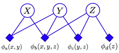
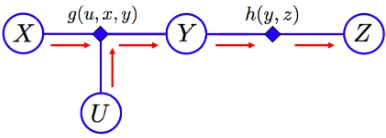
(s).An example of a CDN defined over three variable nodes with four CDN function nodes is shown in Figure 1, where the joint CDF over three variables X,Y,Z is given by
F(x,y,z) =φa(x,y)φb(x,y,z)φc(y,z)φd(z).
In the CDN, each function node (depicted as a diamond) corresponds to one of the functionsφs(xs)
in the model for the joint CDF F(x). Thus, one can think of the CDN as a factor graph for modeling the joint CDF instead of the joint PDF. However, as we will see shortly, this leads to a different set of conditional independence properties as compared to the conditional independence properties of directed, undirected and factor graphs.
Figure 1: A cumulative distribution network (CDN) defined over three variables and four functions.
Lemma 6 If all functions φs(xs) satisfy the properties of a CDF, then the product
∏
s∈S
φs(xs) also
satisfies the properties of a CDF.
Proof If for all s∈S, we have lim
xs→∞φs(xs) =1, then limx→∞
∏
s∈Sφs(xs) =1. Furthermore, if for any givenα∈V and for s∈N
(α), we have limxα→−∞φs(xs) =0, then limxα→−∞
∏
s∈Sφs(xs) =0.To show that the product of monotonically decreasing functions is monotonically non-decreasing, we note that xs<ys for all s∈S if and only if x<y, since∪s∈S
N
(s) =V . Thus ifwe haveφs(xs)≤φs(ys)∀xs<ysfor all s∈S, we can then write
F(x) =
∏
s∈Sφs(xs)≤
∏
s∈Sφs(ys) =F(y).
Finally, a product of right-continuous functions is also right-continuous. Thus if all of the functions
φs(xs)satisfy the properties of a CDF, then the product of such functions also satisfies the properties of a CDF.
Although the condition that each of theφsfunctions be a CDF is sufficient for the overall product
to satisfy the properties of a CDF, we emphasize that it is not a necessary condition, as one could construct a function that satisfies the properties of a CDF from a product of functions that are not CDFs. The sufficient condition above ensures, however, that we can construct CDNs by multiplying together CDFs to obtain another CDF. Furthermore, the above definition and theorem do not assume differentiability of the joint CDF or of the CDN functions: the following proposition shows that differentiability and non-negativity of the derivatives of functionsφswith respect to all neighboring
variables in
N
(s)imply both differentiability and monotonicity of the joint CDF F(x). In the sequel we will assume that whenever CDN functions are differentiable, derivatives are invariant to the order in which they are computed (Schwarz’ Theorem).Proposition 7 If the mixed derivatives∂xA
h
φs(xs)isatisfy ∂xA
h
φs(xs)i≥0 for all s∈S and A⊆
N
(s), then• ∂xC
h
F(x)i≥0 for all C⊆V ,
• F(x)≤F(y)for all x<y,
Proof A product of differentiable functions is differentiable and so F(x)is differentiable. To show that∂xC
h
F(x)i≥0∀C⊆V , we can group the functionsφs(xs)arbitrarily into two functions g(x)
and h(x) so that F(x) =g(x)h(x). The goal here will be to show that if all derivatives∂xA
h g(x)i
and∂xA
h
h(x)iare non-negative, then∂xA
h
F(x)imust also be non-negative. For all C⊆V , applying the product rule to F(x) =g(x)h(x)yields
∂xC
h
F(x)i=
∑
A⊆C∂xA
h
g(x)i∂xC\A
h h(x)i,
so if ∂xA
h
g(x)i,∂xC\A
h
h(x)i≥0 for all A⊆C then ∂xC
h
F(x)i≥0. By recursively applying this
rule to each of the functions g(x),h(x)until we obtain sums over terms involving∂xA
h
φs(xs)
i
∀A⊆
N
(s), we see that if∂xAh
φs(xs)
i
≥0, then∂xC
h
F(x)i≥0∀C⊆V .
Now,∂xC
h
F(x)i≥0 for all C⊆V implies that∂xα
h
F(x)i≥0 for allα∈V . By the Mean Value Theorem for functions of several variables, it then follows that if x<y, then
F(y)−F(x) =
∑
α∈V ∂zα
h
F(z)i(yα−xα)≥0,
and so F(x)is monotonic.
The above ensures differentiability and monotonicity of the joint CDF through constraining the derivatives of each of the CDN functions. We note that although it is merely sufficient for the first-order derivatives to be non-negative in order for F(x)to be monotonic, the condition that the higher-order mixed derivatives∂xC
h
F(x)iof the functionsφs(xs)be negative also implies
non-negativity of the first-order derivatives. Thus in the sequel, whenever we assume differentiability of CDN functions, we will assume that for all s∈S, all mixed derivatives ofφs(xs)with respect to any and all subsets of argument variables are non-negative.
Having described the above conditions on CDN functions, we will now provide some examples of CDNs constructed from a product of CDFs.
Figure 2: A CDN defined over two variables X and Y with functions G1(x,y),G2(x,y).
x
y
2 4 6 8 10 12 2 4 6 8 10 (a) x y
−4 −2 0 2 4 1 2 3 4 5 (b) x y
0 2 4 6 8 0 2 4 6 8 (c)
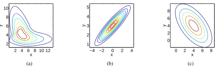
Figure 3: a) Joint probability density function P(x,y) corresponding to the distribution function F(x,y)using bivariate Gaussian CDFs as CDN functions; b),c) The PDFs corresponding
to∂x,y
h
G1(x,y)iand∂x,y
h
G2(x,y)i.
G1(x,y)G2(x,y)with
G1(x,y) =Φ
x y
;µ1,Σ1 !
, µ1=
µx,1 µy,1
, Σ1=
σ2
x,1 ρ1σx,1σy,1
ρ1σx,1σy,1 σ2y,1
,
G2(x,y) =Φ
x y
;µ2,Σ2 !
, µ2=
µx,2 µy,2
, Σ2=
σ2
x,2 ρ2σx,2σy,2
ρ2σx,2σy,2 σ2y,2
,
whereΦ(·; m,S)is the multivariate Gaussian CDF with mean vector m and covariance S. Taking derivatives, the density P(x,y)is given by
P(x,y) =∂x,y
h
F(x,y)i=∂x,y
h
G1(x,y)G2(x,y) i
=G1(x,y)∂x,y
h
G2(x,y)i+∂x
h
G1(x,y)i∂y
h
G2(x,y)i
+∂y
h
G1(x,y) i
∂x
h
G2(x,y) i
+∂x,y
h
G1(x,y) i
G2(x,y).
As functions G1,G2are Gaussian CDFs, the above derivatives can be expressed in terms of Gaus-sian CDF and PDFs. For example,
∂x
h
G1(x,y) i
= Z y
−∞Gaussian
x t
;µ1,Σ1 !
dt
=Gaussian(x; µx,1,σ2x,1)
Z y
−∞Gaussian(t; µy|x,1,σ 2
y|x,1)dt
=Gaussian(x; µx,1,σ2x,1)Φ(y; µy|x,1,σ2y|x,1), where
µy|x,1=µy,1+ρ1
σy,1
σx,1
(x−µx,1),
σ2
Other derivatives can be obtained similarly. The resulting joint PDF P(x,y) obtained by differ-entiating the CDF is shown in Figure 3(a), where the CDN function parameters are given by µx,1=0,µx,2=4,µy,1=3,µy,2=4,σx,1=
√
3,σx,2=
√
5,σy,1=1,σy,2=
√
10,ρ1=0.9,ρ2=−0.6. The PDFs corresponding to∂x,y
h
G1(x,y) i
and∂x,y
h
G2(x,y) i
are shown in Figures 3(b) and 3(c).
The next example provides an illustration of the use of copula functions for constructing multivariate CDFs under the framework of CDNs.
x
y
−3 −2 −1 0 1 −3 −2 −1 0 1 (a) x y
−4 −2 0
−4 −3 −2 −1 0 (b) x y
−2 0 2
−2 −1 0 1 2 (c)
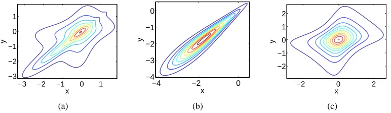
Figure 4: a) Joint probability density function P(x,y) corresponding to the distribution function F(x,y)using bivariate Gumbel copulas as CDN functions, with Student’s-t and Gaussian marginal input CDFs; b),c) The PDFs corresponding to∂x,y
h
G1(x,y) i
and∂x,y
h
G2(x,y) i
.
Example 2 (Product of copulas) We can repeat the above for the case where each CDN function consists of a copula function (Nelsen, 1999). Copula functions provide a flexible means to construct CDN functionsφswhose product yields a joint CDF under Lemma 6. Copula functions allow one
to construct a multivariate CDFφsfrom marginal CDFs{F(xα)}α∈N(s)so that
φs(xs) =ζs
{F(xα)}α∈N(s),
whereζsis a copula defined over variables Xα,α∈
N
(s). For the CDN shown in Figure 2, we canset the CDN functions G1,G2to Gumbel copulas so that
G1(x,y) =ζ1(H1,x(x),H1,y(y)) =exp −
(−log H1,x(x))
1
θ1 + (−log H1,y(y)) 1
θ1
θ1
!
,
G2(x,y) =ζ2(H2,x(x),H2,y(y)) =exp −
(−log H2,x(x))
1
θ2 + (−log H2,y(y)) 1
θ2
θ2
!
,
with H1,x,H2,x set to univariate Gaussian CDFs with parameters µ1,x,µ2,x,σ1,x,σ2,x and H1,y,H2,y
set to univariate Student’s-t CDFs with parametersν1,y,ν2,y. One can then verify that the functions
is shown in Figure 4(a), with the PDFs corresponding to∂x,y
h
G1(x,y)iand∂x,y
h
G2(x,y)ishown in
Figures 4(b) and 4(c).
x
y
−2 0 2 4 6 0
10 20
(a)
x
y
−2 0 2 −20
0 20
(b)
x
y
−10 −5 0 5 −5
0 5
(c)
Figure 5: a) Joint probability density function P(x,y) corresponding to the distribution function F(x,y) using bivariate sigmoidal functions as CDN functions; b),c) The PDFs
corre-sponding to∂x,y
h
G1(x,y)iand∂x,y
h
G2(x,y)i.
Example 3 (Product of bivariate sigmoids) As another example of a probability density function constructed using a CDN, consider the case in which functions G1(x,y)and G1(x,y)in the CDN of Figure 2 are set to be multivariate sigmoids of the form
G1(x,y) = 1
1+exp(−w1
xx) +exp(−w1yy)
,
G2(x,y) =
1 1+exp(−w2
xx) +exp(−w2yy)
,
with w1x,w1y,w2x,w2y non-negative. An example of the resulting joint probability density P(x,y) ob-tained by differentiation of F(x,y) =G1(x,y)G2(x,y)for parameters w1x =12.5,w1y=0.125,w2x=
0.4,w2y = 0.5 is shown in Figure 5(a), with the PDFs corresponding to ∂x,y
h
G1(x,y)i and
∂x,y
h
G2(x,y)ishown in Figures 5(b) and 5(c).
The above examples demonstrate that one can construct multivariate CDFs by taking a product of CDFs defined over subsets of variables in the graph.
2.1 Conditional and Marginal Independence Properties of CDNs
In this section, we will derive the marginal and conditional independence properties for a CDN, which we show to be distinct from those of Bayesian networks, Markov random fields or factor graphs. As with these graphical models, marginal and conditional independence relationships can be gleaned by inspecting whether variables are separated with respect to the graph. In a bipartite graph
G
= (V,S,E), a (undirected) path of length K between two variable nodesα,β∈V consists of a sequence of distinct variable and function nodesα0,s0,α1,s1,···,sK,αKsuch thatα0=α,αK=βα,β∈V\C with respect to
G
if all paths fromα toβ intersect C. Two variable nodesα,β∈V are said to be separated if there exists any non-empty set C that separates them with respect toG
. Similarly, a set C⊆V is said to separate two variable node sets A,B⊆V\C with respect toG
if all paths from any variable nodeα∈A to any variable nodeβ∈B intersect C. Disjoint variable sets A,B∈V are said to be separated if all pairs of nodes(α,β)forα∈A,β∈B are separated.Having defined graph separation for bipartite graphs, we begin with the conditional inequality independence property of CDNs, from which other marginal and conditional independence proper-ties for a CDN will follow.
Theorem 8 (Conditional inequality independence in CDNs) Let
G
= (V,S,E)be a CDN and let A,B⊆V be disjoint sets of variable nodes. If A and B are separated with respect toG
, then for any W⊆V\(A∪B)A⊥⊥B|ω xW
whereω xW
≡ {XW ≤xW}.
Proof If A and B are separated with respect to
G
, then we can writeF(xA,xB,xV\(A∪B)) =g(xA,xV\(A∪B))h(xB,xV\(A∪B))
for some functions g,h that satisfy the conditions of Lemma 6. This means that
F(xA,xB|ω(xW))is given by
F(xA,xB|ω(xW)) =
lim
xV\(A∪B∪W)→∞
F(xA,xB,xV\(A∪B))
lim
xV\W→∞
F(xA,xB,xV\(A∪B))
∝F(xA,xB,xW) =g(xA,xW)h(xB,xW),
which implies A⊥⊥B|ω(xW).
We show that if a CDF F(x) satisfies the conditional independence property of Theorem 8 for a given CDN, then F can be written as a product over functionsφs(xs).
Theorem 9 (Factorization property of a CDN) Let
G
= (V,S,E)be a bipartite graph and let the CDF F(x)satisfy the conditional independence property implied by the CDN described byG
, so that graph separation of A and B by V\(A∪B)with respect toG
implies A⊥⊥B|ω xW
for any W ⊆V\(A∪B) and for any xW ∈R|W|. Then there exist functions φs(xs),s∈S that satisfy the
properties of a CDF such that the joint CDF F(x)factors as
∏
s∈S φs(xs).
Proof The proof here parallels that for the Hammersley-Clifford theorem for undirected graphical models (Lauritzen, 1996). We begin our proof by definingψU(x),ζU(x) as functions that depend
only on variable nodes in some set U⊆V and that form a M¨obius transform pair
ψU(x) =
∑
W⊆UζW(x),
ζU(x) =
∑
W⊆U(−1)|U\W|ψW(x),
where we takeψU(x)≡log F(xU). Now, we note that F(x) can always be written as a product
of functions
∏
U⊆V
of this is to setφV(x) =F(x)andφU(x) =1 for all U⊂V . Since by hypothesis F satisfies all of
the conditional independence properties implied by the CDN described by
G
, if we takeφU(x) =exp ζU(x)
, then it suffices to show that ζU(x)≡0 for subsets of variable nodes U for which
any two non-neighboring variable nodes α,β∈U are separated such that α⊥⊥β|ω(xW) for any
W⊆U\(α,β). Observe that we can writeζU(x)as
ζU(x) =
∑
W⊆U(−1)|U\W|ψW(x)
=
∑
W⊆U\(α∪β)
(−1)|U\W|ψ
W(x)−ψW∪α(x)−ψW∪β(x) +ψW∪α∪β(x)
.
Ifα,β∈U are separated and W ⊆U\(α∪β), thenα⊥⊥β|ω(xW)and
ψW∪α∪β(x)−ψW∪α(x) =log
F(xα,xβ,xW)
F(xα,xW)
=logF(xα|ω(xW))F(xβ|ω(xW))F(xW) F(xα|ω(xW))F(xW)
=logF(xβ|ω(xW))F(xW) F(xW)
=log F(xβ,xW)−log F(xW) =ψW∪β(x)−ψW(x).
Thus if U is any set where nodesα,β∈U are separated, then for all W⊆U\(α∪β)we must have
ψW(x)−ψW∪α(x)−ψW∪β(x) +ψW∪α∪β(x)≡0 and soζU(x) =0. Since F(x) =exp(ψV(x)) =
exp
∑
U ζU(x)
=
∏
U
φU(x)where the product is taken over subsets of variable nodes U that are
not separated. Now, we note that for any U that is not separated, we must have U ⊆
N
(s) (as U =N
(s)∪A for some A withN
(s)∩A=/0implies that U is not separated) for some s∈S and so we can write F(x) =∏
U
φU(x) =
∏
s∈SU⊆∏
N(s)φU(x) =
∏
s∈Sφs(xs), whereφs(xs) =∏U⊆N(s)φU(x)
satisfies the properties of a CDF given that functionsφU(x) each satisfy the properties of a CDF.
Thus we can write F(x) =
∏
s∈Sφs(xs), where each functionφsis defined over the set of variable nodes
N
(s).Thus, if F(x) satisfies the conditional independence property where graph separation of A and B with respect to
G
implies A⊥⊥B|ω(xW)for any W ⊆V\(A,B), then F can be written as a productof functions of the form
∏
s∈S
φs(xs). The above theorem then demonstrates equivalence between the
conditional independence property A⊥⊥B|ω(xW)and the factored form for F(x).
The conditional inequality independence property for CDNs then implies that variables that are separated in the CDN are marginally independent. An example of the marginal independence property for a three-variable CDN in Figure 6, where variables X and Y are separated by variable Z with respect to graph
G
, and so are marginally independent. In a CDN, variables that share no neighbors in the CDN graph are marginally independent: we formalize this with the following theorem.Figure 6: Marginal independence property of CDNs: if two variables X and Y share no common function nodes, they are marginally independent.
Proof Follows from Theorem 8 with xW →∞.
Note that the converse to the above does not generally hold: if disjoint sets A and B do share functions in S, they can still be marginally independent, as one can easily construct a bipartite graph in which variable nodes are not separated in the graph but the function nodes connecting A to B correspond to factorized functions so that A⊥⊥B. Given the above marginal independence property in a CDN, we now consider the conditional independence property of a CDN. To motivate this, we first present a toy example in Figure 7 in which we are given CDNs for variables X,Y,Z,W and we condition on variable Z. Here the separation of X and Y by unobserved variable W implies X ⊥⊥Y|Z, but separation of X and Y by Z only implies the marginal independence relationship X ⊥⊥Y . In general, variable sets that are separated in a CDN by unobserved variables will be conditionally independent given all other variables: thus, as long as two variables are separated by some unobserved variables they are independent, irrespective of the fact that other variables may be observed as well. We formalize this conditional independence property with the following theorem.
Theorem 11 (Conditional independence in CDNs) Let
G
= (V,S,E)be a CDN. For all disjoint sets of A,B,C⊆V , if C separates A from B relative to graphG
thenA⊥⊥B|V\(A∪B∪C).
.
Proof If C separates A from B, then marginalizing out variables in C yields two disjoint subgraphs with variable sets A′,B′, with A⊆A′,B⊆B′, A′∪B′=V\C and
N
(A′)TN
(B′) =/0. From Theorem 10, we therefore have A′⊥⊥B′. Now consider the set V\(A∪B∪C)and let ˜A,B denote a partition˜ of the set so that˜
A∪B˜=V\(A∪B∪C), A˜∩B˜=/0, ˜
A∩B′=/0, B˜∩A′=/0.
From the semi-graphoid axioms (Lauritzen, 1996; Pearl, 1988), A′⊥⊥B′implies A⊥⊥B|V\(A∪B∪ C)since ˜A⊂A′and ˜B⊂B′.
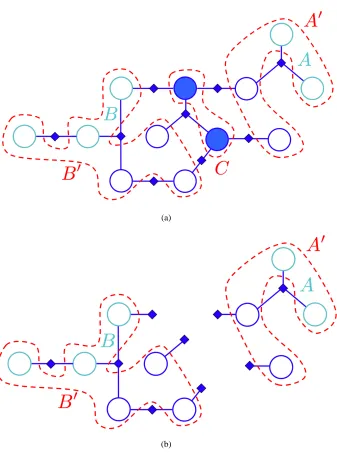
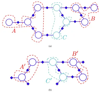
An illustration of the proof is provided in Figures 8(a) and 8(b). The above conditional independence property is distinct from that described in Theorem 8, as in the latter we condition on inequality events of the typeω xW
, whereas in the former we condition on observations xW themselves.
In addition to the above, both the conditional independence properties of Theorem 11 and 8 are closed under marginalization, which consists of computing limits of CDN functions. Thus if
G
is a CDN model for F(x), then the graph for CDN for CDF F(xA) = limxV\A→∞
F(xA,xV\A)is given by
a subgraph of
G
which then implies only a subset of the independence properties ofG
. The next proposition formalizes this.Proposition 12 Let
G
= (V,S,E) be a CDN and let A,B,C⊂V be disjoint sets of nodes with C⊆V\(A∪B)separating A from B with respect toG
. LetG
′= (V′,S′,E′) be a subgraph ofG
with V′⊆V,S′ ⊆S,E′ ⊆E. Similarly, let A′=A∩V′,B′=B∩V′,C′=C∩V′ be disjoint sets of nodes. Then C′separates A′from B′with respect toG
′.The above proposition is illustrated in Figures 9(a) and 9(b). As a result, the conditional indepen-dence relation A′⊥⊥B′|V′\(A′∪B′∪C′)must also hold in the subgraph
G
′, such thatG
′implies a subset of the independence constraints implied byG
. The above closure property under marginal-ization is a property that also holds for Markov random fields, but not for Bayesian networks (see Richardson and Spirtes, 2002 for an example). The above closure and conditional independence properties for CDNs have also been previously shown to hold for bi-directed graphs as well, which we will now describe.2.2 The Relationship Between Cumulative Distribution Networks and Bi-directed Graphs
(a)
(b)
Figure 8: Example of conditional independence due to graph separation in a CDN. a) Given bi-partite graph
G
= (V,S,E), node set C separates set A from B (nodes in light blue) with respect toG
. Furthermore, we have for A′,B′ (nodes in red dotted line) A⊆A′,B⊆B′, A′∪B′=V\C andN
(A′)TN
(B′) =/0as shown. b) Marginalizing out variables corre-sponding to nodes in C yields two disjoint subgraphs ofG
and so A⊥⊥B|V\(A∪B∪C).(a)
(b)
Figure 9: Example of closure under marginalization in a CDN. a) Given CDN
G
= (V,S,E), node set C separates set A from B (nodes in light blue) with respect toG
. b) For subgraphG
′= (V′,S′,E′)with A′⊆A,B′⊆B,C′⊆C, C′separates A′from B′with respect toG
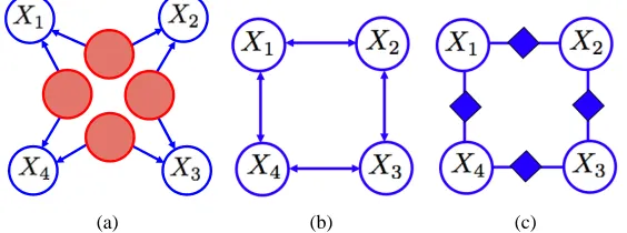
′.a bi-directed graph as(α,β)≡α↔β.1 In a bi-directed graph G, the global Markov property corre-sponds to two disjoint variable sets A,B⊆V satisfying the marginal independence constraint A⊥⊥B if there are no paths between anyα∈A and anyβ∈B. It can be shown (Richardson and Spirtes, 2002) that any bi-directed graphical model corresponds to a directed graphical model with latent variables marginalized out. In particular, we define the canonical directed acyclic graph (DAG) for the bi-directed graph G as a directed graph ˜G with additional latent variables such that ifα↔βin G, thenα←uα,β→βin ˜G for some latent variable uα,β. Thus bi-directed graphical models can be viewed as models obtained from a corresponding canonical DAG with latent variables marginalized out, such that independence constraints between neighboring variable nodes in G can be viewed as arising from the absence of any shared latent variables in the canonical DAG ˜G. This suggests the usefulness of bi-directed graphical models for problems where we cannot discount the presence of unobserved variables but we either A) do not have sufficient domain knowledge to specify distri-butions for latent variables, and/or B) we wish to avoid marginalizing over these latent variables.
In such cases, one can instead attempt to parameterize a probability defined on observed variables using a bi-directed graphical model in which independence constraints among variables are implied by both the corresponding canonical DAG and bi-directed graphs. Examples of a canonical DAG and corresponding bi-directed graph that imply the same set of independence constraints among observed variables are shown in Figures 10(a) and 10(b). Several parameterizations had been pre-viously proposed for bi-directed graphical models. Covariance graphs (Kauermann, 1996) were proposed in which variables are jointly Gaussian with zero pairwise covariance if there is no edge connecting the two variables in the bi-directed graph. In addition, Silva and Ghahramani (2009a) proposed a mixture model with latent variables in which dependent variables in the bi-directed graph can be explained by the causal influence of common components in the mixture model. For bi-directed graphical models defined over binary variables, a parametrization was proposed based on joint probabilities over connected components of the bi-directed graph so that the joint prob-ability of any subset of variables could be obtained by M¨obius inversion (Drton and Richardson, 2008).
Suppose now that we are given a bi-directed graph G and a CDN
G
defined over the samevariables nodes V . Let G and
G
have the same connectivity, such that for any pair of variable nodesα,β∈V , a path betweenα,βexists both in G and
G
. Then both G andG
imply the same set of marginal independence constraints, as we have shown above that in a CDN, two nodes that do not share any function nodes in common are marginally independent (Theorem 10). An example of a bi-directed graph and CDN that imply the same set of marginal independence constraints is shown in Figures 10(b) and 10(c). In addition to implying the same marginal independence constraints as a bi-directed graphical model, the conditional independence property given in Theorem 11 for CDNs corresponds to the dual global Markov property of Kauermann (1996) for bi-directed graphical models, which we now present.Theorem 13 Let G= (V,E)be a bi-directed graphical model and let A,B,C⊆V be three disjoint node sets so that V\(A∪B∪C)separates A from B with respect to G. Then A⊥⊥B|C.
Note that this is identical to the conditional independence property of Theorem 11 where the sepa-rating set is set to V\(A∪B∪C)instead of C.
(a) (b) (c)
While the conditional and marginal independence constraints implied by both a bi-directed graph and a CDN of the same connectivity are identical, Theorem 8 shows that conditional in-dependence constraints of the form A⊥⊥B|ω(xW) are implied in a CDN which are not included
in the definition for a bi-directed graph of the same connectivity. As a result of these additional constraints, CDNs model a subset of the distributions that satisfy the independence constraints of a corresponding bi-directed graph with the same connectivity. In general, CDNs do not model the full set of the probability distributions that can be modeled by bi-directed graphical models with the same connectivity. The following example illustrates how the conditional inequality independence property of CDNs is in general not implied by a bi-directed graphical model with the same graph topology.
Example 4 Consider a 3-variable covariance graph model consisting of the bi-directed graph X1↔X2 ↔X3, where X1,X2,X3 are jointly Gaussian with zero mean and covariance matrixΣ. The proposed covariance graph model imposes the marginal independence constraint X1⊥⊥X3, as there is no edge between variables X1,X3. Denotingσi j as element(i,j) ofΣ, this is equivalent
to the constraintσ13=σ31=0. Now suppose further that the conditional inequality independence property X1⊥⊥X3|ω(x2)is also implied by the covariance graph model. By Theorem 9, this implies that the joint CDF F(x1,x2,x3)factors as
F(x1,x2,x3) =Φ
x1 x2 x3
;0,Σ !
=g(x1,x2)h(x2,x3),
whereΦ(x;µ,Σ)is the multivariate Gaussian CDF with mean zero and covariance matrixΣ, and
g(x1,x2),h(x2,x3) are functions that satisfy the properties of a CDF. The constraints on functions g(x1,x2),h(x2,x3)are given by marginalization with respect to subsets of variables:
F(x1,x2,∞) =g(x1,x2)h(x2,∞),
F(∞,x2,x3) =g(∞,x2)h(x2,x3),
F(∞,x2,∞) =g(∞,x2)h(x2,∞),
so that and so multiplying F(x1,x2,∞)and F(∞,x2,x3), we obtain
F(x1,x2,x3)F(∞,x2,∞) =F(x1,x2,∞)F(∞,x2,x3). (1) Thus, if the conditional inequality independence constraint X1⊥⊥X3|ω(x2)is also implied by the covariance graph model for the joint Gaussian CDF F(x1,x2,x3), then the above equality should hold for all (x1,x2,x3)∈R3 and for any positive-definite covariance matrix Σfor which σ13=
σ31=0. Let x1=x2=x3=0 and letΣbe given by
Σ=
1 √
2
2 0
√ 2
2 1 −
1 2
0 −12 1
,
so thatρ12= √
2
2 ,ρ23=− 1
correlation parameters, so that
F(∞,0,∞) =1
2,
F(0,0,∞) =Φ
0 0
;0,Σ12 !
= 1
4+
1 2πsin
−1ρ 12=
3 8,
F(∞,0,0) =Φ
0 0
;0,Σ23 !
= 1
4+
1 2πsin
−1ρ 23=
1 6,
F(0,0,0) =Φ
0 0 0
;0,Σ !
=1
8+
1 4π(sin
−1ρ
12+sin−1ρ23+sin−1ρ13)
=1
8+
1 4π(sin
−1ρ
12+sin−1ρ23) = 7 48,
whereΣi j is the sub-matrix consisting of rows and columns(i,j)inΣ,ρi j is the correlation
coef-ficient between variables i,j, andρ13=0 is implied by the covariance graph. From Equation (1), we must have
F(0,0,0)F(∞,0,∞) =F(0,0,∞)F(∞,0,0)⇔ 7·1
48·2 = 3·1 8·6,
so that the equality does not hold. Thus, the conditional inequality independence constraint X1⊥⊥ X3|ω(x2) is not implied by the covariance graph model. It can also be verified that the expres-sion for F(x1,x2,x3) given in Equation (1) does not in general correspond to a proper PDF when F(x1,x2),F(x2,x3),F(x2) are Gaussians, as ∂x1,x2,x3
h
F(x1,x2,x3) i
is not non-negative for all
(x1,x2,x3)∈R3.
The previous example shows that while graph separation of variable node sets A,B with respect to both bi-directed graphical models and CDNs of the same connectivity implies the same set of marginal independence constraints, in CDNs we have the additional constraint of A⊥⊥B|ω(xC), a
constraint that is not implied by the corresponding bi-directed graphical model. The above example shows how such additional constraints can then impose constraints on the joint probabilities that can be modeled by CDNs. However, for probabilities that can be modeled by any of CDN, bi-directed graph or corresponding canonical DAG models, CDNs can provide closed-form parameterizations where other types of probability models might not.
In the case of CDNs defined over discrete variables taking values in an ordered set
X
= {r1,···,rK}, the conditional independence property A⊥⊥B|ω(xW)for W ⊆V\(A∪B)(Theorem8) implies that conditioning on the event XC =r11 yields conditional independence between
dis-joint sets A,B,C⊆V in which C separates A,B with respect to
G
. We define the corresponding min-independence property below.Definition 14 (Min-independence) Let XA,XB,XC be sets of ordinal discrete variables that take
on values in the totally ordered alphabet
X
with minimum element r1∈X
defined as r1≺α∀α6= r1,α∈X
. XAand XB are said to be min-independent given XCifXA⊥⊥XB|XC=r11,
Theorem 15 (Min-independence property of CDNs) Let
G
= (V,S,E) be a CDN defined over ordinal discrete variables that take on values in the totally ordered alphabetX
with minimum ele-ment r1∈X
defined as r1≺α∀α6=r1,α∈X
. Let A,B,C⊆V be arbitrary disjoint subsets of V, with C separating A,B with respect toG
. Then XAand XB are min-independent given XC.Proof This follows directly from Theorem 8 with xc=r11.
Thus, in the case of a CDN defined over discrete variables where each variable can have values in the totally ordered alphabet
X
, a finite difference with respect to variables XC, when evaluated atthe vector of minimum elements XC=r11 is equivalent to directly evaluating the CDF at XC=r11.
This means that in the case of models defined over ordinal discrete variables, the particular set of conditional independence relationships amongst variables in the model is determined as a function of the ordering over possible labels for each variable in the model, so that one must exercise care in how such variables are labeled and what ordering is satisfied by such labels.
2.3 Stochastic Orderings in a Cumulative Distribution Network
The CDN, as a graphical model for the joint CDF over many random variables, also allows one to easily specify stochastic ordering constraints between subsets of variables in the model. Informally, a stochastic ordering relationship XY holds between two random variables X,Y if samples of Y tend to be larger than samples of X . We will focus here on first-order stochastic ordering constraints
(Lehmann, 1955; Shaked and Shanthikumar, 1994) of the form X Y and how one can specify
such constraints in terms of the CDN functions in the model. We note that such constraints are not a necessary part of the definition for a CDN or for a multivariate CDF, so that the graph for the CDN alone does not allow one to inspect stochastic ordering constraints based on graph separation of variables. However, the introduction of stochastic ordering constraints, in combination with separation of variables with respect to the graph, do impose constraints on the products of CDN functions, as we will now show. We will define below the concept of first-order stochastic orderings among random variables, as this is the primary definition for a stochastic ordering that we will use. We refer the reader to Lehmann (1955) and Shaked and Shanthikumar (1994) for additional definitions.
Definition 16 Consider two scalar random variables X and Y with marginal CDFs FX(x) and
FY(y). Then X and Y are said to satisfy the first-order stochastic ordering constraint X Y if
FX(t)≥FY(t)for all t∈R.
The above definition of stochastic ordering is stronger than the constraint E[X]≤E[Y]which is often used and one can show that XY implies the former constraint. Note that the converse is not true: E[X]≤E[Y]does not necessarily imply X Y . For example, consider two Gaussian random variables X and Y for which E[X]≤E[Y] but Var[X]≫Var[Y]. The definition of a stochastic ordering can also be extended to disjoint sets of variables XAand XB.
Definition 17 Let XA and XB be disjoint sets of variables so that XA={Xα1,···,XαK}and XB= {Xβ1,···,XβK}for some strictly positive integer K. Let FXA(t)and FXB(t)be the CDFs of XAand
XB. Then XA,XBare said to satisfy the stochastic ordering relationship XAXBif
FXA(t)≥FXB(t)
Having defined stochastic orderings, we will now present the corresponding constraints on CDN functions which are implied by the above definitions.
Proposition 18 Let
G
= (V,S,E) be a CDN, with A,B⊂V so that A={α1,···,αK} and B= {β1,···,βK} for some strictly positive integer K. Let t∈RK. Then A,B satisfy the stochasticordering relationship XAXBif and only if
∏
s∈N(A)
lim
uN(s)\A→∞
φs(uN(s)\A,tN(s)TA)≥
∏
s∈N(B)lim
uN(s)\B→∞
φs(uN(s)\B,tN(s)TB)
for all t∈RK.
The above can be readily obtained by marginalizing over variables in V\A,V\B respectively to obtain expressions for F(xA),F(xB) as products of CDN functions. The corresponding ordering
then holds from Definition 17 if and only if FXA(t)≥FXB(t)for all t∈RK.
2.4 Discussion
We have presented the CDN and sufficient conditions on the functions in the CDN in order for the CDN to model to a CDF. We have shown that the conditional independence relationships that follow from graph separation in CDNs are different from the relationships implied by graph separation in Bayesian networks, Markov random fields and factor graph models. We have shown that the condi-tional independence properties of CDNs include, but are not limited to, the marginal independence properties of bi-directed graphs, such that CDNs model a subset of all probability distributions that could be modeled by bi-directed graphs.
As we have shown, performing marginalization in a CDN consists of computing limits, unlike marginalization in models for probability densities. Furthermore, conditioning on observations in a CDN consists of computing derivatives. In the next section, we show how these two operations can be performed efficiently for tree-structured CDNs using message-passing, where messages being passed in the graph for the CDN correspond to mixed derivatives of the joint CDF with respect to variables in subtrees of the graph.
3. The Derivative-sum-product Algorithm
In the previous section, we showed that for a joint CDF, we could compute conditional probabil-ities of the forms F(xA|ω(xB)),F(xA|xB),P(xA|ω(xB))and P(xA|xB), in addition to probabilities
of the type P(xA),F(xA). In directed, undirected or factor graphs, computing and evaluating such conditional CDFs/PDFs would generally require us to integrate over several variables. In a CDN, computing and evaluating such conditionals corresponds to differentiating the joint CDF and then evaluating the total mixed derivative for any given vector of observations x. In this section we will show that if we model the joint CDF using a CDN with a tree-structured graph, then we can derive a class of message-passing algorithms called derivative-sum-product (DSP) for efficiently computing and evaluating derivatives in CDNs. Since that the CDF factorizes for a CDN, the global mixed derivative can then be decomposed into a series of local mixed derivative computations, where each function s∈S and its derivatives is evaluated for observations xs. Throughout this section, we will