Consistent Distribution-Free
K
-Sample and Independence Tests for
Univariate Random Variables
Ruth Heller [email protected]
Department of Statistics and Operations Research Tel Aviv University
Tel Aviv 69978, Israel
Yair Heller [email protected]
Shachar Kaufman [email protected]
Barak Brill [email protected]
Malka Gorfine [email protected]
Department of Statistics and Operations Research Tel Aviv University
Tel Aviv 69978, Israel
Editor:Kenji Fukumizu
Abstract
A popular approach for testing if two univariate random variables are statistically independent consists of partitioning the sample space into bins, and evaluating a test statistic on the binned data. The partition size matters, and the optimal partition size is data dependent. While for detecting simple relationships coarse partitions may be best, for detecting complex relationships a great gain in power can be achieved by considering finer partitions. We suggest novel consistent distribution-free tests that are based on summation or maximization aggregation of scores over all partitions of a fixed size. We show that our test statistics based on summation can serve as good estimators of the mutual information. Moreover, we suggest regularized tests that aggregate over all partition sizes, and prove those are consistent too. We provide polynomial-time algorithms, which are critical for computing the suggested test statistics efficiently. We show that the power of the regularized tests is excellent compared to existing tests, and almost as powerful as the tests based on the optimal (yet unknown in practice) partition size, in simulations as well as on a real data example.
1. Introduction
Testing if two univariate random variablesXandY are independent of one another, given a random
paired sample(xi, yi)Ni=1, is a fundamental and extensively studied problem in statistics. Classical
methods have focused on testing linear (Pearson’s correlation coefficient) or monotone (Spearman’s
ρ, Kendall’sτ) univariate dependence, and have little power to detect non-monotone relationships.
Recently, there has been great interest in developing methods to capture complex dependencies be-tween pairs of random variables. This interest follows from the recognition that in many modern applications, dependencies of interest may not be of simple forms, and therefore the classical meth-ods cannot capture them. Moreover, in modern applications, thousands of variables are measured simultaneously, thus making it impossible to view the scatter-plots of all the potential pairs of vari-ables of interest. For example, Steuer et al. (2002) searched for pairs of genes that are co-dependent, among thousands of genes measured, using the estimated mutual information as a dependence mea-sure. Reshef et al. (2011) searched for any type of relationship, not just linear or monotone, in large data sets from global health, gene expression, major-league baseball, and the human gut micro-biota. They proposed a novel criterion which generated much interest but has also been criticised for lacking power by Simon and Tibshirani (2011) and Gorfine et al. (2011), and for other theoretical grounds by Kinney and Atwal (2014).
A special important case is when X is categorical. In this case, the problem reduces to that
of testing the equality of distributions, usually referred to as the K-sample problem (where K is
the number of categoriesX can have). Jiang et al. (2014) searched for genes that are differentially
expressed across two conditions (i.e., the 2-sample problem), using a novel test that has higher power over traditional methods such as Kolmogorov–Smirnov tests (Darling, 1957).
For modern applications, where all types of dependency are of interest, a desirable property for a test of independence is consistency against any alternative. A consistent test will have power
increasing to one as the sample size increases, for any type of dependency betweenX andY.
Re-cently, several consistent tests of independence between univariate or multivariate random variables were proposed. Sz´ekely et al. (2007) suggested the distance covariance test statistic, that is the
distance (in weightedL2 norm) of the joint empirical characteristic function from the product of
marginal characteristic functions. Gretton et al. (2008) and Gretton and Gyorfi (2010) considered a family of kernel based methods, and Sejdinovic et al. (2013) elegantly showed that the test of Sz´ekely et al. (2007) is a kernel based test with a particular choice of kernel. Heller et al. (2013)
suggested a permutation test for independence between two random vectorsX andY, which uses
as test statistics the sum over all pairs of points(i, j), i 6= j, of a score that tests for association
between the two binary variablesI{d(xi, X)≤d(xi, xj)}andI{d(yi, Y)≤d(yi, yj)}, whereI(·)
is the indicator function andd(·,·)is a distance metric, on the remainingN−2sample points.
Gret-ton and Gyorfi (2010) also considered dividing the underlying space into partitions that are refined
with increasing sample size. For theK-sample problem, Sz´ekely and Rizzo (2004) suggested the
energy test. This test was also proposed by Baringhaus and Franz (2004) and mentioned in Sejdi-novic et al. (2013) to be related to the maximum mean discrepancy (MMD) test proposed in Gretton et al. (2007) and Gretton et al. (2012a). Harchaoui et al. (2008) adopted the kernel approach of Gretton et al. (2007) and incorporated the covariance into the test statistic by using the kernel Fisher discriminant.
The tests in the previous paragraph are not distribution-free, i.e., the null distribution of the test
tests is typically computed by a permutation test. Another option is to try to estimate the null distri-bution, but this can be very difficult and can lead to over-conservative bounds. For example, Sz´ekely et al. (2007) suggested an asymptotically valid null bound for the significance which they showed was too conservative (see Sejdinovic et al. (2013) for suggestions on how to directly estimate the null distribution). The computational burden of applying the permutation tests to a large family of hypotheses may be great. For example, the yeast gene expression data set from Hughes et al.
(2000) contained N = 300 expression levels for each of6,325Saccharomyces cerevisiaegenes.
In order to test each pair of genes for co-expression, it is necessary to account for multiplicity of
M = 2×10⁷hypotheses. For the permutation tests of Heller et al. (2013) and Sz´ekely et al. (2007),
the number of permutations required for deriving ap-value that is below 0.05/M is therefore of
the order of1010. Since these test statistics are relatively costly to compute for each hypothesis,
e.g.,O(N2)in Sz´ekely et al. (2007), andO(N2logN)in Heller et al. (2013), applying them to the
family ofM = 2×10⁷hypotheses is computationally very challenging, even with sophisticated
re-sampling approaches such as that of Yu et al. (2011). Distribution-free tests have the advantage over non-distribution-free tests, that quantiles of the null distribution of the test statistic can be tabulated once per sample size, and repeating the test on new data for the same sample size will not require recomputing the null distribution. Therefore, the computational cost is only that of computing the test statistic for each of the hypotheses.
We note that for univariate random variables Sz´ekely and Rizzo (2009a) considered using the ranks of each random variable instead of the actual values in the test of distance covariance (Sz´ekely et al., 2007), resulting in a distribution-free test. Similarly, for the test of Heller et al. (2013) replac-ing data with ranks results in a distribution-free test. An earlier work by Feuerverger (1993) defined another test based on the empirical characteristic functions for univariate random variables. The test statistic of Feuerverger (1993) was based on a different distance metric of the joint empirical char-acteristic function from the product of marginal charchar-acteristic functions than that of Sz´ekely et al.
(2007). Moreover, in Feuerverger’s test theX’s andY’s are first replaced by their normal scores,
where the normal scores of theX’s depend on the data only through their ranks among theX’s, and
similarly the normal scores of theY’s depend on the data only through their ranks among theY’s,
thus making this test distribution-free. Pczos et al. (2012) suggested a kernel-based test which uses the MMD after transforming the data to ranks.
A popular approach for developing distribution-free tests of independence considers partitioning the sample space, and evaluating a test statistic on the binned data. A detailed review of distribution-free partition-based tests is provided in Section 1.1 for the independence problem, and in Section
1.2 for theK-sample problem. In 1.3 we describe our goals and the outline of the present paper.
1.1 Review of Distribution-Free Tests of Independence Based on Sample Space Partitions
For detecting any type of dependence betweenX andY, the null hypothesis states thatX andY
are independent,H0 :FXY = FXFY,where the joint distribution of(X, Y)is denoted byFXY,
and the marginal distributions ofXandY, respectively, are denoted byFX andFY. The alternative
is thatXandY are dependent,H1:FXY 6=FXFY.
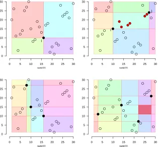
Figure 1 shows example partitions of the sample space based on the ranked observations,
rank(Y) versusrank(X), where am×m partition is based onm−1observations. We refer
Hoeffding (1948b) suggested a test based on summation of a score over all N 2×2DDP of the sample space, which is consistent against any form of dependence if the bivariate density is continuous. Hoeffding’s test statistic is
Z Z
N
n
ˆ
FXY(x, y)−FˆX(x) ˆFY(y)
o2
dFˆXY(x, y),
where Fˆ denotes the empirical cumulative distribution function. Blum et al. (1961) showed that
Hoeffding’s test statistic is asymptotically equivalent toPN
i=1(oi1,1oi2,2−oi1,2oi2,1)2/N4,whereoiu,v,
u, v ∈ {1,2}, is the observed count of cell (u, v) in the 2×2contingency table defined by the
ith observation. Thas and Ottoy (2004) noted that by appropriately normalizing each term in the
sum, the test statistic becomes the average of all Pearson statistics for independence applied to
the contingency tables that are induced by2×2sample space partitions centered about observation
i∈ {1, . . . , N}. They proved that the weighted version of Hoeffding’s test statistic is still consistent.
Partitioning the sample space into finer partitions than the2×2quadrants of the classical tests,
based on the observations, was also considered in Thas and Ottoy (2004). They suggested that the
average of all Pearson statistics on finer partitions of fixed size m×m may improve the power,
but did not provide a proof that the resulting tests are consistent. They examined in simulations
only3×3and4×4partitions. Reshef et al. (2011) suggested the maximal information coefficient,
which is a test statistic based on the maximum over dependence scores taken for partitions of various sizes, after normalization by the partition size, where the purpose of the normalization is equitability rather than power. Since computing the statistic exactly is often infeasible, they resort to a heuristic for selecting which partitions to include. Thus, in practice, their algorithm goes over only a small fraction of the partitions they set out to examine. In Section 4 we show that the power of this test is typically low.
1.2 Review of theK-Sample Problem
As in Section 1.1, we focus on consistent partition-based distribution-free tests. For testing equality
of distributions, i.e., for a categoricalX, one of the earliest and still very popular distribution-free
consistent tests is the Kolmogorov–Smirnov test (Darling, 1957), which is based on the maximum
score of all N partitions of the sample space based on an observed data point. Aggregation by
summation over allN partitions has been considered by Cramer and von Mises (Darling, 1957),
Pettitt (Pettitt, 1976) who constructed a test-statistic of the Anderson and Darling family (Anderson and Darling, 1952), and Scholz and Stephens (1987).
Thas and Ottoy (2007) suggested the following extension of the Anderson–Darling type test. For
random samples of sizeN1andN−N1, respectively, from two continuous densities, for a fixedm,
they consider all possible partitions intomintervals of the sample space of the univariate continuous
random variable. They compute Pearson’s chi-square score for the observed versus expected (under the null hypothesis that the two samples come from the same distribution) counts, then aggregate by summation to get their test statistics. A permutation test is applied on the resulting test statistic,
since under the null all NN
1
assignments of the group labels are equally likely. They show that the
suggested statistic form = 2 is the Anderson–Darling test. They examined in simulations only
partitions intom≤4intervals.
0 5 10 15 20 25 30 0
5 10 15 20 25 30
rank(X)
rank(Y)
i
0 5 10 15 20 25 30
0 5 10 15 20 25 30
rank(X)
rank(Y) i
j
0 5 10 15 20 25 30
0 5 10 15 20 25 30
rank(X)
rank(Y)
0 5 10 15 20 25 30
0 5 10 15 20 25 30
rank(X)
rank(Y)
Figure 1: A visualization of the partitioning of the rank–rank plane which is at the basis of the data
derived partitions (DDP) tests. Here,N = 30, and circles represent observed points. Full
black circles represent those observations that were chosen to induce the partition, and
different shades represent partition cells. Withm= 2, all cells are corner cells (top-left);
withm= 3, the center cell has two vertices which are observed sample points (top-right);
withm = 4, all internal cells, i.e., cells that are not on the boundary, have at least one
observed point vertex (bottom-left); only withm ≥ 5, there exists at least one internal
They developed an efficient dynamic programming algorithm to determine the optimal partition,
and suggested a distribution-free permutation test to compute thep-value.
Although there are many additional tests for the two-sample problem, the list above contains the most common as well as the most recent developments in this field. Interestingly, when working with ranks, the energy test of Sz´ekely and Rizzo (2004) and the Cramer–von Mises test turn out to be equivalent.
1.3 Overview of This Paper
In this work, we suggest several novel distribution-free tests that are based on sample space parti-tions. The novelty of our approach lies in the fact that we consider aggregation of scores over all
partitions of sizem×m(or m for theK-sample case), wherem can increase with sample size
N, as well as consideration of allms simultaneously without any assumptions on the underlying
distributions. In Section 2 we present the new tests both for the independence problem and for
the K-sample problem, with a focus on our regularized scores (that consider all ms) in Section
2.1. We prove that all suggested tests are consistent, including those presented in Thas and Ot-toy (2004), and show the connection between our tests and mutual information (MI). In Section 3
we present innovative algorithms for the computation of the tests, which are essential for largem
since the computational complexity of the naive algorithm is exponential in m. Simulations are
presented in Section 4. Specifically, in Section 4.1 we show that for the two-sample problem for complex distributions there is a clear advantage for fine partitions, while for simple distributions rougher partitions have an advantage. In Section 4.2 we show that, for the independence prob-lem, typically finer partitions have a clear advantage for complex non-monotone relationships. On the other hand, for simpler relationships, there is an advantage for rougher partitions. We further demonstrate the ability of our regularized method (which aggregates over all partitions) to adapt and find the best partition size. Moreover, in simulations we show that for complex relationships all these tests are more powerful than other existing distribution-free tests. In Section 5 we analyze the yeast gene expression data set from Hughes et al. (2000). With our distribution-free tests, we discover interesting non-linear relationships in this data set that could not have been detected by the classical tests, contrary to the conclusion in Steuer et al. (2002) that there are no non-monotone associations. Efficient implementations of all statistics and tests described herein are available in the
R packageHHG, which can be freely downloaded from the ComprehensiveR Archive Network,
http://cran.r-project.org/. Null tables can be downloaded from the first author’s web site.
2. The Proposed Statistics
We assume thatY is a continuous random variable, and thatXis either continuous or discrete. We
haveNindependent realizations(x1, y1), . . . ,(xN, yN)from the joint distribution ofXandY. Our
test statistics will only depend on the marginal ranks, and therefore are distribution free, i.e., their
null distributions are free of the marginal distributionsFX andFY.
Test statistics for theK-sample problem We first consider the case thatX is categorical with
K ≥ 2categories. In this case, a test of association is also aK-sample test of equality of
distri-butions. ForN observations, there are N2+1possible cells, and Nm−−11 possible partitions of the
observations is the same regardless of whether the partition is defined on the original observations or on the ranked observations, and the statistics we suggest only depend on these cell
member-ships, we describe the proposed test statistics on the ranked observations,rank(Y) ∈ {1, ..., N}.
LetΠm denote the set of partitions into m cells. For any fixed partitionI = {i1, . . . , im−1} ⊂
{1.5, . . . , N −0.5}, i1 < i2 < . . . < im−1, C(I) is the set ofm cells defined by the partition.
For a cell C ∈ C(I), let oC(g) and eC(g) be the observed and expected counts inside the cell
for distribution g ∈ {1, . . . , K}, respectively. The expected count eC(g) is the width of cellC
based on ranks multiplied byNg/N, whereNg is the total number observations from distribution
g:e[il,il+1](g) = (il+1−il)×Ng/N, wherel∈ {0, . . . , m−1},i0 = 0.5andim =N + 0.5. We
consider either Pearson’s score or the likelihood ratio score for a given cellC,
tC ∈
K
X
g=1
[oC(g)−eC(g)]2
eC(g)
,
K
X
g=1
oC(g) log
oC(g)
eC(g)
. (1)
For a given partitionI, the score isTI =P
C∈C(I)tC (where iftC =PKg=1oC(g) logoeCC((gg)) then
TI is the likelihood ratio given the partition). Our test statistics aggregate over all partitions by
summation (Cramer–von Mises-type statistics) and by maximization (Kolmogorov–Smirnov-type statistics):
Sm=
X
I∈Πm
TI, Mm= max
I∈Πm
TI. (2)
Tables of critical values for given sample sizes N1, . . . , NK can be obtained for (very) small
sample sizes by generating all possible N!/(ΠKg=1Ng!)reassignments of ranks {1, . . . , N} toK
groups of sizesN1, . . . , NK and computing the test statistic for each reassignment. Thep-value is
the fraction of reassignments for which the computed test statistics are at least as large as observed. When the number of possible reassignments is large, the null tables are obtained by large scale
Monte Carlo simulations (we usedB= 106replicates for each given sample sizeN
1, . . . , NK). For
each of theBreassignments selected at random from all possible reassignments, the test statistic is
computed. Clearly, theB computations do not depend on the data, hence the tests based on these
statistics are distribution free. Again, the p-value is the fraction of reassignments for which the
computed test statistics are at least as large as the one observed, but here the fraction is computed
out of the B + 1assignments that include the B reassignments selected at random and the one
observed assignment, see Chapter 15 in Lehmann and Romano (2005). The test based on each of these statistics is consistent:
Theorem 1 LetY be continuous, andXcategorical withKcategories. LetNgbe the total number
of observations from distribution g ∈ {1, . . . , K}, and N = PK
g=1Ng. If the distribution of Y
differs at a continuous density point y0 across values ofX in at least two categories, label these 1 and 2,limN→∞ min(NN1,N2) > 0, andm finite orlimN→∞m/N = 0, then the distribution-free permutation tests based onSmandMmare consistent.
We omit the proof, since it is similar to (yet simpler than) the proof of Theorem 2 below.
Test statistics for the independence problem We now consider the case that X is continuous.
ForN pairs of observations, there are Nm−−11× Nm−−11
cells, where a cell is a rectangular area in the plane. We refer to these partitions as the all derived
partitions (ADP) and denote this set by ΠADPm . Since the cell membership of observations is the
same regardless of whether the partition is defined on the original observations or on the ranked observations, and the statistics we suggest only depend on these cell memberships, we describe the
proposed test statistics on the ranked observations, so theN pairs of observations are on the grid
{1, . . . , N}2. For any fixed partitionI = {(i
1, j1), . . . ,(im−1, jm−1)} ⊂ {1.5, . . . , N −0.5}2,
, i1 < i2 < . . . < im−1, j1 < j2 < . . . < jm−1, C(I) is the set of m×m cells defined by
the partition. For a cell C ∈ C(I), let oC and eC be the observed and expected counts inside
the cell, respectively. The expected count in cellCwith boundaries[ik, ik+1]×[jl, jl+1]iseC =
(ik+1−ik)×(jl+1−jl)/N, wherek, l ∈ {0, . . . , m−1},i0 =j0 = 0.5, im =jm =N + 0.5.
As with theK-sample problem, we consider either Pearson’s score or the likelihood ratio score for
a given cellC,
tC ∈
(oC−eC)2
eC
, oClog
oC
eC
. (3)
For a given partition I, the score is TI = P
C∈C(I)tC (where if tC = oClog
oC
eC then T
I is
the likelihood ratio given the partition). As above, we consider as test statistics aggregation by summation and by maximization:
SmADP×m=
X
I∈ΠADP
m
TI, MmADP×m= max
I∈ΠADP
m
TI. (4)
We consider another test statistic based on DDP, where each set ofm−1observed points in their
turn define a partition (see Figure 1). This variant has a computational advantage over the ADP
statistic form <5, see Remark 3.1. Since all observations have unique values, the remainingN−
(m−1)points are inside cells defined by the partition. There are mN−1partitions, denote this set of
partitions byΠDDPm . As before, since the cell membership of observations is the same regardless of
whether the partition is defined on the original observations or on the ranked observations, and the statistics we suggest only depend on these cell memberships, we describe the proposed test statistics
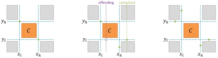
on the ranked observations. For a cellC ∈ C(I), whereI ∈ ΠDDPm , the boundaries ofCare not
necessarily defined by two sample points, as depicted at the bottom right panel of Figure 1. We
refer to rl andrh as the lower and upper values of the ranks ofX inC, and tosl andsh as the
lower and upper values of the ranks ofY inC, whererl, rh, sl, sh ∈ {1, . . . , N}. LetoC andeC be
the observed and expected counts strictly inside the cell, respectively. The expected count in cellC
with rank range[rl, rh]×[sl, sh]iseC = (rh−rl−1)(sh−sl−1)/[N−(m−1)]. We consider
Pearson’s score or the likelihood ratio score for a given cellC, and definetC as in (3). For a given
partitionI, the score isTI =P
C∈C(I)tC, and similarly to (4) we define
SmDDP×m =
X
I∈ΠDDP
m
TI, MmDDP×m = max
I∈ΠDDP
m
TI. (5)
For each of the test statistics in (4) and (5), tables of exact critical values for a given sample
size N can be obtained for small N by generating all possible N!permutations of {1, . . . , N}.
For each permutation (π(1), . . . , π(N)), the test statistic is computed for the reassigned pairs
(1, π(1)), . . . ,(N, π(N)). Clearly, the computation of these null distributions does not depend
on the data, hence the tests based on these statistics are distribution free. As in the case of theK
are at least as large as the one observed, and when the number of possible permutations is large, the critical values are obtained by large scale Monte Carlo simulations. The test based on each of these statistics is consistent:
Theorem 2 Let the joint density ofX andY beh(x, y), with marginal densitiesf(x)andg(y). If there exists a point(x0, y0) such thath(x0, y0)is continuous andh(x0, y0) 6= f(x0)g(y0), i.e.,
there is local dependence at a continuous density point, and ifmis finite orlimN→∞m/
√ N = 0, then the distribution-free permutation tests based on the following test statistics are consistent:
1. The test statistics aggregated by summation: SmDDP×mandSADPm×m.
2. The test statistics aggregated by maximization:MmDDP×m andMmADP×m.
A proof is given in Appendix A. For finitem, asN → ∞, our test statistics converge to population
measures of deviation from independence that are zero if and only if the independence hypothesis
is true (see Hoeffding (1948a) for a discussion of a similar population quantity whenm= 2). For
mgrowing withN, our test statistics estimate the mutual information, as detailed below.
We note that Thas and Ottoy suggestedSm withtC =P2g=1 (oC(g)−eC(g))
2
eC(g) in Thas and Ottoy
(2007), and SmDDP×m using Pearson’s score for finite m in Thas and Ottoy (2004). However, they
examined in simulations onlym ≤ 4. Thanks to the efficient algorithms we developed, detailed
in Section 3, we are able to test for anym ≤ N in the K-sample problem, and for aggregation
by summation in the test of independence. If the aggregation is by maximization in the test of
independence, the algorithm, detailed in Section 3, is exponential inmand thus the computations
are feasible only form≤4.
We shall show in Section 4 that the power of the test based on a summation statistic can be different from the power of the test based on a maximization statistic, and which is more powerful
depends on the joint distribution. However, for both aggregation methods, usingm >3partitions
improves power considerably for complex settings. Therefore, in complex settings our tests with
m > 3have a power advantage over the classical distribution-free tests, which focused on rough
partitions, typicallym= 2.
Connection to the MI An attractive feature of the statisticsSmandSADPm×m, formlarge enough,
is that they are directly associated with the MI (IXY =
R
h(x, y) log[h(x, y)/{f(x)g(y)}]dxdyfor
continuousXandY). MI is a useful measure of statistical dependence. The variablesXandY are
independent if and only if the MI is zero. Estimated MI is used in many applications to quantify the relationships between variables, see Steuer et al. (2002), Paninski (2003), Kinney and Atwal (2014) and references within. Although many works on MI estimation exist, no single one has been accepted as a state-of-the-art solution in all situations (Kinney and Atwal, 2014). A popular
estimator among practitioners due to its simplicity and consistency is thehistogramestimator, where
the data are binned according to some scheme and the empirical mutual information of the resulting partition, i.e, the likelihood ratio score, is computed. Intuitively, one can expect that the statistic
SmADP×m, properly normalized, can also serve as a consistent estimator of the mutual information,
when the contingency tables are summarized by the likelihood ratio statistic, since it is the average of histogram estimators, over all partitions. This intuition is true despite the fact that the number of partitions goes to infinity, since we show that the convergence is uniform and that the fraction of
“bad” partitions (i.e., partitions with cells that are too big or too small) is small, as long asmgoes
Theorem 3 SupposeXis categorical withK categories andY is continuous. LetNg be the total
number of observations from distributiong∈ {1, . . . , K}, andN =PK
g=1Ng. IflimN→∞ NNg >0 forg = 1, . . . , K,limN→∞ mN = 0, andlimN→∞m =∞, then Sm
N(N−1 m−1)
is a consistent estimator
of the MI.
Theorem 4 Suppose the bivariate density of(X, Y)is continuous with bounded mutual informa-tion. IflimN→∞m/
√
N = 0, andlimN→∞m=∞, then
SADP m×m
N(N−1 m−1)×(
N−1 m−1)
is a consistent estimator
of the MI.
See Appendix B for a proof of Theorem 4. The proof of Theorem 3 is omitted since it is similar to
that of Theorem 4. See Appendix D for a simulated example of MI estimation usingSmDDP×m,SmADP×m,
and the histogram estimator. The ADP estimator is the least variable, as is intuitively expected since it is the average over many partitions.
Remark 2.1 In this work we assume there are no ties among the continuous variables. In our software, tied data are broken randomly, so that our test remains distribution free. An alternative approach, which is no longer distribution free, is a permutation test on the ranks, with average ranks for ties. Then a tied observation, that falls on the border of a contingency table cell, receives equal weight in each of the cells it borders with.
2.1 The Proposed Regularized Statistics
An important parameter of the statistics proposed above ism, the partition size. A poor choice of
mmay lead to substantial power loss: ifmis too small or too large, it may lack power to discover
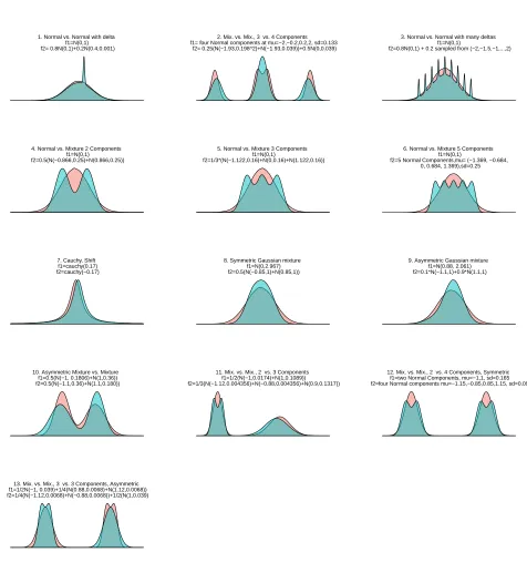
complex non-monotone relationships. For example, consider the three simulation settings for the two-sample problem in the first row of Figure 2. The best partition for setting 1, “normal vs. normal with delta”, for small sample sizes, is intuitively to divide the real line into three cells: until the start of the narrow peak, the support of the narrow peak, and after the peak ends. Moreover, the best aggregation method is by maximization, not summation, since there are very few good partitions
that capture the peak and aggregation by summation usingm= 3will aggregate many bad partitions
that miss the peak. Therefore, we expect thatM3will be the most powerful test statistic for setting
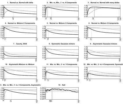
1. For setting 2, “Mix. vs. Mix. 3 vs. 4 components”, intuitively it seems best to partition into more than seven cells, and that many partitions will work well. For setting 3, “normal vs. normal with many deltas”, it seems best to partition into many cells. Indeed, the power curves in Figure 3
show that for the first setting,Mmis optimal at valuem= 3, yet if we use this value for the second
setting, the test has 20% lower power than optimal power (which is 86% atm = 10), and if we
use this value for the third setting, the test has 58% less power than the optimal power (which is
88% atm = 34). Since the optimal choice of mis unknown in practice, we suggest two types of
regularizations which take into consideration the scores from all partition sizes.
The combinedp-values statistic The first type of regularization we suggest is to combine thep
-values from eachm, so that the test statistic becomes the combinedp-value. Specifically, letpm be
thep-value from a test statistic based on partition sizem, be itSmorMmfor theK-sample problem,
orSmADP×m orSmDDP×m for the independence problem. Due to the computational complexity, we do
minm∈{2,...,mmax}pm, as well as the Fisher combinedp-value,−
Pmmax
m=2 logpm. These combined
p-values are notp-values in themselves, but their null distribution can be easily obtained from the
null distributions of the test statistics for fixed ms, as follows: (1) for each of B permutations,
compute the test statistics for each m ∈ {2, . . . , mmax}; (2) compute the p-value of each of the
resulting statistics, so for each permutation, we have a set ofp-valuesp2, . . . , pmmaxto combine; (3)
combine thep-values for each of theBpermutations. ChooseBto be large enough for the desired
accuracy of approximation of the quantiles of the null distribution of the combinedp-values used
for testing. Obviously, since the combinedp-values are based on the ranks of the data, they are
distribution-free. Since they do not require fixingmin advance, they are a practical alternative to
the tests that requiremas input.
In order to examine how close this regularized score is to the optimalm(i.e., themwith highest
power), we looked at the distribution of the ms with minimum p-values in 20,000 data samples
from the above-mentioned three simulation settings. For these settings, using the aggregation by
maximization statistic, the medianm of the minimalp-value was: 3 for the first setting, 9 for the
second setting, and 33 for the third setting. Moreover, the first and third quartiles were 3 to 5 for the first setting, 7 to 14 for the second setting, and 19 to 60 for the third setting. We conclude that
for these examples, themthat achieves the minimump-values in most runs was remarkably close
to the optimalm(which was 3, 10, and 34 for settings 1,2, and 3, respectively), suggesting that the
power of the minimump-value statistic is close to that of the statistic with optimalm. Indeed, the
power of the minimump-values in settings 1-3 using aggregation by maximum was 0.825, 0.799,
and 0.785, whereas the power using the (unknown in practice) optimalmin settings 1-3 was 0.894,
0.86, and 0.88, respectively. Further empirical investigations detailed in Section 4 give additional support to this regularization method.
An extensive numerical investigation, partially summarized in Appendix G, led us to choose the
minimump-value as the preferred regularization method. Between the two combining functions, we
preferred the minimum over Fisher, since Fisher was far more sensitive to the choice of the range of
mfor combining (see Table 6). This regularized statistic is consistent, as the next theorems show.
Theorem 5 Let Y be continuous, and X categorical. Let Ng be the total number of
observa-tions from distributiong ∈ {1, . . . , K}, andN = PK
g=1Ng. If the distribution of Y differs at
a continuous density point y0 across values of X in at least two categories, label these 1 and 2,
limN→∞ min(NN1,N2) > 0, then the permutation test based on minm∈{2,...,mmax}pm is consistent, if:
1. it is based onSm, m∈ {2, . . . , mmax}, andlimN→∞mmax/
√
N = 0ormmaxis finite.
2. it is based onMm, m∈ {2, . . . , mmax}andlimN→∞mmax/N = 0ormmaxis finite.
Theorem 6 Let the joint density ofX andY beh(x, y), with marginal densitiesf(x)andg(y). If there exists a point (x0, y0) such that h(x0, y0) is continuous and h(x0, y0) 6= f(x0)g(y0), i.e., there is local dependence at a continuous density point, then the permutation test based on
minm∈{2,...,mmax}pmis consistent, if
1. it is based onSmDDP×morSmADP×m, andlimN→∞mmax/N1/3 = 0ormmaxis finite.
2. it is based onMmDDP×m andMmADP×m, andlimN→∞mmax/
√
The proof of Theorem 6 follows in a straightforward way from the proofs of Theorem 2, see Ap-pendix C for details. The proof of Theorem 5 follows similarly from the proof of Theorem 1, and it is omitted.
The penalized statistic The test statistic is the maximum (over allms) of the statistic plus penalty.
For theK-sample problem, Jiang et al. (2014) suggested assigning a prior on the partition scheme
and they regularized the likelihood ratio score using this prior. Specifically, they assumed the
par-tition size is Poisson and the conditional distribution on thempartition widths (normalized to sum
to one) isDirichlet(1, . . . ,1). This led to their penalty term−λ0(logN)(m−1), whereλ0 >0
has to be fixed. We assume that the marginal distribution on the partition size isπ(m)(e.g., Poisson
or Binomial), and that the prior probability of selectingI givenm,π(I|m), is uniform. There is
an important difference between our uniform discrete prior distribution on partitions of sizemand
the continuous Dirichlet uniform prior of Jiang et al. (2014). Our prior is uniform on all partitions
that truly divide the sample space intomcells, i.e., we cannot have two partition lines between two
consecutive samples, since this is actually anm−1partition. Using the continuous Dirichlet prior
results in practice in at most mpartitions, but the partition size may also be strictly smaller than
m if two partition points lie between two sample points. Therefore, their conditional distribution
given the partition size parameter is not necessarily the true size of the partition. Their penalty
translates to a conditional probability given a true partition sizemof (N(−m1)−(m1)!−1), compared to our
π(I|m) = 1/ Nm−−11
. Therefore, their score penalizes more severely largems, and their regularized
test statistic has less power when the optimalmis large in our simulations.
For aggregation by maximum in theK-sample problem, we consider the regularized statistic,
max m∈{2,...,mmax}
{Mm+ log[π(I|m)π(m)]}, (6)
where we use the likelihood ratio score per partition. Due to the computational complexity, we do
not consider a regularized score forMm×m. For aggregation by summation, our efficient algorithms
described in Section 3 enable us to consider the penalized average score perm,
max m∈{2,...,mmax}
{SLRmπ(I|m) + logπ(m)} (7)
whereSLRmπ(I|m)isSmdivided by the number of partitions of sizemfor theK-sample test, and
SmADP×m(orSmDDP×m) divided by the number of partitions of sizem×mfor the test of independence,
using the likelihood ratio score per partition. The null distribution of these regularized statistics is computed by a permutation test, and they are distribution free.
Regularization using priors was less effective than using combinedp-values, except when the
Poisson prior was used with parameter λ = √N (see Table 7). We preferred the first type of
regularization since it was at least as effective as regularizing by a Poisson prior, without requiring setting any additional parameters.
3. Efficient Algorithms
For computing the above test statistics for a givenN and partition sizem, the computational
com-plexity of a naive implementation is exponential inm. We show in Section 3.1 more sophisticated
algorithms for computing the aggregation by sum statistics for allm∈ {2, . . . , N}at once that have
possible since instead of iterating over partitions, the algorithms iterate over cells. Moreover, the
al-gorithms also enable calculating the regularized sum statistics of Section 2.1 inO(N2)andO(N4)
for theK-sample and independence problems, respectively, since we just need to go over the list of
mscores and for each scoreSm check its p-value in our pre-calculated null tables, which requires
just an additionalO(Nlog(B)), whereB is the null-table size.
We show in Section 3.2 an algorithm with complexity O(N3) for theK-sample problem for
computing the aggregation by maximum for allmat once. This algorithm also enables calculating
the regularized maximum statistic of Section 2.1 in O(N3). The algorithms for aggregating by
maximum in the independence problem are exponential inm, and therefore infeasible for modest
N andm >4. However, form = 3andm = 4we provide efficient algorithms withO(N2)and
O(N3)complexity, respectively, for the DDP test statistics.
3.1 Aggregation by Summation
The algorithms for aggregation by summation are efficient due to two key observations. First, the score per partition is a sum of contributions of individual cells, and the total number of cells is much
smaller than the number of partitions (unlessm = 2in theK-sample problem, andm ≤ 4when
using DDP in the independence problem, see Remark 3.1 below). Therefore, we can interchange the order of summation between cells and partitions and thus achieve a big gain in computational efficiency, since it is easy to calculate in how many partitions each cell appears, see equations (8) and (11).
Second, because for a fixed m the number of partitions in which a specific cell appears
de-pends only on the width (and for independence testing, also length) of the cell, the data-dependent
computations do not depend onm: the test statistics are the sum of cell scores for every width for
theK-sample test, and for every combination of width and length for the independence test, see
equations (9) and (12). The complexity of the algorithm remains the same even when the scores are
computed for allms, since the complexity is determined by a preprocessing phase which is shared
by allms. Therefore, the complexity for the regularized scores is the same as the complexity for a
singlem.
3.1.1 ALGORITHM FOR THEK-SAMPLEPROBLEM
For g = 1, . . . , K (the categories ofX) and r = 1, . . . , N (the ranks of Y), we first compute in
O(N)Aas follows:
A(g, r) = r
X
i=1
I(gi=g),
and letA(g,0) = 0. For a cell with rank range[rl, rh], where rl, rh ∈ {1, . . . , N}, usingA, the
count of observations in categorygthat fall inside the cell can be computed inO(1)operations as
oC(g) =A(g, rh)−A(g, rl−1). Therefore, for each cellCthe contribution of the cell,tC, can be
computed inO(1)time.
Because the score per partition is a sum of contributions of individual cells, Sm is the sum
Considering further summing cells of width 1 toN, we may writeSmas follows:
Sm=
X
I∈Πm
TI =X C∈C
tC
X
I∈Πm
I[C∈ C(I)] = N
X
w=1
X
C∈C(w)
tCn(w, m, C), (8)
whereC(w) is the collection of cells of widthw andn(w, m, C) is the number of partitions that
includeC. For computingn(w, m, C), we differentiate between two possible types of cells: edge
cells and internal cells. Edge cells differ from internal cells by having either rl = 1 orrh = N.
The number of partitions of ordermthat include an edge cell of widthw=rh−rl+ 1is given by
N−1−w m−2
. The number of partitions including a similarly wide internal cell is Nm−2−−3w. Therefore,
we may writeSmas follows:
Sm= N
X
w=1
N −2−w m−3
Ti(w) + N
X
w=1
N −1−w m−2
Te(w), (9)
whereTi(w) =
P
C∈C(w), rl6=1∩rh6=N
tCandTe(w) =
P
C∈C(w), rl=1∪rh=N
tC. The algorithm proceeds as follows.
First, in a preprocessing phase, we calculateTi(w)andTe(w)for allw∈ {1, . . . , N}. SincetCcan
be calculated inO(1), as described above, the calculation ofTi(w)andTe(w)for a fixed wtakes
O(N). Since there areN values forw, we can compute and store all values ofTi(w)andTe(w)in
O(N2). Also in the preprocessing phase, for allu, v ∈ {0, . . . , N}we calculate and store all uv.
This can be done inO(N2)using Pascal’s triangle method.
Given Ti(w), Te(w), w = 1, . . . , N −1 (which are independent of m!), and all uv
, we can
clearly calculate Sm according to equation (9) for any m in O(N) and therefore for all ms in
O(N2), since m < N. Therefore the overall complexity of computing the scores for all ms is
O(N2).
3.1.2 ALGORITHM FOR THEINDEPENDENCEPROBLEM
Letribe the rank ofxi among the observedxvalues, andsi be the rank ofyi among they values
The algorithm first computes the empirical cumulative distribution inO(N2)time and space,
A(r, s) = N
X
i=1
I(ri≤randsi ≤s), (r, s)∈ {0,1, . . . , N}2 (10)
whereA(0, s) = 0, A(r,0) = 0andFˆ(r, s) =A(r, s)/N. First, letB be the(N + 1)×(N + 1)
zero matrix, and initialize to oneB(ri, si)for each observation i = 1, . . . , N. Next, go over the
grid ins-major order, i.e., for everysgo over all values ofr, and compute:
1. A(r, s) =B(r, s−1) +B(r−1, s)−B(r−1, s−1) +B(r, s), and
2. B(r, s) =A(r, s).
We describe the algorithm for the ADP statistic, which selects partitions on the grid{1.5, . . . , N−
0.5}2 on ranked data. The main modifications for the DDP statistic are provided in Appendix E.
The count of samples inside a cell with rank rangesr ∈[rl, rh]ands∈[sl, sh]can be computed in
O(1)operations via the inclusion-exclusion principle:
Therefore, for each cellC the contribution of the celltC can be computed inO(1)time. Because
the score per partition is a sum of contributions of individual cells, we may writeSmADP×mas follows:
X
I∈ΠADP
m
TI =X C∈C
tC
X
I∈ΠADP
m
I[C∈ C(I)] = N−2
X
w=1
N−2
X
l=1
X
C∈C(w,l)
tCn(w, l, m, C), (11)
where C(w, l) is the collection of cells of width wand length l andn(w, l, m, C) is the number
of partitions that includeC. As in the algorithm for theK-sample problem,n(w, l, m, C)depends
only onw,l,m, and whether the cell is an internal cell or an edge cell. For simplification, we discuss
only the computation of the contribution of internal cells to the sum statistic, and non-internal cells
can be handled similarly (as discussed in the algorithm for theK-sample problem). Therefore, our
aim is to compute:
N−2
X
w=1
N−2
X
l=1
n(w, l, m)T(w, l), (12)
whereT(w, l) =P
C∈C(w,l)tC andn(w, l, m)is the number of partitions that include an internal
cell of widthwand lengthlwhen the partition size ismandC(w, l)is relabelled to be the collection
of internal cells of widthwand lengthl.
The algorithm proceeds as follows. First in a preprocessing phase we perform two
computa-tions: 1) calculate and storeT(w, l)for all pairs(w, l)∈ {1...N −2}2. Sincet
C can be calculated
inO(1), as described above, the calculation ofT(w, l)for a fixed(w, l)takesO(N2)and since there
are(N −2)2 pairs(w, l)the total preprocessing phase takesO(N4); 2) for allu, v ∈ {0, . . . , N}
we calculate and store all uvinO(N2)steps using Pascal’s triangle method.
Given T(w, l), and all uv
, since n(w, l, m) = Nm−2−−3w N−2−l
m−3
, we can clearly calculate
equation (12) for a fixedminO(N2)and therefore for allms inO(N3). Due to the preprocessing
phase the total complexity isO(N4).
Remark 3.1 When it is desired to only compute the statistic for very smallm, faster alternatives exist. For the two-sample problem, form = 2, the number of partitions is O(N) and therefore anO(NlogN)algorithm can be applied that aggregates over all partitions, and the complexity is dominated by the sorting of theN observations (form = 3, the number of partitions is already
O(N2)). Similarly, for the test of independence, the ADP statistic can be calculated inO(N2)steps form = 2, and the DDP statistic inO(N2)form= 3, and inO(N3)form= 4, since this is the order of the number of partitions. Per partition, the computation of the score form≤4is computed inO(1)time since the contribution of a cell can be computed inO(1)time (as shown above). The DDP statistic form = 2can be computed inO(NlogN), using a similar sorting scheme as that detailed in Heller et al. (2013).
3.2 Aggregation by Maximization
Algorithm for theK-sample problem Jiang et al. (2014) suggested an elegant and simple
dy-namic programming algorithm for calculating maxm{Mm −mλ(N)} for any function λ(·) in
O(N2). We present a modification of their algorithm that enables us to calculateMm for allms
inO(N3). As a first step, for all i ≤ N and for all j < iwe calculate iteratively M(i, j), the
M(a, j−1), a≤iusing:
M(i+ 1, j) = max
a∈{2,...,i}{M(a, j−1) +t[a+0.5,i+1+0.5]},
wheret[a+0.5,i+1+0.5]is the score of the cell froma+0.5toi+1+0.5. This calculation takesO(N),
and since we haveO(N2)such items to calculate, this step takesO(N3). SinceMm =M(N, m),
the overall complexity for computing the scores for all ms is O(N3). Note that this algorithm
enables us to calculate maxm∈{2,...,mmax}{Mm + log[π(I|m)π(m)]} inO(N
3) for any function
π(m), thus the regularized test statistic in Section 2.1 can also be computed inO(N3).
Algorithm for the independence problem The algorithm is the same as described in Remark 3.1
for the ADP statistic form= 2and for the DDP statistic form= 3andm= 4, with the difference
that the aggregation is by maximization (not summation) over the scores per partition. We are not
aware of a polynomial-time algorithm for arbitrarym. We discuss ways to reduce the computational
complexity in Section 6.
Remark 3.2 We show in Appendix F that for univariate data the test of Heller et al. (2013) with an arbitrary distance metric, with or without ties, can be computed inO(N2)in a similar fashion, thus improving their algorithm by a factor oflogN whenXandY are univariate.
4. Simulations
In simulations, we compared the power of our different test statistics in a wide range of scenarios. All tests were performed at the 0.05 significance level. Look-up tables of the quantiles of the null
distributions of the test statistics for a givenN were stored. Power was estimated by the fraction of
test statistics that were at least as large as the95th percentile of the null distribution. The null tables
were based on106permutations.
The noise level was chosen separately for each configuration and sample size, so that the power is reasonable for at least some of the variants. This enables a clear comparison using a range of scenarios of interest. Since the power was very similar for the Pearson and likelihood ratio test statistics, only the results of the likelihood ratio test statistic are presented.
The simulations for the two-sample problem are detailed in 4.1, and for the independence
prob-lem in 4.2. The analysis was done with the R packageHHG, now available on CRAN.
4.1 The Two-Sample Problem
We examined the power properties of the statistic aggregated by summation as well as by
maxi-mization form ∈ {2, . . . , N/2}, as well as the minimump-value statistic,minm∈{2,...,mmax}pm.
We display here the results formmax = 149andN = 500. However, the choice ofmmaxhas little
effect on power, see Appendix G for results with other values ofmmax. Also, see Appendix G for
the results formmax= 29andN = 100.
referred to as KS, of Cramer and von Mises (which is equivalent to the energy test of Sz´ekely and Rizzo (2004) on ranks), referred to as CVM, and of Anderson and Darling, referred to as AD.
We examined the distributions depicted in Figure 2. The three scenarios in the third row were examined in Jiang et al. (2014). The remaining scenarios were chosen to have different numbers of intersections in the densities, ranging from 2 to 18, in order to examine the effect of partition size
mon power when the optimal partition size increases, as well as verify that the regularized statistic
has good power. The scenarios also differ by the range of support of where the differences in the distributions lie (specifically, in the first and third scenario in the first row the difference between the distributions is very local), since this makes the comparison between the two aggregation methods interesting. We considered symmetric as well as asymmetric distributions. Gaussian shift and scale setups were considered in Appendix G. Such setups are less interesting in the context of this work, because if the two distributions differ only in shift or scale then specialized tests such as Wilcoxon rank-sum for shift will be preferable, but it is important to know that the suggested tests do not break down in this case. We used 20,000 simulated data sets, in each of the configurations of Figure 2.
Table 1 and Figure 3 show the power for the setups in Figure 2. These results show that if the
number of intersections of the two densities is at least four, tests statistics withm ≥ 4have an
advantage. Since the classical competitors, KS, CVM and AD, are based onm = 2, they perform
far worse in these setups. Moreover, although HHG and DS have better power than the classical
tests, HHG is essentially anm ≤3test, and DS penalizes largems severely, therefore their power
is still too low when fine partitioning is advantageous. The minimump-value statistic, which does
not require to presetm, is remarkably efficient: in Figure 2 we see that in all settings considered, it
is close to the power of the optimalm.
The choice of aggregation by maximization versus summation depends on how local the dif-ferences are between the distributions. In Figure 3 we see clearly that when the difdif-ferences are in
very local areas, maximization achieves the greatest power and the test based on minimump-value
has more power if the aggregation is by maximization rather than by summation (setups 1, 2, and
13), and aggregation by summation is better otherwise. Note that the optimal m for aggregation
by summation is always larger than for aggregation by maximization. The reason is that in order to have a powerful statistic aggregated by maximization, it is enough to have one good partition
(i.e., contain cells where the distributions clearly differ) for a fixedm, whereas by summation it is
necessary to have a large fraction of good partitions among all partitions of sizem.
4.2 The Independence Problem
We examined the power properties of the ADP and DDP statistics, aggregated by summation for
m ∈ {1, . . . ,√N}, aggregated by maximization for m ≤ 4, as well as the minimum p-value
statisticmin{m∈2,...,mmax}pmbased on aggregation by summation. We display here the results for
mmax= 10andN = 100.
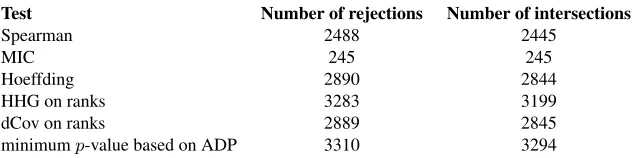
We compared these tests to seven tests of independence suggested in the literature. We compared
to Spearman’sρ, since it is perhaps the most widely used test to detect monotone associations. We
1. Normal vs. Normal with delta f1=N(0,1) f2= 0.8N(0,1)+0.2N(0.4,0.001)
2. Mix. vs. Mix., 3 vs. 4 Components f1= four Normal components at mu=−2,−0.2,0.2,2, sd=0.133 f2= 0.25(N(−1.93,0.198^2)+N(−1.93,0.039))+0.5N(0,0.039)
3. Normal vs. Normal with many deltas f1=N(0,1)
f2=0.8N(0,1) + 0.2 sampled from (−2,−1.5,−1,...,2)
4. Normal vs. Mixture 2 Components f1=N(0,1) f2=0.5(N(−0.866,0.25)+N(0.866,0.25))
5. Normal vs. Mixture 3 Components f1=N(0,1)
f2=1/3*(N(−1.122,0.16)+N(0,0.16)+N(1.122,0.16))
6. Normal vs. Mixture 5 Components f1=N(0,1)
f2=5 Normal Components,mu= (−1.369, −0.684, 0, 0.684, 1.369),sd=0.25
7. Cauchy, Shift f1=cauchy(0.17) f2=cauchy(−0.17)
8. Symmetric Gaussian mixture f1=N(0,2.967) f2=0.5(N(−0.85,1)+N(0.85,1))
9. Asymmetric Gaussian mixture f1=N(0.88, 2.061) f2=0.1*N(−1.1,1)+0.9*N(1.1,1)
10. Asymmetric Mixture vs. Mixture f1=0.5(N(−1, 0.1806)+N(1,0.36)) f2=0.5(N(−1.1,0.36)+N(1.1,0.180))
11. Mix. vs. Mix., 2 vs. 3 Components f1=1/2(N(−1,0.0174)+N(1,0.1089)) f2=1/3(N(−1.12,0.004356)+N(−0.88,0.004356)+N(0.9,0.1317))
12. Mix. vs. Mix., 2 vs. 4 Components, Symmetric f1=two Normal Components, mu=−1,1, sd=0.165 f2=four Normal components mu=−1.15,−0.85,0.85,1.15, sd=0.099
13. Mix. vs. Mix., 3 vs. 3 Components, Asymmetric f1=1/2N(−1, 0.039)+1/4(N(0.88,0.0068)+N(1.12,0.0068)) f2=1/4(N(−1.12,0.0068)+N(−0.88,0.0068))+1/2(N(1,0.039)
Figure 2: The two-sample problem in 13 different setups considered forN = 500, which differ in
Figure 3: Estimated power withN = 500sample points for theMm(black) andSm (grey)
statis-tics for m ∈ {2, . . . ,149} for the setups of Figure 2. The score per partition was the
likelihood ratio test statistic. The power of the minimump-value is the horizontal dashed
black line when it combines thep-values based onMm, and the horizontal dotted grey
line when it combines thep-values based onSm. The vertical lines show the optimalm
Min.p-value aggregation
Setup by Max by Sum Wilcox KS CVM AD HHG DS
1 Normal vs. Normal with delta 0.825 0.491 0.072 0.149 0.108 0.099 0.175 0.849 2 Mix. Vs. Mix., 3 Vs. 4 Components 0.799 0.873 0.000 0.020 0.001 0.021 0.344 0.560 3 Normal vs. Normal with many deltas 0.785 0.733 0.051 0.078 0.073 0.099 0.142 0.245 4 Normal vs. Mixture 2 Components 0.827 0.937 0.053 0.531 0.458 0.495 0.855 0.796 5 Normal vs. Mixture 5 Components 0.592 0.686 0.048 0.238 0.179 0.246 0.484 0.556 6 Normal vs. Mixture 10 Components 0.818 0.820 0.048 0.240 0.211 0.310 0.561 0.789 7 Cauchy, Shift 0.339 0.492 0.542 0.620 0.627 0.577 0.641 0.436 8 Symmetric Gaussian mixture 0.752 0.775 0.033 0.194 0.242 0.617 0.749 0.835 9 Asymmetric Gaussian mixture 0.512 0.613 0.050 0.253 0.277 0.469 0.678 0.599 10 Asymmetric Mixture vs. Mixture 0.711 0.806 0.000 0.159 0.119 0.395 0.690 0.747 11 Mix. Vs. Mix., 2 Vs. 3 Components 0.540 0.686 0.004 0.093 0.057 0.116 0.302 0.440 12 Mix. Vs. Mix., 2 Vs. 4 Comp., Sym. 0.390 0.577 0.000 0.005 0.000 0.005 0.079 0.270 13 Mix. Vs. Mix., 3 Vs. 3 Comp., Asym. 0.844 0.764 0.000 0.001 0.000 0.013 0.042 0.780
14 Null 0.051 0.051 0.050 0.043 0.050 0.050 0.050 0.050
Table 1: Power of competitors (columns 4-9), along with the minimump-value statistic using the
Mm p-values (column 2) and theSm p-values (column 3), forN = 500. The score per
partition was the likelihood ratio test statistic. The standard error was at most 0.0035.
The advantage of the test based on the minimum p-value is large when the number of
intersections of the two densities is at least four (setups 2,3,4,5,6,10,11,12, and 13). The
best competitors are HHG and DS, but HHG is essentially anm≤3test, and DS penalizes
largems severely, therefore in setups wherem ≥4partitions are better they can perform
poorly. Among the two variants in columns 2 and 3, the better choice clearly depends on the range of support in which the differences in distributions occur: aggregation by maximum has better power when the difference between the distributions is very local (setups 1, 3, and 13), and aggregation by summation has better power otherwise. The highest power per row is underlined.
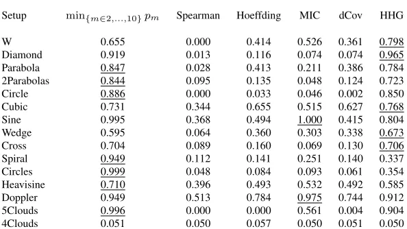
referred to as MIC, which is not consistent due to the computational shortcuts they have to use. We note that the power of the original dCov and HHG was fairly similar to the power of their distribution-free variants, see Appendix I.
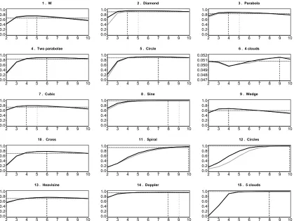
We examine complex bivariate relationships depicted in Figure 4. Most of these scenarios were collected from the literature illustrating the performance of other methods. Specifically, the first two rows were examined in Newton (2009), the next two rows are similar to the relationships ex-amined in Reshef et al. (2011), and the Heavisine and Doppler examples in the last row were used extensively in the literature on denoising, see e.g., Donoho and Johnstone (1995). In all but the 4 Independent Clouds setup, there is dependence. The 4 Independent Clouds setup allows us to
verify that the tests maintain the nominal level. We used 2000 simulated data sets forN = 100and
N = 300, in each of the configurations of Figure 4. Monotone setups are presented in Appendix H in Figure 12. Monotone setups are less interesting in the context of this work, because if there
is reason to believe that the dependence is monotone, specialized tests such as Spearman’s ρ or
Kendall’sτ will be preferable, but it is important to know that the suggested tests have reasonable
power, as demonstrated in the results in Appendix H, Figure 13 and Table 10.
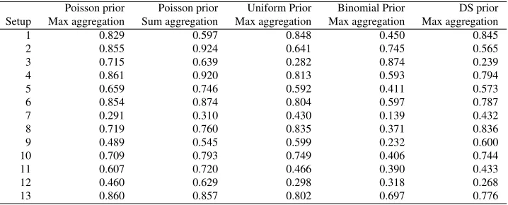
Tables 2 and 3, and Figure 5 show the power for the settings depicted in Figure 4. We only