Proto-value Functions: A Laplacian Framework for Learning Representation and Control in Markov Decision Processes

Proto-value Functions: A Laplacian Framework for Learning

Representation and Control in Markov Decision Processes

Sridhar Mahadevan [email protected]

Department of Computer Science University of Massachusetts Amherst, MA 01003, USA

Mauro Maggioni [email protected]

Department of Mathematics and Computer Science Duke University

Durham, NC 27708

Editor: Carlos Guestrin

Abstract

This paper introduces a novel spectral framework for solving Markov decision processes (MDPs) by jointly learning representations and optimal policies. The major components of the framework described in this paper include: (i) A general scheme for constructing representations or basis func-tions by diagonalizing symmetric diffusion operators (ii) A specific instantiation of this approach where global basis functions called proto-value functions (PVFs) are formed using the eigenvectors of the graph Laplacian on an undirected graph formed from state transitions induced by the MDP (iii) A three-phased procedure called representation policy iteration comprising of a sample collec-tion phase, a representacollec-tion learning phase that constructs basis funccollec-tions from samples, and a final parameter estimation phase that determines an (approximately) optimal policy within the (linear) subspace spanned by the (current) basis functions. (iv) A specific instantiation of the RPI frame-work using least-squares policy iteration (LSPI) as the parameter estimation method (v) Several strategies for scaling the proposed approach to large discrete and continuous state spaces, including the Nystr¨om extension for out-of-sample interpolation of eigenfunctions, and the use of Kronecker sum factorization to construct compact eigenfunctions in product spaces such as factored MDPs (vi) Finally, a series of illustrative discrete and continuous control tasks, which both illustrate the concepts and provide a benchmark for evaluating the proposed approach. Many challenges remain to be addressed in scaling the proposed framework to large MDPs, and several elaboration of the proposed framework are briefly summarized at the end.

Keywords: Markov decision processes, reinforcement learning, value function approximation, manifold learning, spectral graph theory

1. Introduction

This paper introduces a novel spectral framework for solving Markov decision processes (MDPs) (Puterman, 1994) where both the underlying representation or basis functions and (approximate) optimal policies within the (linear) span of these basis functions are simultaneously learned. This framework addresses a major open problem not addressed by much previous work in the field of

(Sutton and Barto, 1998), where the set of “features” or basis functions mapping a state s to a

k-dimensional real vectorφ(s)_∈Rkis usually hand-engineered.

The overall framework can be summarized briefly as follows. The underlying task environment is modeled as an MDP, where the system dynamics and reward function are typically assumed to be unknown. An agent explores the underlying state space by carrying out actions using some policy, say a random walk. Central to the proposed framework is the notion of a diffusion model (Coifman et al., 2005a; Kondor and Lafferty, 2002): the agent constructs a (directed or undirected) graph connecting states that are “nearby”. In the simplest setting, the diffusion model is defined by

the combinatorial graph Laplacian matrix L=D₋W , where W is a symmetrized weight matrix,

and D is a diagonal matrix whose entries are the row sums of W .1 Basis functions are derived

by diagonalizing the Laplacian matrix L, specifically by finding its “smoothest” eigenvectors that correspond to the smallest eigenvalues. Eigenvectors capture large-scale temporal properties of a transition process. In this sense, they are similar to value functions, which reflect the accumulation of rewards over the long run. The similarity between value functions and the eigenvectors of the graph Laplacian sometimes can be remarkable, leading to a highly compact encoding (measured in terms of the number of basis functions needed to encode a value function). Laplacian basis functions can be used in conjunction with a standard “black box” parameter estimation method, such as Q-learning (Watkins, 1989) or least-squares policy iteration (LSPI) (Lagoudakis and Parr, 2003) to find the best policy representable within the space of the chosen basis functions.

While the overall goal of learning representations is not new within the context of MDPs— it has been addressed by Dayan (1993) and Drummond (2002) among others—our approach is substantially different from previous work. The fundamental idea is to construct basis functions for solving MDPs by diagonalizing symmetric diffusion operators on an empirically learned graph representing the underlying state space. A diffusion model is intended to capture information flow

on a graph or a manifold.2 A simple diffusion model is a random walk on an undirected graph, where

the probability of transitioning from a vertex (state) to its neighbor is proportional to its degree, that

is Pr=D−1W (Chung, 1997). As we will see in Section 3, the combinatorial Laplacian operator L

defined in the previous paragraph is closely related spectrally to the random walk operator Pr. A key

advantage of diffusion models is their simplicity: it can be significantly easier to estimate a “weak”

diffusion model, such as the undirected random walk Pr or the combinatorial Laplacian L, than to

learn the true underlying transition matrix Pπof a policyπ.

The proposed framework can be viewed as automatically generating subspaces on which to project the value function using spectral analysis of operators on graphs. This differs fundamen-tally from many past attempts at basis function generation, for example tuning the parameters of pre-defined basis functions (Menache et al., 2005; Kveton and Hauskrecht, 2006), dynamically al-locating new parametric basis functions based on state space trajectories (Kretchmar and Anderson, 1999), or generating basis functions using the Bellman error in approximating a specific value func-tion (Keller et al., 2006; Petrik, 2007; Parr et al., 2007; Patrascu et al., 2002). The main contribufunc-tion

1. Section 9 describes how to generalize this simple diffusion model in several ways, including directed graphs where the symmetrization is based on the Perron vector or the leading eigenvector associated with the largest eigenvalue (Chung, 2005), state-action diffusion models where the vertices represent state-action pairs, and diffusion models for temporally extended actions.

of this paper is to show how to construct novel non-parametric basis functions whose shapes reflect the geometry of the environment.

In this paper, basis functions are constructed from spectral analysis of diffusion operators where the resulting representations are constructed without explicitly taking rewards into account. This approach can be contrasted with recent approaches that explicitly use reward information to generate basis functions (Keller et al., 2006; Petrik, 2007; Parr et al., 2007). There are clear advantages and disadvantages to these two approaches. In the non-reward based approach, basis functions can be more easily transferred across MDPs in situations where an agent is required to solve multiple tasks defined on a common state (action) space. Furthermore, basis functions constructed using spectral analysis reflect global geometric properties, such as bottlenecks and symmetries in state spaces, that are invariant across multiple MDPs on the same state (action) space. Finally, in the full control learning setting studied here, the agent does not initially know the true reward function or transition dynamics, and building representations based on estimating these quantities introduces another potential source of error. It is also nontrivial to learn accurate transition models, particularly in continuous MDPs. However, in other settings such as planning, where the agent can be assumed to have a completely accurate model, it is entirely natural and indeed beneficial to exploit reward or transition dynamics in constructing basis functions. In particular, it is possible to design algorithms for basis function generation with provable performance guarantees (Parr et al., 2007; Petrik, 2007), although these theoretical results are at present applicable only to the more limited case of evaluating a fixed policy. The proposed framework can in fact be easily extended to use reward information by building reward-based diffusion models, as will be discussed in more detail in Section 9.

Since eigenvectors of the graph Laplacian form “global” basis functions whose support is the en-tire state space, each eigenvector induces a real-valued mapping over the state space. Consequently, we can view each eigenvector as a “proto-value” function (or PVF), and the set of PVFs form the “building blocks” of all value functions on a state space (Mahadevan, 2005a). Of course, it is easy to construct a complete orthonormal set of basis functions spanning all value functions on a graph: the unit vectors themselves form such a basis, and indeed, any collection of_|S_|random vectors can (with high probability) be orthonormalized so that they are of unit length and “perpendicular” to each other. The challenge is to construct a compact basis set that is efficient at representing value functions with as few basis functions as possible. Proto-value functions differ from these obvious choices, or indeed other more common parametric choices such as radial basis functions (RBFs), polynomial bases, or CMAC, in that they are associated with the spectrum of the Laplacian which has an intimate relationship to the large-scale geometry of a state space. The eigenvectors of the Laplacian also provide a systematic organization of the space of functions on a graph, with the “smoothest” eigenvectors corresponding to the smallest eigenvalues (beginning with the constant function associated with the zero eigenvalue). By projecting a given value function on the space spanned by the eigenvectors of the graph Laplacian, the “spatial” content of a value function is mapped into a “frequency” basis, a hallmark of classical “Fourier” analysis (Mallat, 1989).

It has long been recognized that traditional parametric function approximators may have diffi-culty accurately modeling value functions due to nonlinearities in an MDP’s state space (Dayan,

1993). Figure 1 illustrates the problem with a simple example.3 In particular, as Dayan (1993) and

Drummond (2002) among others have noted, states close in Euclidean distance may have values that are very far apart (e.g., two states on opposite sides of a wall in a spatial navigation task). While

there have been several attempts to fix the shortcomings of traditional function approximators to address the inherent nonlinear nature of value functions, these approaches have lacked a sufficiently comprehensive and broad theoretical framework (related work is discussed in more detail in Sec-tion 8). We show that by rigorously formulating the problem of value funcSec-tion approximaSec-tion as

approximating real-valued functions on a graph or manifold using a diffusion model, a more

gen-eral solution emerges that not only has broader applicability than these previous methods, but also enables a novel framework called Representation Policy Iteration (RPI) (Mahadevan, 2005b) where representation learning is interleaved with policy learning. The RPI framework consists of an outer loop that learns basis functions from sample trajectories, and an inner loop that consists of a control learner that finds improved policies.

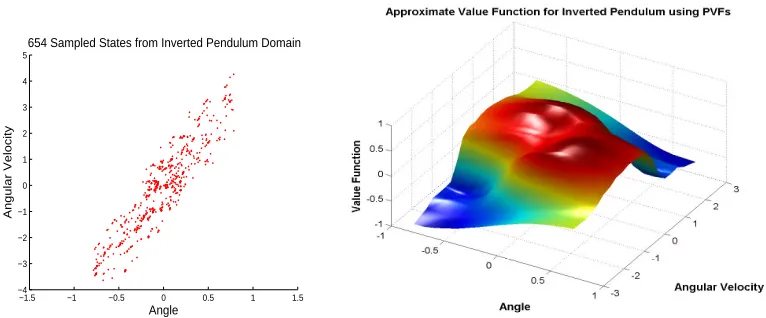
Figure 2 shows a set of samples produced by doing a random walk in the inverted pendulum task. In many continuous control tasks, there are often physical constraints that limit the “degrees of freedom” to a lower-dimensional manifold, resulting in motion along highly constrained regions of the state space. Instead of placing basis functions uniformly in all regions of the state space, the proposed framework recovers the underlying manifold by building a graph based on the samples collected over a period of exploratory activity. The basis functions are then computed by diagonal-izing a diffusion operator (the Laplacian) on the space of functions on the graph, and are thereby customized to the manifold represented by the state (action) space of a particular control task. In discrete MDPs, such as Figure 1, the problem is one of compressing the space of (value) functions

R|S|(orR|S|×|A|for action-value functions). In continuous MDPs, such as Figure 2, the correspond-ing problem is compresscorrespond-ing the space of square-integrable functions onR2, denoted asL2(R2). In short, the problem is one of dimensionality reduction not in the data space, but on the space of functions on the data.4

Both the discrete MDP shown in Figure 1 and the continuous MDP shown in Figure 2 have “in-accessible” regions of the state space, which can be exploited in focusing the function approximator to accessible regions. Parametric approximators, as typically constructed, do not distinguish be-tween accessible and inaccessible regions. Our approach goes beyond modeling just the reachable state space, in that it also models the local non-uniformity of a given region. This non-uniform mod-eling of the state space is facilitated by constructing a graph operator which models the local density across regions. By constructing basis functions adapted to the non-uniform density and geometry of the state space, our approach extracts significant topological information from trajectories. These ideas are formalized in Section 3.

The additional power obtained from knowledge of the underlying state space graph or mani-fold comes at a potentially significant cost: the manimani-fold representation needs to be learned, and furthermore, basis functions need to be computed from it. Although our paper demonstrates that eigenvector-type basis functions resulting from a diffusion analysis of graph-based manifolds can solve standard benchmark discrete and continuous MDPs, the problem of efficiently learning mani-fold representations of arbitrary MDPs is beyond the scope of this introductory paper. We discuss a number of outstanding research questions in Section 9 that need to be addressed in order to develop a more complete solution.

One hallmark of Fourier analysis is that the basis functions are localized in frequency, but not in time (or space). Hence, the eigenfunctions of the graph Laplacian are localized in frequency by being associated with a specific eigenvalueλ, but their support is in general the whole graph. This

0 2 4 6 8 10 0 1 2 3 4 5 6 7 8 9 10 11

Total states = 100,"Wall" States = 47 G

Two−Room MDP using Unit Vector Bases

1 2 3 4 5 6 7 8 9 10 1 2 3 4 5 6 7 8 9 10 10 20 30 40 50 60 70 80 90 G 0 2 4 6 8 10 0 2 4 6 8 10 0 20 40 60 80 100

Optimal Value Function for Two−Room MDP

Figure 1: It is difficult to approximate nonlinear value functions using traditional parametric func-tion approximators. Left: a “two-room” environment with 100 total states, divided into 57 accessible states (including one doorway state), and 43 inaccessible states represent-ing exterior and interior walls (which are “one state” thick). Middle: a 2D view of the optimal value function for the two-room grid MDP, where the agent is (only) rewarded

for reaching the state marked G by+100. Access to each room from the other is only

available through a central door, and this “bottleneck” results in a strongly nonlinear op-timal value function. Right: a 3D plot of the opop-timal value function, where the axes are reversed for clarity.

−1.5 −1 −0.5 0 0.5 1 1.5 −4 −3 −2 −1 0 1 2 3 4 5

654 Sampled States from Inverted Pendulum Domain

Angle

Angular Velocity

Figure 2: Left: Samples from a series of random walks in an inverted pendulum task. Due to physical constraints, the samples are largely confined to a narrow region. The proto-value function framework presented in this paper empirically models the underlying manifold in such continuous control tasks, and derives customized basis functions that exploit the unique structure of such point-sets inRn_{. Right: An approximation of the value function}

global characteristic raises a natural computational concern: can Laplacian bases be computed and

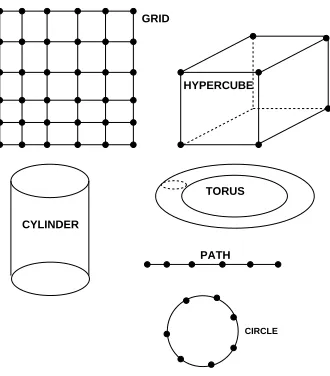
represented compactly in large discrete and continuous spaces?5 We will address this problem in

particular cases of interest: large factored spaces, such as grids, hypercubes, and tori, lead natu-rally to product spaces for which the Laplacian bases can be constructed efficiently using tensor

products. For continuous domains, by combining low-rank approximations and the Nystr ¨om

inter-polation method, Laplacian bases can be constructed quite efficiently (Drineas and Mahoney, 2005). Finally, a variety of other techniques can be used to sparsify Laplacian bases, including graph par-titioning (Karypis and Kumar, 1999), matrix sparsification (Achlioptas et al., 2002), and automatic Kronecker matrix factorization (Van Loan and Pitsianis, 1993). Other sources of information can be additionally exploited to facilitate sparse basis construction. For example, work on hierarchical reinforcement learning surveyed in Barto and Mahadevan (2003) studies special types of MDPs called semi-Markov decision processes, where actions are temporally extended, and value functions are decomposed using the hierarchical structure of a task. In Section 9, we discuss how to exploit such additional knowledge in the construction of basis functions.

This research is related to recent work on manifold and spectral learning (Belkin and Niyogi, 2004; Coifman and Maggioni, 2006; Roweis and Saul, 2000; Tenenbaum et al., 2000). A major difference is that our focus is on solving Markov decision processes. Value function approximation in MDPs is related to regression on graphs (Niyogi et al., 2003) in that both concern approximation of real-valued functions on the vertices of a graph. However, value function approximation is fun-damentally different since target values are initially unknown and must be determined by solving the Bellman equation, for example by iteratively finding a fixed point of the Bellman backup opera-tor. Furthermore, the set of samples of the manifold is not given a priori, but is determined through active exploration by the agent. Finally, in our work, basis functions can be constructed multiple times by interleaving policy improvement and representation learning. This is in spirit similar to the design of kernels adapted to regression or classification tasks (Szlam et al., 2006).

The rest of the paper is organized as follows. Section 2 gives a quick summary of the main framework called Representation Policy Iteration (RPI) for jointly learning representations and policies, and illustrates a simplified version of the overall algorithm on the small two-room dis-crete MDP shown earlier in Figure 1. Section 3 motivates the use of the graph Laplacian from several different points of view, including as a spectral approximation of transition matrices, as well as inducing a smoothness regularization prior that respects the topology of the state space through a data-dependent kernel. Section 4 describes a concrete instance of the RPI framework using least-squares policy iteration (LSPI) (Lagoudakis and Parr, 2003) as the underlying control learning method, and compares PVFs with two parametric bases—radial basis functions (RBFs) and polynomials—on small discrete MDPs. Section 5 describes one approach to scaling proto-value functions to large discrete product space MDPs, using the Kronecker sum matrix factorization method to decompose the eigenspace of the combinatorial Laplacian. This section also compares PVFs against RBFs on the Blockers task (Sallans and Hinton, 2004). Section 6 extends PVFs to con-tinuous MDPs using the Nystr ¨om extension for interpolating eigenfunctions from sampled states to novel states. A detailed evaluation of PVFs in continuous MDPs is given in Section 7, including

EXIT SAMPLE

COLLECTION

POLICY

LEARNING

CONSTRUCTION BASIS

Error tolerance

function Similarity Initial task specification

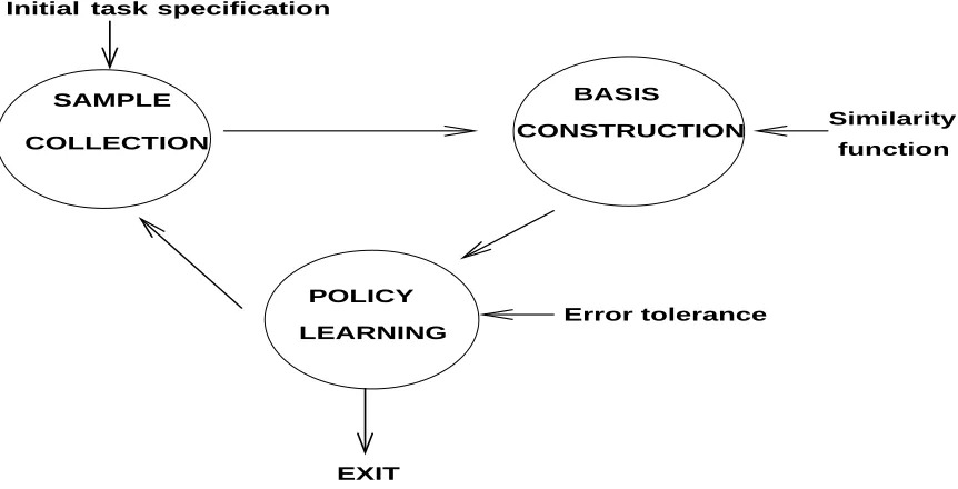
Figure 3: Flowchart of the unified approach to learning representation and behavior.

the inverted pendulum, the mountain car, and the Acrobot tasks (Sutton and Barto, 1998). Sec-tion 8 contains a brief descripSec-tion of previous work. SecSec-tion 9 discusses several ongoing extensions of the proposed framework, including Kronecker product matrix factorization (Johns et al., 2007), multiscale diffusion wavelet bases (Mahadevan and Maggioni, 2006), and more elaborate diffusion models using directed graphs where actions are part of the representation (Johns and Mahadevan, 2007; Osentoski and Mahadevan, 2007).

2. Overview of The Framework

This section contains a brief summary of the overall framework, which we call Representation

Policy Iteration (RPI) (Mahadevan, 2005b).6 Figure 3 illustrates the overall framework. There

are three main components: sample collection, basis construction, and policy learning. Sample collection requires a task specification, which comprises of a domain simulator (or alternatively a physically embodied agent like a robot), and an initial policy. In the simplest case, the initial policy can be a random walk, although it can also reflect a more informative hand-coded policy. The second phase involves constructing the bases from the collected samples using a diffusion model, such as an undirected (or directed) graph. This process involves finding the eigenvectors of a symmetrized graph operator such as the graph Laplacian. The final phase involves estimating the “best” policy representable in the span of the basis functions constructed (we are primarily restricting our attention to linear architectures, where the value function is a weighted linear combination of the bases). The entire process can then be iterated.

Figure 4 specifies a more detailed algorithmic view of the overall framework. In the sample collection phase, an initial random walk (perhaps guided by an informed policy) is carried out to

obtain samples of the underlying manifold on the state space. The number of samples needed is an empirical question which will be investigated in further detail in Section 5 and Section 6. Given this set of samples, in the representation learning phase, an undirected (or directed) graph is constructed in one of several ways: two states can be connected by a unit cost edge if they represent temporally successive states; alternatively, a local distance measure such as k-nearest neighbor can be used to connect states, which is particularly useful in the experiments on continuous domains reported in Section 7. From the graph, proto-value functions are computed using one of the graph operators discussed below, for example the combinatorial or normalized Laplacian. The smoothest eigenvectors of the graph Laplacian (that is, associated with the smallest eigenvalues) are used to form the suite of proto-value functions. The number of proto-value functions needed is a model selection question, which will be empirically investigated in the experiments described later. The encodingφ(s): S_→Rk of a state is computed as the value of the k proto-value functions on that state. To compute a state action encoding, a number of alternative strategies can be followed: the figure shows the most straightforward method of simply replicating the length of the state encoding by the number of actions and setting all the vector components to 0 except those associated with the current action. More sophisticated schemes are possible (and necessary for continuous actions), and will be discussed in Section 9.

At the outset, it is important to point out that the algorithm described in Figure 4 is one of many possible designs that combine the learning of basis functions and policies. In particular, the RPI framework is an iterative approach, which interleaves the two phases of generating basis functions by sampling trajectories from policies, and then subsequently finding improved policies from the augmented set of basis functions. It may be possible to design alternative frameworks where basis functions are learned jointly with learning policies, by attempting to optimize some cumulative measure of optimality. We discuss this issue in more depth in Section 9.

2.1 Sample Run of RPI on the Two-Room Environment

The result of running the algorithm is shown in Figure 5, which was obtained using the following specific parameter choices.

• The state space of the two room MDP is as shown in Figure 1. There are 100 states totally,

of which 43 states are inaccessible since they represent interior and exterior walls. The re-maining 57 states are divided into 1 doorway state and 56 interior room states. The agent

is rewarded by +100 for reaching state 89, which is the last accessible state in the bottom

right-hand corner of room 2. In the 3D value function plots shown in Figure 5, the axes are reversed to make it easier to visualize the value function plot, making state 89 appear in the top left (diagonally distant) corner.

• 3463 samples were collected using off-policy sampling from a random walk of 50 episodes,

each of length 100 (or terminating early when the goal state was reached).7 Four actions

(compass direction movements) were possible from each state. Action were stochastic. If a

movement was possible, it succeeded with probability 0.9. Otherwise, the agent remained in

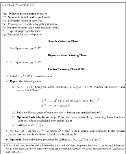
RPI(πm,T,N,ε,k,O,µ,D):

//πm: Policy at the beginning of trial m

// T : Number of initial random walk trials // N: Maximum length of each trial

//ε: Convergence condition for policy iteration // k: Number of proto-value basis functions to use //O: Type of graph operator used

// µ: Parameter for basis adaptation //D: Initial set of samples

Sample Collection Phase

1. Off-policy or on-policy sampling: Collect a data set of samplesDm={(si,ai,si+1,ri), . . .}by either

randomly choosing actions (off-policy) or using the supplied initial policy (on-policy) for a set of T trials, each of maximum N steps (terminating earlier if it results in an absorbing goal state), and add these transitions to the complete data setD.

2. (Optional) Subsampling step: Form a subset of samplesDs⊆D by some subsampling method

such as random subsampling or trajectory subsampling. For episodic tasks, optionally prune the trajectories stored inDsso that only those that reach the absorbing goal state are retained.

Representation Learning Phase

3. Build a diffusion model from the data in Ds. In the simplest case of discrete MDPs, construct an

undirected weighted graph G fromDby connecting state i to state j if the pair(i,j)form temporally successive states_∈S. Compute the operatorOon graph G, for example the normalized Laplacian

L=D−12(_D−_W)_D−12_.

4. Compute the k smoothest eigenvectors ofO on the graph G. Collect them as columns of the basis function matrixΦ, a_|S_{| ×}k matrix. The state action basesφ(s,a)can be generated from rows of this matrix by duplicating the state basesφ(s)|A_|times, and setting all the elements of this vector to 0 except for the ones corresponding to the chosen action.a

Control Learning Phase

5. Using a standard parameter estimation method (e.g., Q-learning or LSPI), find anε-optimal policyπ that maximizes the action value function Qπ=Φwπwithin the linear span of the basesΦusing the training data inD.

6. Optional: Set the initial policyπm+1toπand callRPI(πm+1,T,N,ε,k,O,µ,D).

a. In large continuous and discrete MDPs, the basis matrixΦneed not be explicitly formed and the featuresφ(s,a)

can be computed “on demand” as will be explained later.

the same state. When the agent reaches state 89, it receives a reward of 100, and is randomly reset to an accessible interior state.

• An undirected graph was constructed from the sample transitions, where the weight matrix W

is simply the adjacency (0,1) matrix. The graph operator used was the normalized Laplacian

L

2, where L=D−W is referred to as the combinatorial Laplacian (these graph

operators are described in more detail in Section 3).

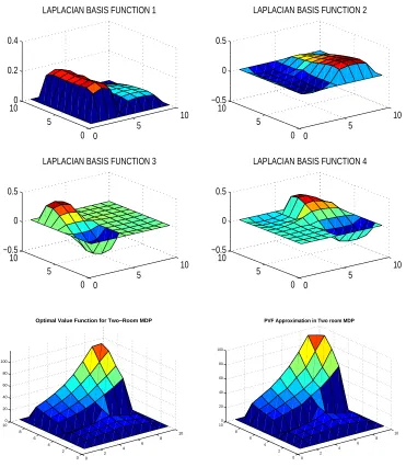
• 20 eigenvectors corresponding to the smallest eigenvalues of

L

for each action) are chosen as the columns of the state action basis matrixΦ. For example,

the first four eigenvectors are shown in Figure 5. These eigenvectors are orthonormal: they are normalized to be of length 1 and are mutually perpendicular. Note how the eigenvectors are sensitive to the geometric structure of the overall environment. For example, the second eigenvector allows partitioning the two rooms since it is negative for all states in the first room, and positive for states in the second room. The third eigenvector is non-constant over only one of the rooms. The connection between the Laplacian and regularities such as symmetries and bottlenecks is discussed in more detail in Section 3.6.

• The parameter estimation method used was least-squares policy iteration (LSPI), withγ=0.8. LSPI is described in more detail in Section 4.1.

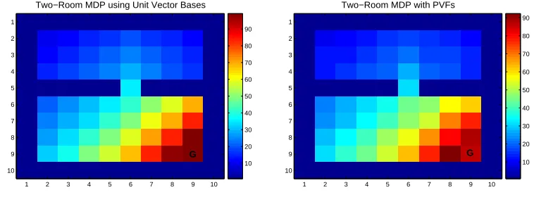
• The optimal value function using unit vector bases and the approximation produced by 20

PVFs are compared using the 2D array format in Figure 6.

In the remainder of this paper, we will evaluate this framework in detail, providing some ra-tionale for why the Laplacian bases are adept at approximating value functions, and demonstrating how to scale the approach to large discrete MDPs as well as continuous MDPs.

3. Representation Learning by Diffusion Analysis

In this section, we discuss the graph Laplacian, specifically motivating its use as a way to construct basis functions for MDPs. We begin with a brief introduction to MDPs, and then describe the spec-tral analysis of a restricted class of MDPs where the transition matrix is diagonalizable. Although this approach is difficult to implement for general MDPs, it provides some intuition into why eigen-vectors are a useful way to approximate value functions. We then introduce the graph Laplacian as a symmetric matrix, which acts as a surrogate for the true transition matrix, but which is easily diagonalizable. It is possible to model non-symmetric actions and policies using more sophisticated symmetrization procedures (Chung, 2005), and we postpone discussion of this extension to Sec-tion 9. There are a number of other perspectives to view the graph Laplacian, namely as generating a data-dependent reproducing kernel Hilbert space (RKHS) (Scholkopf and Smola, 2001), as well as a way to generate nonlinear embeddings of graphs. Although a full discussion of these perspectives is beyond this paper, they are worth noting in order to gain deeper insight into the many remarkable properties of the Laplacian.

3.1 Brief Overview of MDPs

0 5 10 0 5 100 0.2 0.4

LAPLACIAN BASIS FUNCTION 1

0 5 10 0 5 10 −0.5 0 0.5

LAPLACIAN BASIS FUNCTION 2

0 5 10 0 5 10 −0.5 0 0.5

LAPLACIAN BASIS FUNCTION 3

0 5 10 0 5 10 −0.5 0 0.5

LAPLACIAN BASIS FUNCTION 4

0 2 4 6 8 10 0 2 4 6 8 10 0 20 40 60 80 100

Optimal Value Function for Two−Room MDP

0 2 4 6 8 10 0 2 4 6 8 10 0 20 40 60 80 100

PVF Approximation in Two room MDP

Two−Room MDP using Unit Vector Bases

1 2 3 4 5 6 7 8 9 10 1 2 3 4 5 6 7 8 9 10 10 20 30 40 50 60 70 80 90 G

Two−Room MDP with PVFs

1 2 3 4 5 6 7 8 9 10 1 2 3 4 5 6 7 8 9 10 10 20 30 40 50 60 70 80 90 G

Figure 6: Left: the optimal value function for the two-room MDP using unit vector bases. Right: approximation with 20 PVFs using the RPI algorithm.

s0 when an action a is performed in state s, and a corresponding reward model Ra_ss0 specifying a scalar cost or reward (Puterman, 1994). In continuous Markov decision processes, the set of states

⊆Rd. Abstractly, a value function is a mapping S_→Ror equivalently (in discrete MDPs) a vector

∈R|S|. Given a policyπ: S_→A mapping states to actions, its corresponding value function Vπ

specifies the expected long-term discounted sum of rewards received by the agent in any given state

s when actions are chosen using the policy. Any optimal policyπ∗defines the same unique optimal

value function V∗which satisfies the nonlinear constraints

V∗(s) =T∗(V∗(s)) =max

a Rsa+γ

∑

s0_∈S

P_ssa0V∗(s0)

!

,

where Rsa=∑s0_∈sP_ssa0Ra_ss0 is the expected immediate reward. Value functions are mappings from the state space to the expected long-term discounted sum of rewards received by following a fixed (deterministic or stochastic) policyπ. Here, T∗can be viewed as an operator on value functions, and

V∗represents the fixed point of the operator T∗. The value function Vπassociated with following a (deterministic) policyπcan be defined as

Vπ(s) =T(Vπ(s)) =R_sπ(s)+γ

∑

s0_∈S

P_ssπ(0s)Vπ(s0).

Once again, T is an operator on value functions, whose fixed point is given by Vπ. Value

functions in an MDP can be viewed as the result of rewards “ diffusing” through the state space, governed by the underlying system dynamics. Let Pπrepresent an _|S_{| × |}S_|transition matrix of a (deterministic) policyπ: S_→A mapping each state s_∈S to a desired action a=π(s). Let Rπbe a (column) vector of size_|S_|of rewards. The value function associated with policyπcan be defined using the Neumann series:

Vπ= (I₋γPπ)−1_Rπ_{= I+γP}π_+γ2_(Pπ₎2_{+. . .}

3.2 Approximation of Value Functions

It is obviously difficult to represent value functions exactly on large discrete state spaces, or in continuous spaces. Consequently, there has been much study of approximation architectures for representing value functions (Bertsekas and Tsitsiklis, 1996). Value functions generally exhibit two key properties: they are typically smooth, and they reflect the underlying state space geometry. A fundamental contribution of this paper is the use of an approximation architecture that exploits a new notion of smoothness, not in the traditional sense of Euclidean space, but smoothness on the state space graph. The notion of smooth functions on graphs can be formalized using the Sobolev norm (Mahadevan and Maggioni, 2006). In addition, value functions usually reflect the geometry of the environment (as illustrated in Figure 5). Smoothness derives from the fact that the value at a given state Vπ(s)is always a function of values at “neighboring” states. Consequently, it is natural to construct basis functions for approximating value functions that share these two properties.8

Let us define a set of basis functions F_Φ=_{φ1, . . . ,φk}, where each basis function represents

a “feature”φi: S→R. The basis function matrixΦis an |S| ×k matrix, where each column is a

particular basis function evaluated over the state space, and each row is the set of all possible basis

functions evaluated on a particular state. Approximating a value function using the matrixΦcan be

viewed as projecting the value function onto the column space spanned by the basis functionsφi,

Vπ_≈Vˆπ=Φwπ=

∑

i

wπ_iφi.

Mathematically speaking, this problem can be rigorously formulated using the framework of best approximation in inner product spaces (Deutsch, 2001). In fact, it is easy to show that the space of value functions represents a Hilbert space, or a complete inner product space (Van Roy, 1998).

For simplicity, we focus on the simpler problem of approximating a fixed policyπ, which defines a

Markov chain whereρπrepresents its invariant (long-term) distribution. This distribution defines a Hilbert space, where the inner product is given by

hV1,V2iπ=

∑

V₁π(s)V₂π(s)ρπ(s).

The “length” or norm in this inner product space is defined as_kV_kπ=p

hV,V_iπ. Value function ap-proximation can thus be formalized as a problem of best apap-proximation in a Hilbert space (Deutsch,

2001). It is well known that if the basis functions φi are orthonormal (unit-length and mutually

perpendicular), the best approximation of the value function Vπcan be expressed by its projection

onto the space spanned by the basis functions, or more formally

Vπ_≈

∑

i∈I

hVπ,φiiπφi,

where I is the set of indices that define the basis set. In finite MDPs, the best approximation can be characterized using the weighted least-squares projection matrix

Mπ_Φ=Φ(ΦTDρπΦ)−1ΦTDρπ,

where Dρπ is a diagonal matrix whose entries represent the distributionρπ. We know the Bellman “backup” operator T defined above has a fixed point Vπ=T(Vπ). Many standard parameter estima-tion methods, including LSPI (Lagoudakis and Parr, 2003) and LSTD (Bradtke and Barto, 1996), can be viewed as finding an approximate fixed point of the operator T

ˆ

Vπ=Φwπ=M_φπ(T(Φwπ)).

It can be shown that the operator T is a contraction mapping, where

kTV1−TV2kπ≤γkV1−V2kπ.

A natural question that arises is whether we can quantify the error in value function approximation under a set of basis functions F_φ. Exploiting the contraction property of the operator T under the norm defined by the weighted inner product, it can be shown that the “distance” between the true value function Vπand the fixed point ˆVπcan be bounded in terms of the distance between Vπand its projection onto the space spanned by the basis functions (Van Roy, 1998):

kVπ₋Vˆπ_kπ≤₁ 1 −κ2kV

π_−Mπ φVπkπ,

where κis the contraction rate defined by Bellman operator T in conjunction with the weighted

least-squares projection.

The problem of value function approximation in control learning is significantly more difficult, in that it involves finding an approximate fixed point of the initially unknown operator T∗. One stan-dard algorithm for control learning is approximate policy iteration (Bertsekas and Tsitsiklis, 1996), which interleaves an approximate policy evaluation step of finding an approximation of the value function ˆVπk_{associated with a given policy}π

kat stage k, with a policy improvement step of finding

the greedy policy associated with ˆVπk_{. Here, there are two sources of error introduced by} approx-imating the exact value function, and approxapprox-imating the policy. We will describe a specific type of approximate policy iteration method—the LSPI algorithm (Lagoudakis and Parr, 2003)—in Sec-tion 4, which uses a least-squares approach to approximate the acSec-tion-value funcSec-tion. An addiSec-tional problem in control learning is that the standard theoretical results for approximate policy iteration are often expressed in terms of the maximum (normed) error, whereas approximation methods are most naturally formulated as projections in a least-squared normed space. There continues to be work on developing more useful weighted least-square bounds, although these currently assume the policy is exactly representable (Munos, 2003, 2005). Also, it is possible to design approximation methods that directly carry out max-norm projections using linear programming, although this work usually assumes the transition dynamics is known (Guestrin et al., 2001),

3.3 Spectral Analysis of Transition Matrices

In this paper, the orthogonal basis functions are constructed in the Fourier tradition by diagonalizing an operator (or matrix) and finding its eigenvectors. We motivate this approach by first assuming that the eigenvectors are constructed directly from a (known) state transition matrix Pπand show that if

the reward function Rπis known, the eigenvectors can be selected nonlinearly based on expanding

the value function Vπ on the eigenvectors of the transition matrix. Petrik (2007) develops this

line of reasoning, assuming that Pπ and Rπ are both known, and that Pπ is diagonalizable. We

describe this perspective in more detail below as it provides a useful motivation for why we use diagonalizable diffusion matrices instead. One subclass of diagonalizable transition matrices are those corresponding to reversible Markov chains (which will turn out to be useful below). Although transition matrices for general MDPs are not reversible, and their spectral analysis is more delicate, it will still be a useful starting point to understand diffusion matrices such as the graph Laplacian.9 If the transition matrix Pπis diagonalizable, there is a complete set of eigenvectorsΦπ= (φπ₁, . . .φπ_n)

that provides a change of basis in which the transition matrix Pπ is representable as a diagonal

matrix. For the sub-class of diagonalizable transition matrices represented by reversible Markov chains, the transition matrix is not only diagonalizable, but there is also an orthonormal basis. In other words, using a standard result from linear algebra, we have

Pπ=ΦπΛπ(Φπ)T,

whereΛπis a diagonal matrix of eigenvalues. Another way to express the above property is to write the transition matrix as a sum of projection matrices associated with each eigenvalue:

Pπ=

n

∑

λπ

iφπi(φπi)T,

where the eigenvectorsφπ_i form a complete orthogonal basis (i.e.,_kφπ_{i k}2=1 andhφπi,φπji=0,i6=j).

It readily follows that powers of Pπhave the same eigenvectors, but the eigenvalues are raised to the corresponding power (i.e.,(Pπ)k_φπ

i = (λπi)kφπi). Since the basis matrixΦspans all vectors on the

state space S, we can express the reward vector Rπin terms of this basis as

Rπ=Φπαπ, (2)

whereαπis a vector of scalar weights. For high powers of the transition matrix, the projection ma-trices corresponding to the largest eigenvalues will dominate the expansion. Combining Equation 2

with the Neumann expansion in Equation 1, we get

Vπ =

∞

∑

(γPπ)i_Φπ_απ

=

∞

∑

n

∑

γi_(Pπ₎i_φπ kαπk

=

n

∑

∞

∑

γi_(λπ k)

i_φπ kαπk

=

n

∑

1 1−γλπk

φπ kαπk

=

n

∑

βkφπk,

where we used the property that(Pπ)i_φπ

j= (λπj)iφπj. Essentially, the value function Vπis represented

as a linear combination of eigenvectors of the transition matrix. In order to provide the most

effi-cient approximation, we can truncate the summation by choosing some small number m<n of the

eigenvectors, preferably those for whom βk is large. Of course, since the reward function is not

known, it might be difficult to pick a priori those eigenvectors that result in the largest coefficients. A simpler strategy instead is to focus on those eigenvectors for whom the coefficients _1−γλ1 π

k are the largest. In other words, we should pick the eigenvectors corresponding to the largest eigenvalues of the transition matrix Pπ(since the spectral radius is 1, the eigenvalues closest to 1 will dominate the smaller ones):

Vπ_≈

m

∑

1 1₋γλπ_kφ

π

kαπk, (3)

where we assume the eigenvalues are ordered in non-increasing order, soλπ₁is the largest eigenvalue. If the transition matrix Pπand reward function Rπare both known, one can of course construct basis

functions by diagonalizing Pπand choosing eigenvectors “out-of-order” (that is, pick eigenvectors

with the largest βk coefficients above). Petrik (2007) shows a (somewhat pathological) example

where a linear spectral approach specified by Equation 3 does poorly when the reward vector is chosen such that it is orthogonal to the first k basis functions. It is an empirical question whether such pathological reward functions exhibit themselves in more natural situations. The repertoire of discrete and continuous MDPs we study seem highly amenable to the linear spectral decomposition approach. However, we discuss various approaches for augmenting PVFs with reward-sensitive bases in Section 9.

The spectral approach of diagonalizing the transition matrix is problematic for several reasons.

One, the transition matrix Pπcannot be assumed to be symmetric, in which case one has to deal

7

1

2

3

4

5

6

7

Goal

1

6

2

3

5

4

Pr=



  

0 0.5 0.5 0 0 0 0

0.5 0 0 0.5 0 0 0

0.33 0 0 0.33 0.33 0 0

. . .



  

Figure 7: Top: A simple diffusion model given by an undirected unweighted graph connecting each state to neighbors that are reachable using a single (reversible) action. Bottom: first three rows of the random walk matrix Pr=D−1W . Pr is not symmetric, but it has

real eigenvalues and eigenvectors since it is spectrally related to the normalized graph Laplacian.

3.4 From Transition Matrices to Diffusion Models

We now develop a line of analysis where a graph is induced from the state space of an MDP, by sampling from a policy such as a random walk. Let us define a weighted graph G= (V,E,W), where

V is a finite set of vertices, and W is a weighted adjacency matrix with W(i,j)>0 if(i,j)_∈E, that is

it is possible to reach state i from j (or vice-versa) in a single step. A simple example of a diffusion

model on G is the random walk matrix Pr=D−1W . Figure 7 illustrates a random walk diffusion

model. Note the random walk matrix Pr=D−1W is not symmetric. However, it can be easily shown

that Prdefines a reversible Markov chain, which induces a Hilbert space with respect to the inner

product defined by the invariant distributionρ:

hf,g_iρ=

∑

v∈V

f(i)g(i)ρ(i).

In addition, the matrix Pr can be shown to be self-adjoint (symmetric) with respect to the above

inner product, that is

hPrf,giρ=hf,Prgiρ.

Consequently, the matrix Prcan be shown to have real eigenvalues and orthonormal eigenvectors,

with respect to the above inner product.

The random walk matrix Pr=D−1W is called a diffusion model because given any function f on

the underlying graph G, the powers of P_rtf determine how quickly the random walk will “mix” and

of a random walk on an undirected graph is given byρ(v) = dv

vol(G), where dvis the degree of vertex

v and the “volume” vol(G) =∑_v∈Gdv. Even though the random walk matrix Prcan be diagonalized,

for computational reasons, it turns out to be highly beneficial to find a symmetric matrix with a closely related spectral structure. This is essentially the graph Laplacian matrix, which we now describe in more detail.

3.5 The Graph Laplacian

For simplicity, assume the underlying state space is represented as an undirected graph G= (V,E,W), where V is the set of vertices, E is the set of edges where(u,v)_∈E denotes an undirected edge from

vertex u to vertex v. The more general case of directed graphs is discussed in Section 9.3. The

com-binatorial Laplacian L is defined as the operator L=D₋W , where D is a diagonal matrix called

the valency matrix whose entries are row sums of the weight matrix W . The first three rows of the combinatorial Laplacian matrix for the grid world MDP in Figure 7 is illustrated below, where we assume a unit weight on each edge:

L=



  

2 ₋1 ₋1 0 0 0 0

−1 2 0 ₋1 0 0 0

−1 0 3 ₋1 ₋1 0 0

. . .



  

.

Comparing the above matrix with the random walk matrix in Figure 7, it may seem like the two matrices have little in common. Surprisingly, we will show that there is indeed an intimate connection between the random walk matrix and the Laplacian. The Laplacian has many attractive spectral properties. It is both symmetric as well as positive semi-definite, and hence its eigenvalues are not only all real, but also non-negative. It is useful to view the Laplacian as an operator on the space of functions

F

L f(i) =

∑

j∼i

(f(i)₋f(j)),

that is the Laplacian acts as a difference operator. On a two-dimensional grid, the Laplacian can be shown to essentially be a discretization of the continuous Laplace operator

∂2_f ∂x2+

∂2_f ∂y2,

where the partial derivatives are replaced by finite differences.

Another fundamental property of the graph Laplacian is that projections of functions on the eigenspace of the Laplacian produce the smoothest global approximation respecting the underlying graph topology. More precisely, let us define the inner product of two functions f and g on a graph as_hf,g_i=∑_uf(u)g(u).10 _{Then, it is easy to show that}

hf,L f_i=

∑

u∼v

wuv(f(u)−f(v))2,

where this so-called Dirichlet sum is over the (undirected) edges u∼v of the graph G, and wuv

denotes the weight on the edge. Note that each edge is counted only once in the sum. From the standpoint of regularization, this property is crucial since it implies that rather than smoothing using properties of the ambient Euclidean space, smoothing takes the underlying manifold (graph) into account.

To make the connection between the random walk operator Printroduced in the previous section,

and the Laplacian, we need to introduce the normalized Laplacian (Chung, 1997), which is defined as

L

To see the connection between the normalized Laplacian and the random walk matrix Pr=

D−1W , note the following identities:

L

2 =I−D− 1 2W D−

1 2,

I₋

L

1 2,

D−12(I−

L

2 = D−1W.

Hence, the random walk operator D−1W is similar to I₋

L

L

by D−21. We can now provide a rationale for choosing the eigenvectors of the Laplacian as basis

functions. In particular, ifλiis an eigenvalue of the random walk transition matrix Pr, then 1−λiis

the corresponding eigenvalue of

L

select the eigenvectors of the normalized graph Laplacian corresponding to the smallest eigenvalues.

The normalized Laplacian

L

is

L

duv

∑

f(u) √

du −

f(v) √

dv

wuv.

The difference between the combinatorial and normalized Laplacian is that the latter models the degree of a vertex as a local measure. In Section 7, we provide an experimental evaluation of the different graph operators for solving continuous MDPs.

Building on the Dirichlet sum above, a standard variational characterization of eigenvalues and eigenvectors views them as the solution to a sequence of minimization problems. In particular, the set of eigenvalues can be defined as the solution to a series of minimization problems using the Rayleigh quotient (Chung, 1997). This provides a variational characterization of eigenvalues

using projections of an arbitrary function g : V _→

R

L

eigenvalues and the functions satisfying orthonormality are the eigenfunctions:

hg,Lg_i

hg,g_i =

hg,D−12LD− 1 2gi

hg,g_i =

∑u∼v(f(u)−f(v))2wuv ∑uf2(u)du

,

where f_≡D−12g. The first eigenvalue isλ₀=0, and is associated with the constant function f(u) = 1, which means the first eigenfunction go(u) =

√

D 1 (for an example of this eigenfunction, see top

g : V →

R

eigenvalueλ1, namely

λ1= inf f_⊥√D1

∑u∼v(f(u)−f(v))2wuv ∑uf2(u)du

.

The Rayleigh quotient for higher-order basis functions is similar: each function is perpendicular to the subspace spanned by previous functions (see top four plots in Figure 5). In other words, the eigenvectors of the graph Laplacian provide a systematic organization of the space of functions on a graph that respects its topology.

3.6 Proto-Value Functions and Large-Scale Geometry

We now formalize the intuitive notion of why PVFs capture the large-scale geometry of a task environment, such as its symmetries and bottlenecks. A full discussion of this topic is beyond the scope of this paper, and we restrict our discussion here to one interesting property connected to

the automorphisms of a graph. Given a graph G= (V,E,W), an automorphismπof a graph is a

bijectionπ: V _→V that leaves the weight matrix invariant. In other words, w(u,v) =w(π(u),π(v)).

An automorphismπcan be also represented in matrix form by a permutation matrixΓthat commutes

with the weight matrix:

ΓW=WΓ.

An immediate consequence of this property is that automorphisms leave the valency, or degree of a vertex, invariant, and consequently, the Laplacian is invariant under an automorphism. The set of all automorphisms forms a non-Abelian group, in that the group operation is non-commutative.

Let x be an eigenvector of the combinatorial graph Laplacian L. Then, it is easy to show thatΓx

must be an eigenvector as well for any automorphismΓ. This result follows because

LΓx=ΓLx=Γλx=λΓx.

A detailed graph-theoretic treatment of the connection between symmetries of a graph and its spectral properties are provided in books on algebraic and spectral graph theory (Chung, 1997;

Cvetkovic et al., 1980, 1997). For example, it can be shown that if the permuted eigenvectorΓx

is independent of the original eigenvector x, then the corresponding eigenvalue λ has geometric

multiplicity m>1. More generally, it is possible to exploit the theory of linear representations of groups to construct compact basis functions on symmetric graphs, which have found applications in the study of complex molecules such as “buckyballs” (Chung and Sternberg, 1992). It is worth pointing out that these ideas extend to continuous manifolds as well. The use of the Laplacian in constructing representations that are invariant to group operations such as translation is a hallmark of work in harmonic analysis (Gurarie, 1992).

Furthermore, considerable work in spectral graph theory as well as its applications in AI uses the properties of the Fiedler eigenvector (the eigenvector associated with the smallest non-zero eigenvalue), such as its sensitivity to bottlenecks, in order to find clusters in data or segment images (Shi and Malik, 2000; Ng et al., 2002). To formally explain this, we briefly review spectral geometry.

hG(S) =min S

|E(S,S˜)_| min(vol S,vol ˜S).

Here, S is a subset of vertices, ˜S is the complement of S, and E(S,S˜)denotes the set of all edges (u,v)such that u_∈S and v_∈S. The volume of a subset S is defined as vol S˜ =∑_x∈SdX. Consider

the problem of finding a subset S of states such that the edge boundary∂S contains as few edges as

possible, where

∂S=_{(u,v)_∈E(G): u_∈S and v_∈/S_}.

The relation between∂S and the Cheeger constant is given by

|∂S| ≥hG vol S.

In the two-room grid world task illustrated in Figure 1, the Cheeger constant is minimized by set-ting S to be the states in the first room, since this will minimize the numerator E(S,_S˜_{)and maximize} the denominator min(vol S,vol ˜S). A remarkable inequality connects the Cheeger constant with the spectrum of the graph Laplacian operator. This theorem underlies the reason why the eigenfunctions associated with the second eigenvalueλ1of the graph Laplacian captures the geometric structure of

environments, as illustrated in Figure 5.

Theorem 1 (Chung, 1997): Defineλ1to be the first (non-zero) eigenvalue of the normalized graph

Laplacian operator

L

2hG ≥ λ1>h 2

G

2.

In the context of MDPs, our work explores the construction of representations that similarly exploit large-scale geometric features, such as symmetries and bottlenecks. In other words, we are evaluating the hypothesis that such representations are useful in solving MDPs, given that topology-sensitive representations have proven to be useful across a wide variety of problems both in machine learning specifically as well as in science and engineering more generally.

4. Representation Policy Iteration

In this section, we begin the detailed algorithmic analysis of the application of proto-value functions to solve Markov decision processes. We will describe a specific instantiation of the RPI framework described previously, which comprises of an outer loop for learning basis functions and an inner loop for estimating the optimal policy representable within the given set of basis functions. In particular, we will use least-square policy iteration (LSPI) as the parameter estimation method. We will analyze three variants of RPI, beginning with the most basic version in this section, and then describing two extensions of RPI to continuous and factored state spaces in Section 5 and Section 6.

4.1 Least-Squares Approximation of Action Value Functions

φ(s,a)that can be viewed as doing dimensionality reduction on the space of functions. The true action value function Qπ(s,a)is a vector in a high dimensional spaceR|S|×|A|, and using the basis

functions amounts to reducing the dimension toRk where k _|S_{| × |}A_|. The approximated action

value is thus

ˆ

Qπ(s,a; w) =

k

∑

φj(s,a)wj,

where the wjare weights or parameters that can be determined using a least-squares method. Let Qπ

be a real (column) vector_∈R|S|×|A|. φ(s,a)is a real vector of size k where each entry corresponds to the basis functionφj(s,a)evaluated at the state action pair(s,a). The approximate action-value

function can be written as ˆQπ=Φwπ, where wπ is a real column vector of length k and Φ is a

real matrix with _|S_{| × |}A_| rows and k columns. Each row of Φ specifies all the basis functions

for a particular state action pair(s,a), and each column represents the value of a particular basis function over all state action pairs. The least-squares fixed-point approximation tries to find a set of weights wπunder which the projection of the backed up approximated Q-function T_πQˆπonto the

space spanned by the columns ofΦis a fixed point, namely

ˆ

Qπ=Φ(ΦTΦ)−1ΦT(T_πQˆπ),

where T_π is the Bellman backup operator. It can be shown (Lagoudakis and Parr, 2003) that the

resulting solution can be written in a weighted least-squares form as Awπ=b, where the A matrix is

given by

A=ΦT_Dπ

ρ(Φ−γPπΦ)

,

and the b column vector is given by

b=ΦT_Dπ

ρR,

where Dπ_ρis a diagonal matrix whose entries reflect varying “costs” for making approximation errors on(s,a)pairs as a result of the nonuniform distributionρπ(s,a)of visitation frequencies. A and b can be estimated from a database of transitions collected from some source, for example, a random walk. The A matrix and b vector can be estimated as the sum of many rank-one matrix summations from a database of stored samples.

˜

At+1 = _A˜t_+φ(s

t,at) φ(st,at)−γφ(s0t,π(s0t)) T

, ˜bt+1 _{= ˜b}t_+φ(s

t,at)rt,

where(st,at,rt,s0t)is the tth sample of experience from a trajectory generated by the agent (using

some random or guided policy). Once the matrix A and vector b have been constructed, the system of equations Awπ=b can be solved for the weight vector wπeither by taking the inverse of A (if it is of full rank) or by taking its pseudo-inverse (if A is rank-deficient). This defines a specific policy since ˆQπ=Φwπ. The process is then repeated, until convergence (which can be defined as when the

L2_{- normed difference between two successive weight vectors falls below a predefined threshold}

RPI(πm,T,N,ε,k,O,µ,D):

//πm: Policy at the beginning of trial m

// T : Number of initial random walk trials // N: Maximum length of each trial

//ε: Convergence condition for policy iteration // k: Number of proto-value basis functions to use //O: Type of graph operator used

// µ: Parameter for basis adaptation

Sample Collection Phase

1. See Figure 4 on page 2177.

Representation Learning Phase

2. See Figure 4 on page 2177.

Control Learning Phase (LSPI)

3. Initialize w0_∈Rkto a random vector. 4. Repeat the following steps:

(a) Set i_←i+1. Using the stored transitions (st,at,s0t,at0,rt)∈D, compute the matrix A and

vector b as follows:

˜

At+1 = _A˜t_+φ(s

t,at) φ(st,at)−γφ(st0,π(st))T.

˜bt+1 _{= ˜b}t_+φ(s t,at)rt.

(b) Solve the linear system of equations ˜Awi=˜b using any standard method.a

(c) Optional basis adaptation step: Prune the basis matrix Φ by discarding basis functions (columns) whose coefficients are smaller than µ.

(d) until_kwi₋wi+1_k2_≤ε.

5. Set πm+1(s) =argmaxa∈AQˆi(s,a)where ˆQi=Φwi is the ε-optimal approximation to the optimal

value function within the linear span of basis functionsΦ.

6. Optional: Repeat the above procedure by callingRPI(πm+1,T,N,ε,k,O,µ,D).

a. If A is of full rank, it can be inverted, otherwise if it is rank-deficient, the pseudo-inverse of A can be used. It is

possi-ble to avoid matrix inversion entirely by using the incremental Sherman-Woodbury-Morrison method (Lagoudakis and Parr, 2003).

4.2 Evaluating RPI on Simple Discrete MDPs

In this section, we evaluate the effectiveness of PVFs using small discrete MDPs such as the two-room discrete MDP used above, before proceeding to investigate how to scale the framework to

larger discrete and continuous MDPs.11 PVFs are evaluated along a number of dimensions,

includ-ing the number of bases used, and its relative performance compared to parametric bases such as polynomials and radial basis functions. In subsequent sections, we will probe the scalability of PVFs on larger more challenging MDPs.

Two-room MDP: The two-room discrete MDP used here is a 100 state MDP, where the agent is rewarded for reaching the top left-hand corner state in Room 2. As before, 57 states are reachable, and the remaining states are exterior or interior wall states. The state space of this MDP was shown earlier in Figure 1. Room 1 and Room 2 are both rectangular grids connected by a single door. There are four (compass direction) actions, each succeeding with probability 0.9, otherwise leaving the agent in the same state. The agent is rewarded by 100 for reaching the goal state (state 89), upon which the agent is randomly reset back to some starting (accessible) state.

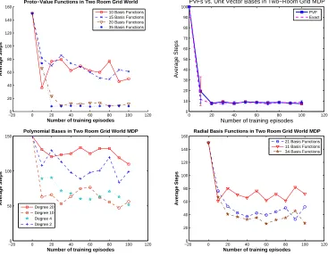
Number of Basis Functions: Figure 9 evaluates the learned policy by measuring the number of steps to reach the goal, as a function of the number of training episodes, and as the number of basis functions is varied (ranging from 10 to 35 for each of the four actions). The results are averaged over 10 independent runs, where each run consisted of a set of training episodes of a maximum length of 100 steps, where each episode was terminated if the agent reached the absorbing goal state. Around 20 basis functions (per action) were sufficient to get close to optimal behavior, and increasing the number of bases to 35 produced a marginal improvement. The variance across runs is fairly small for 20 and 35 bases, but relatively large for smaller numbers of bases (not shown for clarity). Figure 9 also compares the performance of PVFs with unit vector bases (table lookup), showing that PVFs with 25 bases closely tracks the performance of unit vector bases on this task. Note that we are measuring performance in terms of the number of steps to reach the goal, averaged over a set of 10 runs. Other metrics could be plotted as well, such as the total discounted reward received, which may be more natural. However, our point is simply to show that there are significant differences in the quality of the policy learned by PVFs with that learned by the other parametric approximators, and these differences are of such an order that they will clearly manifest themselves regardless of the metric used.

Comparison with Parametric Bases: One important consideration in evaluating PVFs is how they compare with standard parametric bases, such as radial basis functions and polynomials. As Figure 1 suggests, parametric bases as conventionally formulated may have difficulty representing highly nonlinear value functions in MDPs such as the two room task. Here, we test whether this poor performance can be ameliorated by varying the number of basis functions used. Figure 9 evaluates the effectiveness of polynomial bases and radial basis functions in the two room MDP. In polynomial bases, a state i is mapped to the vectorφ(i) = (1,i,i2, . . .ik−1)for k basis functions—this architecture was studied by (Koller and Parr, 2000; Lagoudakis and Parr, 2003).12In RBFs, a state i 11. In Section 9, we describe more sophisticated diffusion models for grid-world tasks in the richer setting of semi-Markov decision processes (SMDPs), using directed state-action graphs with temporally extended actions, such as “exiting a room”, modeled with distal edges (Osentoski and Mahadevan, 2007).