A Nonparametric Statistical Approach to Clustering via Mode
Identification
Jia Li [email protected]
Department of Statistics
The Pennsylvania State University University Park, PA 16802, USA
Surajit Ray [email protected]
Department of Mathematics and Statistics Boston University
Boston, MA 02215, USA
Bruce G. Lindsay [email protected]
Department of Statistics
The Pennsylvania State University University Park, PA 16802, USA
Editor: Charles Elkan
Abstract
A new clustering approach based on mode identification is developed by applying new optimiza-tion techniques to a nonparametric density estimator. A cluster is formed by those sample points that ascend to the same local maximum (mode) of the density function. The path from a point to its associated mode is efficiently solved by an EM-style algorithm, namely, the Modal EM (MEM). This method is then extended for hierarchical clustering by recursively locating modes of kernel density estimators with increasing bandwidths. Without model fitting, the mode-based clustering yields a density description for every cluster, a major advantage of mixture-model-based clustering. Moreover, it ensures that every cluster corresponds to a bump of the density. The issue of diagnos-ing clusterdiagnos-ing results is also investigated. Specifically, a pairwise separability measure for clusters is defined using the ridgeline between the density bumps of two clusters. The ridgeline is solved for by the Ridgeline EM (REM) algorithm, an extension of MEM. Based upon this new measure, a cluster merging procedure is created to enforce strong separation. Experiments on simulated and real data demonstrate that the mode-based clustering approach tends to combine the strengths of linkage and mixture-model-based clustering. In addition, the approach is robust in high dimensions and when clusters deviate substantially from Gaussian distributions. Both of these cases pose diffi-culty for parametric mixture modeling. A C package on the new algorithms is developed for public access at http://www.stat.psu.edu/∼jiali/hmac.
Keywords: modal clustering, mode-based clustering, mixture modeling, modal EM, ridgeline
EM, nonparametric density
1. Introduction
is applied to text documents or images to speed up indexing and retrieval (Li, 2005a). Clustering can be a stand-alone process. For example, microarray gene expression data are often clustered in order to find genes with similar functions. Clustering is also the technical core of several prototype-based supervised learning algorithms (Hastie et al., 2001) and has been extended to non-vector data in this regard (Li and Wang, 2006). Recent surveys (Kettenring, 2006; Jain et al., 1999) discuss the methodologies, practices, and applications of clustering.
1.1 Background
Clustering methods fall roughly into three types. The first type uses only pairwise distances between objects to be clustered. These methods enjoy wide applicability since a tractable mathematical representation for objects is not required. However, they do not scale well with large data sets due to the quadratic computational complexity of calculating all the pairwise distances. Examples include linkage clustering (Gower and Ross, 1969) and spectral graph partitioning (Pothen et al., 1990). The second type targets on optimizing a given merit function. The merit function reflects the general belief about good clustering, that is, objects in the same cluster should be similar to each other while those in different clusters be as distinct as possible. Different algorithms vary in the similarity measure and the criterion for assessing the global quality of clustering. K-means and k-center clustering (Gonzalez, 1985) belong to this type.
The third type relies on statistical modeling (Fraley and Raftery, 2002). In particular, each cluster is characterized by a basic parametric distribution (referred to as a component), for instance, the multivariate Gaussian for continuous data and the Poisson distribution for discrete data. The overall probability density function (pdf) is a mixture of the parametric distributions (McLachlan and Peel, 2000). The clustering procedure involves first fitting a mixture model, usually by the EM algorithm, and then computing the posterior probability of each mixture component given a data point. The component possessing the largest posterior probability is chosen for that point. Points associated with the same component form one cluster. Moreover, the component posterior probabilities evaluated in mixture modeling can be readily used as a soft clustering scheme. In addition to partitioning data, a probability distribution is obtained for each cluster, which can be helpful for gaining insight into the data. Another advantage of mixture modeling is its flexibility in treating data of different characteristics. For particular applications, mixtures of distributions other than Gaussian have been explored for clustering (Banfield and Raftery, 1993; Li and Zha, 2006). Banerjee et al. (2005) have also used the mixture of Mises-Fisher distributions to cluster data on a unit sphere.
The advantages of mixture modeling naturally result from its statistical basis. However, the parametric assumptions about cluster distributions are found restrictive in some applications. Li (2005b) addresses the problem by assuming each cluster itself is a mixture of Gaussians, providing greater flexibility for modeling a single cluster. This method involves selecting the number of components for each cluster and is sensitive to initialization. Although some success has been shown using the Bayesian Information Criterion (BIC), choosing the right number of components for a mixture model is known to be difficult, especially for high dimensional data.
“hilltop”, that is, the mode. The rational for clustering by a mixture model is that if the component distributions each possess a single hilltop, by fitting a mixture of them, every component captures one separate hilltop in the data. However, this is often not true. Without careful placement and control of their shapes, the mixture components may not align with the hills of the density, especially when clusters are poorly separated or the assumed parametric component distribution is violated. It is known that two Gaussians located sufficiently close result in a single mode. (On the other hand, a two component multivariate Gaussian mixture can have more than two modes, as shown by Ray and Lindsay, 2005). In this case, equating a component with a cluster is questionable. This profound limitation of mixture modeling has not been adequately investigated. In fact, even to quantify the separation between components is not easy.
Here, we develop a new nonparametric clustering approach, still under a statistical framework. This approach inherits the aforementioned advantages of mixture modeling. Furthermore, data are allowed to reveal a nonparametric distribution for each cluster as part of the clustering procedure. It is also guaranteed that every cluster accounts for a distinct hill of the probability density.
1.2 Clustering via Mode Identification
To avoid restrictions imposed by parametric assumptions, we model data using kernel density func-tions. By their nature, such densities have a mixture structure. Given a density estimate in the form of a mixture, a new algorithm, aptly called the Modal EM (MEM), enables us to find an increasing path from any point to a local maximum of the density, that is, a hilltop. Our new clustering algo-rithm groups data points into one cluster if they are associated with the same hilltop. We call this approach modal clustering. A new algorithm, namely the Ridgeline EM (REM), is also developed to find the ridgeline linking two hilltops, which is proven to pass through all the critical points of the mixture density of the two hills.
The MEM and REM algorithms allow us to exploit the geometry of a probability density func-tion in a nontrivial manner. As a result, clustering can be conducted in accurate accordance with our geometric heuristics. Specifically, every cluster is ensured to be associated with a hill, and ev-ery sample point in the cluster can be moved to the corresponding hilltop along an ascending path without crossing any “valley” that separates two hills. Moreover, by finding the ridgeline between two hilltops, the way two hills separate from each other can be adequately measured and exhibited, enabling diagnosis of clustering results and application-dependent adjustment of clusters. Modal clustering using MEM also has practical advantages such as the irrelevance of initialization and the ease of implementing required optimization techniques.
Our modal clustering algorithm is not restricted to kernel density estimators. In fact, it can be used to find the modes of any density in the form of a mixture distribution. It is known that when the number of components in a mixture increases, as long as there are sufficiently many components, the overall fitted density of the mixture is not sensitive to that number. On the other hand, the resulting partition of data can change dramatically if we identify each mixture component with a cluster, as normally practiced in mixture-model-based clustering. In modal clustering, there is no such identification, and mixture components only play the role of approximating a density. We thus have much more flexibility at choosing mixture distributions. Specifically, we adopt the fully nonparametric kernel density estimation, using Gaussian kernels for continuous data.
• A new nonparametric statistical clustering algorithm and its hierarchical extension are devel-oped by associating data points to their modes identified by MEM. Approaches to improve computational efficiency and to visualize cluster structures for high dimensional data are pre-sented.
• The REM algorithm is developed to find the ridgeline between the modes of any two clusters. Measures for the pairwise separability between clusters are proposed using ridgelines. A cluster merging algorithm to enhance modal clustering is developed.
• Experiments are conducted using both simulated and real data sets. Comparisons are made with several other clustering algorithms such as linkage clustering, k-means, and Gaussian mixture modeling.
1.3 Related Work
Clustering is an extensively studied research topic with vast existing literature (see Jain et al., 1999; Everitt et al., 2001, for general coverage). Works most related to ours are mode-based clustering methods independently developed in the communities of pattern recognition (Leung et al., 2000) and statistics (Cheng et al., 2004). The MEM and REM algorithms, the cluster diagnosis tool, and cluster merging procedure built upon REM are unique to our work.
In pattern recognition, mode-based clustering is studied under the name of scale-space method, inspired by the smoothing effect of the human visual system. The scale-space clustering method is pioneered by Wilson and Spann (1990), and furthered studied by Roberts (1997) using density estimation and by Chakravarthy and Ghosh (1996) using the radial basis function neural network. Leung et al. (2000) forms a function called “space scale image” for a data set. This function is es-sentially a Gaussian kernel density estimate (differing from a true density by an ignorable constant). The modes of the density function are solved by numerical methods. To associate a data point with a mode, a gradient dynamic system starting from the point is defined and solved by the Euler differ-ence method. A hierarchical clustering algorithm is proposed by gradually increasing the Gaussian kernel bandwidth. The authors also note the non-nested nature of clustering results obtained from increasing bandwidths.
It can be shown that the iteration equation derived from the Euler difference method is identi-cal to that from MEM. However, MEM applies generally to any mixture of Gaussians as well as mixtures of other parametric distributions. Its ascending property is proved rather than based on approximation. Under the framework of scale-space clustering, general mixtures do not arise as a concern, and naturally, only the case of Gaussian kernel density is discussed (Leung et al., 2000). It is not clear whether the gradient dynamic system can be efficiently solved for general mixture models. Our hierarchical clustering algorithm differs slightly from that of Leung et al. (2000) by enforcing nested clustering. This difference only reflects an algorithmic preference and is not in-trinsic to the key ideas of modal clustering.
relationship between kernel bandwidths and the modes of uni- or bivariate kernel density functions. Minnotte et al. (1998) also extended the mode tree to the mode forest.
Because clustering of independent vectors has been a widely used method for image segmen-tation, especially in the early days (Jain and Dubes, 1988), we test the efficiency of our algorithm on segmentation, a good example of computationally intensive applications. We have no intention to present our clustering algorithm as a state-of-the-art segmentation method although it may well be applied as a fast method. We note that much advance has been achieved in image segmentation using approaches beyond the framework of clustering independent vectors (Pal and Pal, 1993; Shi and Malik, 2000; Joshi et al., 2006).
The rest of the paper is organized as follows. Notations and the MEM algorithm are introduced in Section 2. In Section 3, a new clustering algorithm and its hierarchical extension are developed by associating data points with the modes of a kernel density estimate. In Section 4, the REM algo-rithm for finding ridgelines between modes is presented. In addition, several measures of pairwise separability between clusters are defined, which lead to the derivation of a new cluster merging algorithm. This merging method strengthens the framework of modal clustering. In Section 5, we present a method to visualize high dimensional data so that the discrimination between clusters is well preserved. Experimental results on both simulated and real data sets and comparisons with other clustering approaches are provided in Section 6. Finally, we conclude and discuss future work in Section 7.
2. Preliminaries
We introduce in this section the Modal EM (MEM) algorithm that solves a local maximum of a mixture density by ascending iterations starting from any initial point. The algorithm is named Modal EM because it comprises two iterative steps similar to the expectation and the maximization steps in EM (Dempster et al., 1977). The objective of the MEM algorithm is different from the EM algorithm. The EM algorithm aims at maximizing the likelihood of data over the parameters of an assumed distribution. The goal of MEM is to find the local maxima, that is, modes, of a given distribution.
Let a mixture density be f(x) =∑Kk=1πkfk(x), where x∈
R
d, πk is the prior probability ofmixture component k, and fk(x)is the density of component k. Given any initial value x(0), MEM
solves a local maximum of the mixture by alternating the following two steps until a stopping criterion is met. Start with r=0.
1. Let
pk=πk
fk(x(r))
f(x(r)) ,k=1, ...,K.
2. Update
x(r+1)=argmax
x K
∑
k=1pklog fk(x).
The first step is the “Expectation” step where the posterior probability of each mixture com-ponent k, 1≤k≤K, at the current point x(r) is computed. The second step is the “Maximiza-tion” step. We assume that∑Kk=1pklog fk(x)has a unique maximum, which is true when the fk(x)
x(r+1)=∑K
k=1pkµk. For other parametric densities fk(x), the solution to the maximization in the
second step can be more complicated and sometimes requires numerical procedures. On the other hand, similarly as in the EM algorithm, it is usually much easier to maximize∑Kk=1pklog fk(x)than
the original objective function log∑Kk=1πkfk(x).
The proof of the ascending property of the MEM algorithm is provided in Appendix A. We omit a rigorous discussion regarding the convergence of x(r)here. By Theorem 1 of Wu (1983), if f(x) is a mixture of normal densities, all the limit points of {x(r)} are stationary points of f(x). It is possible that{x(r)}converges to a stationary, but not locally maximal, point, although we have not observed this in our experiments. We refer to (Wu, 1983) for a detailed treatment of the convergence properties of EM style algorithms.
3. Clustering by Mode Identification
We focus on clustering continuous vector data although the framework extends readily to discrete data. Given a data set{x1,x2, ...,xn}, xi∈
R
d, a probability density function for the data is estimatednonparametrically using Gaussian kernels. As the kernel density estimate is in the form of a mixture distribution, MEM is applied to find a mode using every sample point xi, i=1, ...,n, as the initial
value for the iteration. Two points xiand xjare grouped into one cluster if the same mode is obtained
from both. When the variances of Gaussian kernels increase, the density estimate becomes smoother and tends to group more points into one cluster. A hierarchy of clusters can thus be constructed by gradually increasing the variances of Gaussian kernels. Next, we elaborate upon the clustering algorithm, illustrate it with an example, and discuss approaches to speed up computation.
3.1 The Algorithm
Let the set of data to be clustered be S={x1,x2, ...,xn}, xi ∈
R
d. The Gaussian kernel densityestimate is formed:
f(x) =
n
∑
i=1 1nφ(x|xi,Σ),
where the Gaussian density function
φ(x|xi,Σ) =
1
(2π)d/2|Σ|1/2exp(− 1 2(x−xi)
tΣ−1(x−x
i)).
We use a spherical covariance matrix Σ=diag(σ2,σ2, ...,σ2). The standard deviation σ is also referred to as the bandwidth of the Gaussian kernel. We use notation D(σ2) =diag(σ2,σ2, ...,σ2) for brevity.
With a given Gaussian kernel covariance matrix D(σ2), data are clustered as follows: 1. Form kernel density
f(x|S,σ2) =
n
∑
i=1 1nφ(x|xi,D(σ
2)), (1)
2. Use f(x|S,σ2) as the density function. Use each x
i, i=1,2, ...,n, as the initial value in the
MEM algorithm to find a mode of f(x|S,σ2). Let the mode identified by starting from x
i be
3. Extract distinctive values from the set {
M
σ(xi),i=1,2, ...,n} to form a set G. Label theelements in G from 1 to|G|. In practice, due to finite precision, two modes are regarded equal if their distance is below a threshold.
4. If
M
σ(xi)equals the kth element in G, xiis put in the kth cluster.In the basic version of the algorithm, the density f(x|S,σ2)is a sum of Gaussian kernels centered at every data point. However, the algorithm can be carried out with any density estimate in the form of a mixture. The key step in the clustering algorithm is the identification of a mode starting from any xi. MEM moves from xi via an ascending path, or, figuratively, via hill climbing, to a mode.
Points that climb to the same mode are located on the same hill and hence grouped into one cluster. We call this the Mode Association Clustering (MAC) algorithm.
Although the density of each cluster is not explicitly modeled by MAC, this nonparametric method retains a major advantage of mixture-model-based clustering, that is, a pdf is obtained for each cluster. These density functions facilitate soft clustering as well as cluster assignment of samples outside the data set. Denote the set of points in cluster k, 1≤k≤ |G|, by Ck. The density
estimate for cluster k is
gk(x) =
∑
xi:xi∈Ck1
|Ck|
φ(x|xi,D(σ2)). (2)
Because we do not assume a parametric form for the densities of individual clusters, our method tends to be more robust and characterizes clusters more accurately when the attempted parametric assumptions are violated.
It is known in the literature of mixture modeling that if the density of a cluster is estimated using only points assigned to this cluster, the variance tends to be under estimated, although the effect on clustering may be small (Celeux and Govaert, 1993). The under estimation of variance becomes more severe for poorly separated clusters, which often decay towards zero too quickly on leaving the cluster. We will see a similar phenomenon here with gk(x) having over fast decaying tails. A
correction to this problem in mixture modeling is to use soft instead of hard clustering. Every point is allowed to contribute to every cluster by a weight computed from the posterior probability of the cluster.
Under this spirit, we can make an ad-hoc modification on the density estimation. With gk(x)in
(2) as the initial cluster density, compute the posterior of cluster k given each xiby pi,k∝|Cnk|gk(x),
k=1, ...,|G|, subject to∑k|G0=|1pi,k0 =1. Form the updated density of cluster k by
˜
gk(x) =∑ n
i=1pi,kφ(x|xi,D(σ2))
∑n i=1pi,k
.
With the cluster density modified, it is natural to question if pi,k should be updated again, which
in turn will lead to another update of ˜gk(x). This iterative procedure can be carried out infinitely.
Whether it converges is not clear and may be worthy of investigation. On the other hand, if the maximum a posteriori clustering based on the final ˜gk(x) differs significantly from the result of
modal clustering, this procedure may have defeated the very purpose of modal clustering and turned it into merely an initialization scheme. We thus do not recommend many iterative updates on ˜gk(x).
One round of adjustment from gk(x)may be sufficient. Or one can take gk(x)cautiously as a smooth
When the bandwidthσincreases, the kernel density estimate f(x|S,σ2)in (1) becomes smoother and more points tend to climb to the same mode. This suggests a natural approach for hierarchical clustering. Given a sequence of bandwidthsσ1<σ2<· · ·<ση, hierarchical clustering is performed in a bottom-up manner. We start with every point xi being a cluster by itself. The set of cluster
representatives is thus G0=S={x1, ...,xn}. This extreme case corresponds to the limit when σ
approaches 0. At any bandwidthσl, the cluster representatives in Gl−1obtained from the preceding bandwidth are input into MAC using the density f(x|S,σ2
l). Note that the kernel centers remain
at all the original data points although modes are identified only for cluster representatives when l>1. The modes identified at this level form a new set of cluster representatives Gl. This procedure
is repeated across allσl’s. We refer to this hierarchical clustering algorithm as Hierarchical MAC
(HMAC). It corresponds to the mappings xi→
M
σ1(xi)→M
σ2(M
σ1(xi))→ · · ·.Denote the partition of points obtained at bandwidthσlby
P
l, a function mapping xi’s to clusterlabels. If K clusters labeled 1, 2, ..., K, are formed at bandwidthσl,
P
l(xi)∈ {1,2, ...,K}. HMACensures that
P
l’s are nested, that is, ifP
l(xi) =P
l(xj), thenP
l+1(xi) =P
l+1(xj). Recall that theset of cluster representatives at level l is Gl. HMAC starts with G0 ={x1, ...,xn} and solves Gl,
l=1,2, ...,η, sequentially by the following procedure:
1. Form kernel density
f(x|S,σ2l) =
n
∑
i=1 1nφ(x|xi,D(σ 2
l)).
2. Cluster Gl−1by MAC using density f(x|S,σ2l). Let the set of distinct modes obtained be Gl.
3. If
P
l−1(xi) =k and the kth element in Gl−1is clustered to the k0th mode in Gl, thenP
l(xi) =k0.That is, the cluster of xiat level l is determined by its cluster representative in Gl−1.
It is worthy to note that HMAC differs profoundly from linkage clustering, which also builds a hierarchy of clusters. In linkage clustering, at every level, only the two clusters with the minimum pairwise distance are merged. The hierarchy is constructed by a sequence of such small greedy merges. The lack of overall consideration tends to result in skewed clusters. In HMAC, however, at any level, the merging of clusters is conducted globally and the effect of every original data point on clustering is retained through the density f(x|S,σ2
l).
3.2 An Example
We now illustrate the HMAC algorithm using a real data set. This is the glass identification data provided by the UCI machine learning database repository (Blake et al., 1998). The original data were contributed by Spiehler and German at the Diagnostic Products Corporation. For clarity of demonstration, we take 105 sample points from two types of glass in this data set. Moreover, we only use the first two principal components of the original 9 dimensions.
HMAC is applied to the data using a sequence of kernel bandwidthsσ1<σ2<· · ·<ση,η=20, chosen equally spaced from [0.1 ˆσ,2 ˆσ] = [0.225,4.492], where ˆσ is the larger one of the sample standard deviations of the two dimensions. Among the 20 differentσl’s, only 6 of them result in
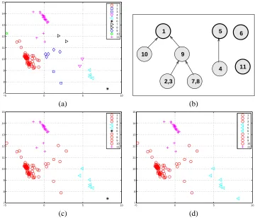
We demonstrate the clustering results at the 2nd and 3rd level in Figure 1. At the 2nd level, 11 clusters are formed, as shown by different symbols in Figure 1(a). The 11 modes identified at level 2 are merged into 5 modes at level 3 when the bandwidth increases from 0.449 to 0.674. Figure 1(b) shows the ascending paths generated by MEM from the 11 modes (crosses) at level 2 to the 5 modes (squares) at level 3. The contour lines of the density function with the corresponding bandwidth of level 3 are plotted in the background for better illustration. The 5 clusters at level 3 are shown in Figure 1(c). These 5 modes are again merged into 3 modes at level 4, as shown in Figure 1(d).
3.3 Measures for Enhancing Speed
Because the nonparametric density estimate in (1) is a sum of kernels centered at every data point, the amount of computation to identify the mode associated with a single point grows linearly with n, the size of the data set. The computational complexity of clustering all the data by MAC is thus quadratic in n. In practice, however, it is often unnecessary to use the basic kernel estimate. A preliminary clustering can be first applied to{x1, ...,xn}to yield m clusters, where m is significantly
smaller than n, but still much larger than the desired number of clusters. Suppose the m cluster centroids are S={x1, ...,xm}and the number of points in cluster Sj is nj, j=1,2, ...,m. We use the
density estimate
f(x|S,D(σ2)) =
m
∑
j=1nj
nφ(x|xj,D(σ 2))
in MAC to cluster the xi’s. Since MEM applies to general mixture models, the modified density
function causes no essential changes to the clustering procedure.
The purpose of the preliminary clustering is more of quantizing the data than clustering. Com-putation is reduced by not discerning points in the same quantization region when formulating the density estimate. If m is sufficiently large, S is adequate to retain the topological structures in the nonparametric density estimate. In this fast version of MAC, we search for a mode for every xi.
Examples exploiting the fast MAC are given in Section 6.
4. Analysis of Cluster Separability via Ridgelines
A measure for the separability between clusters is useful for gaining deeper understanding of clus-tering structures in data. With this measure, the difference between clusters is quantified, rather than being simply categorical. This quantification can be useful in certain situations. For instance, in taxonomy study, after grouping instances into species, scientists may need to numerically assess the disparity between species, often taken as an indicator for evolutionary proximity. A separability measure between the clusters of species can effectively reflect such disparity. Such a measure is also useful for diagnosing clustering results and for the mere interest of designing clustering algorithms. Based upon it, we derive a mechanism to merge weakly separated clusters. Although the separabil-ity measure is a diagnostic tool and the cluster merging method can adjust the number of clusters, in this paper, we do not pursue the problem of choosing the number of clusters fully automatically. It is well known that determining this number is a deep problem, and domain knowledge often needs to be called upon for a final decision in various applications.
−5 0 5 10 7 8 9 10 11 12 13 14 15 1 2 3 4 5 6 7 8 9 10 11
−5 0 5 10
7 8 9 10 11 12 13 14 15 (a) (b)
−5 0 5 10
7 8 9 10 11 12 13 14 15 1 2 3 4 5
−5 0 5 10
7 8 9 10 11 12 13 14 15 (c) (d)
−5 0 5 10
7 8 9 10 11 12 13 14 15
0 0.2 0.4 0.6 0.8 1 0
0.5 1
Ridgeline density (scaled) 0 0.2 0.4 0.6 0.8 1
0 0.5 1
0 0.2 0.4 0.6 0.8 1 0
0.5 1
α
(e) (f)
define a ridgeline between two unimodal clusters. The REM algorithm is developed to solve the ridgeline.
4.1 Ridgeline
The ridgeline between two clusters with density g1(x)and g2(x)is
L
={x(α):(1−α)∇log g1(x) +α∇log g2(x) =0,0≤α≤1}. (3)For a mixture density of the two clusters, ˜g(x) =π1g1(x) +π2g2(x),π1+π2=1, if ˜g(x)>0 for any x, the modes, antimodes (local minimums), and saddle points of ˜g(x) must occur in
L
for any prior probabilityπ1. The locations of these critical points, however, depend onπ1. This fact is referred to as the critical value theorem and is proved by Ray and Lindsay (2005).Remarks:
1. Eq. (3) is precisely the critical point equation for the exponential tilt density g(x|α) = c(α)g1(x)1−αg2(x)α, where c(α) is a normalizing constant. This density family is an
ex-ponential family, with sufficient statistic log(g2(x)/g1(x)).
2. The set of solutions in
L
is, in general, a 1-dimensional manifold; that is, a curve. When both g1and g2are normal densities, the solution is explicit (see Ray and Lindsay, 2005), and the solutions form a unique one-dimensional curve. More generally, the solutions are possibly a set of curves that pass through the modes of the g1(x)and g2(x).3. If both g1and g2are unimodal and have convex upper contour sets, it can be proved that the solutions form a unique curve between the modes of g1and g2respectively. In our discussion, we assume unimodal g1and g2.
Since the local maxima of the exponential tilt function g(x;α)satisfy Eq. (3), we solve (3) by maximizing log(g(x|α)) = (1−α)log g1(x) +αlog g2(x). In the case when the two cluster densi-ties g1 and g2are themselves mixtures of basic parametric distributions, for example, normal, we develop an ascending algorithm to maximize the function, referred to as the Ridgeline EM (REM) Algorithm. For notational brevity, assume that both g1 and g2 are mixtures of T parametric distri-butions:
gi(x) = T
∑
κ=1
πi,κhi,κ(x), i=1,2.
Starting from an initial value x(0), REM updates x by iterating the two steps: 1. Compute
pi,κ=πi,κhi,κ(x(r))/
T
∑
j=1πi,jhi,j(x(r)), κ=1, ...,T,i=1,2.
2. Update x(r+1):
x(r+1)=argmax
x
(1−α)
T
∑
κ=1
p1,κlog h1,κ(x) +α
T
∑
κ=1
REM ensures that g(x(r+1)|α)≥g(x(r)|α). Proof is given in Appendix B. As with MEM, we will not rigorously study the convergence properties of the sequence{x(r)}. In the special case hi,κ(x) =φ(x|µi,κ,Σ), the update equation for x(r+1)becomes
x(r+1)= (1−α)
T
∑
κ=1
p1,κµ1,κ+α
T
∑
κ=1
p2,κµ2,κ.
The Gaussian kernel density estimate belongs to this case.
At the two extreme valuesα=0,1, the solutions are the modes of g1(x)and g2(x)respectively. We solve x(α) sequentially on a set of grid points 0=α0 <α1<· · ·<αζ=1. First, x(0) = argmaxxg1(x) is solved by MEM. For every αl, x(αl−1), previously calculated, is used as initial value to start the iterations in REM.
Suppose two clusters, denoted by z1and z2, have densities g1and g2, and prior probabilitiesπ1 andπ2respectively. We define a pairwise separability as
S(z1,z2) =1−
minαπ1g1(x(α)) +π2g2(x(α)) π1g1(x(0)) +π2g2(x(0)) =1−
π1g1(x(α∗)) +π2g2(x(α∗))
π1g1(x(0)) +π2g2(x(0)) (4) whereα∗=argminαπ1g1(x(α)) +π2g2(x(α)). Usually, the prior probabilitiesπ1orπ2are propor-tional to the cluster sizes. It is obvious that S(z1,z2)∈[0,1]. To symmetrize the measure, we define the pairwise symmetric separability as ˜S(z1,z2) =min[S(z1,z2),S(z2,z1)].
By finding x(α∗), we can evaluate the amount of “dip” along the ridgeline. By the critical value theorem, the minimum of π1g1(x) +π2g2(x), if exists, lies on the ridgeline and therefore must be x(α∗). Hence, if there is a “dip” in the mixture of the two clusters, it will be captured by the ridgeline. According to definition (4), a deeper “dip” leads to higher separability. In our implementation, we approximateα∗by
α∗≈argmin
αl,0≤l≤ζ
π1g1(x(αl)) +π2g2(x(αl)),
whereαl, 0≤l≤ζ, are the grid points.
We also define the separability for a single cluster to quantify its overall distinctness from other clusters. Specifically, suppose there are m clusters denoted by zi, i=1, ...,m. The separability of
cluster zi, denoted by s(zi)is defined by
s(zi) = min
j:1≤j≤m,j=6 iS(zi,zj).
We call a cluster “insignificant” if its separability is below a given thresholdε. In our discussion, ε=0.5.
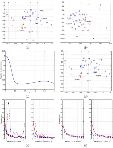
Take the glass data set as an example. As shown in Figure 1(c), the points are divided into 5 groups at that level of the clustering hierarchy. Two of the clusters each contain a single sample point, which is far from the other points and forms a mode alone. The separability of these two clusters are weak, respectively 0.00 and 0.30. The three other clusters are highly separable, with separability values 0.94, 0.84 and 0.81. Figure 1(e) shows the ridgelines between any two of the three significant clusters, and Figure 1(f) shows the density function along the ridgelines, normalized to one at the ridgeline end point x(0)or x(1)(depending on whichever is larger).
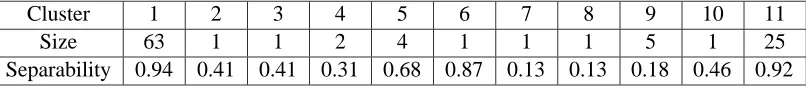
is not the sole factor affecting separability. Take the clusters in Figure 1(a) as an example. The separability of the 11 clusters and their corresponding sizes (number of points contained) are listed in Table 1. It is shown that although cluster 9 is the third largest cluster, its separability is low. At thresholdε=0.5, this cluster is insignificant. In contrast, by being far from all the other clusters, cluster 6, a singleton, has separability 0.87. The low separability of cluster 9 is caused by its prox-imity to cluster 1, the largest cluster which accounts for 60% of the data. Clusters that contain a large portion of data tend to “absorb” surrounding smaller clusters. The attraction of a small cluster to a bigger one depends on its relative size, tightness, distance to the bigger cluster, as well as the orientation of the data masses in the two clusters.
Cluster 1 2 3 4 5 6 7 8 9 10 11
Size 63 1 1 2 4 1 1 1 5 1 25
Separability 0.94 0.41 0.41 0.31 0.68 0.87 0.13 0.13 0.18 0.46 0.92
Table 1: Separability between clusters in the glass data set
4.2 Merging Clusters Based on Separability
To elaborate on the relationships between clusters, we compute the matrix of separability between any pair of clusters. We can potentially use this matrix to decide which clusters can be merged due to weak separation. As discussed previously, one way to merge clusters is to increase the bandwidth of the kernel function used by HMAC. However, an enlarged bandwidth may cause prominent clus-ters to be clumped while leaving undesirable small “noisy” clusclus-ters unchanged. Merging clusclus-ters according to the separability measure is one possible approach to eliminate “noisy” clusters without losing important clustering structures found at a small bandwidth. We will show by the glass data that the merging method makes clustering results less sensitive to bandwidth.
Let the clusters in consideration be{z1,z2, ...,zm}. We denote the pairwise separability between
cluster ziand zjin short by Si,j, where Si,j=S(zi,zj). Note in general Si,j6=Sj,i. Let a threshold for
separability beε, 0<ε<1. Let the density function of cluster zi be gi(·)and the prior probability
beπi. Denote the weighted mode of each cluster density function byδ(zi) =πimax gi(x). Since in
MEM the mode max gi(x)for each cluster ziis computed when ziis formed,δ(zi)requires no extra
computation after clustering. We refer toδ(zi)as the significance index of cluster zi.
The main idea of the merging algorithm is to have clusters with a higher significance index absorb other clusters that are not well separated from them and are less dominant (lower significance index). Several issues need to be resolved to avoid arbitrariness in merging. First, a cluster zimay be
weakly separated from several other clusters with higher significance indices. Among those clusters, we let the one from which ziis worst separated to absorb zi. Second, two weakly separated clusters
zi and zj may have the same significance indices, that is,δ(zi) =δ(zj); and hence it is ambiguous
which cluster should be treated as the dominant one. We solve this problem by introducing the concept of cliques. The clusters are first grouped into cliques which contain weakly separated zi’s
with the same value ofδ(zi). Clusters in different cliques are ensured to be either well separated or
Next, we describe how to form cliques and extend the definition of pairwise separability to cliques. In order to carry out the merging of cliques, a directed graph is constructed upon the cliques based on pairwise separability and the comparison of significance indices.
1. Tied: Cluster zi and zjare defined to be tied if S(zi,zj)<εandδ(zi) =δ(zj).
2. Clique: Cluster ziand zj are in the same clique if (a) ziand zjare tied, or (b) there is a cluster
zk such that ziand zkare in the same clique, and zj and zkare in the same clique.
Remark: the relationship “tied” results in a partition of zi’s. Each group formed by the
par-tition is a clique. Because being tied requiresδ(zi) =δ(zj), in practice, we only observe
clusters being tied when they are all singletons.
We now define the separability between cliques. Without loss of generality, let clique c1=
{z1,z2, ...,zm1}and c2={zm1+1, ...,zm1+m2}. Denote the clique-wise separability by Sc(c1,c2):
Sc(c1,c2), min
1≤i≤m1
min
m1+1≤j≤m1+m2
S(zi,zj).
Since in general, S(zi,zj)6=S(zj,zi), the asymmetry carries over to Sc(c1,c2)6=Sc(c2,c1). We also denote the significance index of a clique ci asδ(ci). Since all the clusters in ci have equal
significance indices, we letδ(ci) =δ(zi0), where zi0 is any cluster included in ci.
Regard each clique as a node in a graph. Suppose there are ˜m cliques{c1, ...,cm˜}. A directed graph is built as follows. For two arbitrary cliques ciand cj, a link from ci to cj is made if
1. Sc(ci,cj)<ε.
2. Sc(ci,cj) =mink6=iSc(ci,ck) and j is the smallest index among all those j0’s that achieve
Sc(ci,cj0) =mink6=iSc(ci,ck).
3. δ(ci)<δ(cj).
A clique ci is said to be linked to cj if there is a directed edge from ci to cj. It is obvious by
the second requirement in the link construction that every clique is linked to at most another clique. In Appendix C, it is proved that a graph built by the above rules has no loops. An example graph is illustrated in Figure 2(b). If we disregard the directions of the links, the graph is partitioned into connected subgraphs. In the given example in Figure 2(b), there are four connected subgraphs. The basic idea of the merging algorithm is to let the most dominant clique in one subgraph absorb all the others in the same subgraph.
We call clique cj the parent clique of ci if there is a directed link from cito cj. In this case, we
also say ciis directly absorbed by cj. By construction,δ(ci)<δ(cj). More generally, if there is a
directed path from cito cj, then cj is called an ancestor of ci, and ci is absorbed by cj. Again, we
have δ(ci)<δ(cj)by transitivity. In each connected subgraph containing k nodes, because there
than that of any other clique in the subgraph. In this sense, the head clique dominates all the other connected cliques.
Combining clusters by the above method is the first and main step in our merging algorithm. To account for outliers, the second step in the algorithm employs the notation of coverage rate. Outlier points far from all the essential clusters tend to yield high separability and hence will not be merged. In HMAC, to “grab” those outliers, the kernel bandwidth needs to grow so large that under such a bandwidth, many significant clusters are undesirably merged. To address this issue, we find the smallest clusters and mark them as outliers if their total size proportional to the entire data set is below a threshold. For instance, if the coverage rate allowed is 95%, this threshold is then 5%.
We now summarize our cluster merging algorithm as follows. We call the merging procedure conducted based on the separability measure stage I merging and that based on coverage rate stage II merging. The two stages do not always have to be concatenated. We can apply each alone. Applying only stage I is equivalent to applying two stages and setting the coverage rate to 100%; applying only stage II is equivalent to setting the threshold of separability to 0.0. Assume the starting clusters
are{z1,z2, ...,zm}.
1. Stage I: merging based on separability.
(a) Compute the separability matrix [Si,j], i,j=1, ...,m, and the significant index δ(zi),
i=1, ...,m.
(b) Form cliques{c1,c2, ...,cm˜}based on[Si,j]andδ(zi)’s, where ˜m≤m. Record the zi’s
contained in each clique.
(c) Construct the directed graph.
(d) Merge cliques that are in the same connected subgraph. zi’s contained in merged cliques
are grouped into one cluster. Denote those merged clusters by {ˆz1,ˆz2, ...,ˆzmˆ}, where ˆ
m≤m.˜
2. Stage II: merging based on coverage rate. Denote the coverage rate byρ.
(a) Calculate the sizes of clusters{ˆz1,ˆz2, ...,ˆzmˆ}and denote them by ˆni, i=1, ...,m. Theˆ
size of the whole data set is n=∑mˆ
i=1nˆi.
(b) Sort ˆni, i=1, ...,m, in ascending order. Let the sorted sequence be ˆˆ n(1), ˆn(2), ..., ˆn(mˆ). Let ˆn(0)=0. Let k be the largest integer such that∑ki=0nˆ(i)≤(1−ρ)n.
(c) If k>0, go to the next step. Otherwise, stop and the final clusters are{ˆz1,ˆz2, ...,ˆzmˆ}. (d) For each ˆz(i), i=1, ...,k, find all the original clusters zj’s that are merged into ˆz(i). Denote
the index set of the zj’s by H(i). Let H0=∪ki=1H(i)and H00=∪miˆ=k+1H(i).
(e) For each ˆz(i), i=1, ...,k, find j∗=argminj∈H00minl∈H(i)S(zl,zj). Find the cluster ˆzj0that
contains zj∗. Merge ˆz(i) with ˆzj0. The new clusters obtained are{z1,z2, ...,zm}, where
m=mˆ−k<m.ˆ
(f) Reset m→m and zˆ i→ˆzi, i=1, ...,m. Go back to step (a).
−5 0 5 10 7 8 9 10 11 12 13 14 15 1 2 3 4 5 6 7 8 9 10 11 6 11 5 2,3 7,8 10 1 4 9 (a) (b)
−5 0 5 10
7 8 9 10 11 12 13 14 15 1 2 3 4 5 6 7 8 9 10 11
−57 0 5 10
8 9 10 11 12 13 14 15 1 2 3 4 5 6 7 8 9 10 11 (c) (d)
Figure 2: The process of merging clusters for the glass data set. (a) The clustering result after merging clusters in the same cliques. (b) The cliques and directed graph constructed based on separability. (c), (d) The clustering results after stage I and stage II merging respectively.
The first stage merging based on separability is intrinsically connected with linkage-based ag-glomerative clustering. For details on linkage clustering, see Jain et al. (1999). In a nutshell, linkage clustering forms clusters by progressively merging a pair of current clusters. Initially, every data point is a cluster. The two clusters with the minimum pairwise distance are chosen to merge at each step. The procedure is greedy in nature since minimization is conducted se-quentially through every merge. Linkage clustering methods differ by the way between-cluster distance is updated when a new cluster is combined from two smaller ones. For instance, in sin-gle linkage, if clusterξ2 andξ3 are merged intoξ4, the distance between ξ1 andξ4 is calculated as d(ξ1,ξ4) =min(d(ξ1,ξ2),d(ξ1,ξ3)). If complete linkage, the distance becomes d(ξ1,ξ4) = max(d(ξ1,ξ2),d(ξ1,ξ3)).
algorithm directional single linkage for reasons that will be self-evident shortly. Consider the above example whereξ2 andξ3 merge intoξ4. We callξmore dominant thanξ0 if the head clique inξ has a higher significance index than that inξ0, and denoteδ(ξ)>δ(ξ0). Without loss of generality, assumeδ(ξ2)>δ(ξ3). Then the update of d(ξ1,ξ4)and the ordering ofδ(ξ1)andδ(ξ4)(needed for updating the distance) follows three cases:
d(ξ1,ξ4) =d(ξ1,ξ2),andδ(ξ1)>δ(ξ4), ifδ(ξ1)>δ(ξ2)
d(ξ1,ξ4) =d(ξ1,ξ2), andδ(ξ1)<δ(ξ4), ifδ(ξ3)<δ(ξ1)<δ(ξ2) d(ξ1,ξ4) =min(d(ξ1,ξ2),d(ξ1,ξ3)), andδ(ξ1)<δ(ξ4), ifδ(ξ1)<δ(ξ3) .
In our proposed merging procedure, we essentially employ a threshold to stop merging when all the between-cluster distances exceed this value. An alternative is to apply the directional single linkage clustering and stop merging when a desired number of clusters is achieved.
We use the glass data set in the previous section to illustrate the merging algorithm. The thresh-old for separability is set toε=0.5 and the coverage rate isρ=95%. Apply the algorithm to the 11 clusters formed at the 2nd level of the hierarchical clustering, shown in Figure 1(a). We refer to the clusters as z1, ..., z11, where the label assignment follows the indication in the figure. The 11 clus-ters form 9 cliques. Figure 2(a) shows the clustering after merging clusclus-ters in the same clique. The square (triangle) symbol used for z2(z7) is now used for both z2(z7) and z3(z8) to indicate that they have been merged. To highlight the relationship between the merged clusters and the original clus-ters, the list of updated symbols for each original cluster is given in every scatter plot. Figure 2(b) demonstrates the directed graph constructed for the cliques. The zi’s contained in each clique are
indicated in the node. Figure 2(c) shows the clustering result after stage I merging. The symbol of the head clique in each connected subgraph is adopted for all the clusters it absorbs. The 4 clusters generated at stage I contain 73, 25, 6, 1 points respectively. Atρ=95%, only the cluster of size 1 is marked as an outlier cluster, and is merged with the cluster of size 6.
Because clusters with low separability are apt to be grouped together when the kernel band-width increases, it is not surprising for the clustering result obtained by the merging algorithm to agree with clustering at a higher level of HMAC. On the other hand, examining separability and identifying outlier clusters enhance the robustness of clustering results, a valuable trait especially in high dimensions. Examples will be shown in Section 6. For practical interest, when equipped with the merging algorithm, we do not need to generate all the hierarchical levels in HMAC until reaching a targeted number of clusters. Instead, we can apply the merging algorithm to a relatively large number of clusters obtained at an early level and reduce the number of clusters to the desired value.
5. Visualization
Modal clustering provides us an estimated density function and a prior probability for each clus-ter. Suppose K clusters are generated. Let the cluster density function of x, x∈
R
d, be gk(x), and
the prior probability beπk, k=1,2, ...,K. For any x∈
R
d, its extent of association with each clusterk is indicated by the posterior probability pk(x)∝ πkgk(x). To determine the posterior
probabili-ties pk(x), under a given set of priors, it suffices to specify the discriminant functions logggK1((xx)), ...,
loggK−1(x)
gK(x) . Without loss of generality, we use gK(x)as the basis for computing the ratios. Our
pro-jection method attempts to find a plane such that loggk(x)
gK(x), k=1, ...,K−1 can be well approximated
if only the projection of data into the plane is specified. By preserving the discriminant functions, the posterior probabilities of clusters will remain accurate.
Let the data set be{x1,x2, ...,xn}, xi∈
R
d. Denote a particular dimension of the data set byx·,l= (x1,l,x2,l, ...,xn,l)t, l=1, ...,d. For each k, k=1, ...,K−1, the pairs(xi,logggKk((xxii))), i=1, ...,n,
are computed. Let yi,k=logggi(xi)
K(xi). Linear regression is performed based on the pairs(xi,yi,k), i=
1, ...,n, to acquire a linear approximation for each discriminant function. Letβk,0,βk,1,βk,2, ...,βk,d
be the regression coefficients for the kth discriminant function. Denoteβk= (βk,1,βk,2, ...,βk,d)tand
the fitted values for loggk(xi)
gK(xi) by ˆyi,k=βk,0+β
t
kxi. Also denote ˜yi,k=βtkxi=yˆi,k−βk,0. For mathe-matical tractability, we convert the approximation of the discriminant functions to the approximation of their linearly regressed values(yˆi,1,yˆi,2, ...,yˆi,K−1), i=1, ...,n, which is equivalent to approximate
(y˜i,1,y˜i,2, ...,y˜i,K−1)since the two only differ by a constant. To precisely specify(y˜i,1,y˜i,2, ...,y˜i,K−1),
we need the projection of xionto the K−1 directions,β1,β2, ...,βK−1. If we are restricted to show-ing the data in a plane and K−1>2, further projection of(y˜i,1,y˜i,2, ...,y˜i,K−1) is needed. At this
stage, we employ PCA on the vectors(y˜i,1,y˜i,2, ...,y˜i,K−1)(referred to as the discriminant vectors),
i=1, ...,n, to yield a two-dimensional projection. Suppose the two principal component directions
for the discriminant vectors areγj= (γj,1, ...,γj,K−1)t, j=1,2. The two principal components vj,
j=1,2, are
v1,j
v2,j
.. . vn,j
=γj,1
˜ y1,1
˜ y2,1 .. . ˜ yn,1
+· · ·+γj,K−1
˜ y1,K−1
˜ y2,K−1 .. . ˜ yn,K−1
= d
∑
l=1"
K−1
∑
k=1γj,kβk,l
#
x·,l .
To summarize, the two projection directions for xiare
τj= K−1
∑
k=1γj,kβk,1,
K−1
∑
k=1γj,kβk,2, ...,
K−1
∑
k=1γj,kβk,d
!t
, j=1,2. (5)
In practice, it may be unnecessary to preserve all the K−1 discriminant functions. We can apply the above method to a subset of discriminant functions corresponding to major clusters. The two projection directions in (5) are not guaranteed to be orthogonal, but it is easy to find two orthonormal directions spanning the same plane.
If we use a basis function other than gK(x), say gk0(x), to form the discriminant functions, the
new set of vectorsβk’s will span the same linear space as theβk’s obtained with gK(x). The reason is
that the new discriminant functions loggk(xi)
gk0(xi), 1≤k≤K, k6=k
0, can be linearly transformed from the
previously defined(yi,1,yi,2, ...,yi,K−1)by logggk(xi)
k0(xi)=yi,k−yi,k
0, for k6=k0,K, loggK(xi)
gk0(xi)=−yi,k
0, and
linear regression is used on the yi,k’s. On the other hand, as the linear transform is not orthonormal,
6. Experiments
We present in this section experimental results of the proposed modal clustering methods on simu-lated and real data. We also discuss measures for enhancing computational efficiency and describe the application to image segmentation, which may involve clustering millions of data points.
6.1 Simulated Data
We experiment with three simulated examples to illustrate the effectiveness of modal clustering. We start by comparing linkage clustering with mixture modeling using two data sets. This will allow us to illustrate the strengths and weaknesses of these two methods and therefore better demonstrate the tendency of modal clustering to combine their strengths. We then present a study to assess the stability of HMAC over multiple implementations and its performance under increasing dimensions. In this study, comparisons are made with theMclustfunction inR, a state-of-the-art mixture-model-based clustering tool (Fraley and Raftery, 2002, 2006).
For our two data sets, single linkage, complete linkage, and average linkage yield similar re-sults. For brevity, we only show results of average linkage. In average linkage, if cluster z2 and z3 are merged into z4, the distance between z1 and z4 is calculated as d(z1,z4) = n2
n2+n3d(z1,z2) + n3
n2+n3d(z1,z3), where n2and n3 are the cluster sizes of z2and z3respectively. Details on clustering
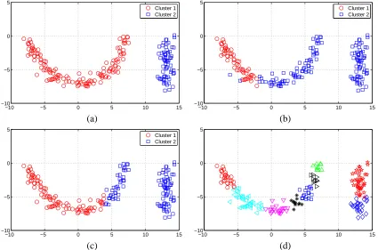
by mixture modeling are referred to Section 1.1. We will also show results of k-means clustering. The first data set, referred to as the noisy curve data set, contains a half circle and a straight line (or bar) imposed with noise, as shown in Figure 3(a). The circle centers at the origin and has radius 7. The line is a vertical segment between(13,−8) and(13,0). Roughly 2
3 of the 200 points are uniformly sampled from the half circle and 13 of them uniformly from the bar. Then, independent Gaussian noise with standard deviation 0.5 is added to both the horizontal and vertical directions of each point.
Consider clustering into two groups. The results of average linkage, mixture modeling, and k-means are shown in Figure 3(a), (b), (c). For this example, average linkage partitions the data perfectly into a noisy half circle and bar. Results of mixture modeling and k-means are close. In both cases, nearly one side of the half circle is grouped with the bar. In this example, the mixture model is initialized by the clustering obtained from k-means; and the covariance matrices of the two clusters are not restricted.
The second data set contains 200 samples generated as follows. The data are sampled from two clusters with prior probability 1/3 and 2/3 respectively. The first cluster follows a single Gaussian distribution with mean(6,0)and covariance matrix diag(1.52,1.52). The second cluster is generated by a mixture of two Gaussian components with prior probability 1/5 and 4/5, means(−3,0) and (0,0), and covariance matrices diag(32,32)and diag(1,1)respectively. The two clusters are shown in Figure 4(a). Again, we compare results of average linkage, mixture modeling, and k-means, shown in Figure 4(b), (c), (d). For mixture modeling, we use Mclust with three components and optimally selected covariance structures by BIC. Two of the three clusters generated by Mclust are combined to show the binary grouping. For this example, mixture modeling and k-means yield a partition close to the two original clusters, while average linkage gives highly skewed clusters, one of which contains a very small number of points on the outskirt of the mass of data.
−10 −5 0 5 10 15 −10
−5 0 5
Cluster 1 Cluster 2
−10 −5 0 5 10 15
−10 −5 0 5
Cluster 1 Cluster 2
(a) (b)
−10 −5 0 5 10 15
−10 −5 0 5
Cluster 1 Cluster 2
−10 −5 0 5 10 15
−10 −5 0 5
(c) (d)
Figure 3: Clustering results for the noisy curve data set. (a) The two original clusters. The two clusters obtained by average linkage clustering and HMAC are identical to the original ones. (b) Clustering by mixture modeling with two Gaussian components. (c) Clustering by k-means. (d) Clustering by HMAC at the first level of the hierarchy.
clusters closest to the original ones among all the methods. Comparing with mixture modeling, HMAC is more robust to the non-Gaussian cluster distributions.
−10 −5 0 5 10 −6
−4 −2 0 2 4 6 8
Cluster 1 Cluster 2
−10 −5 0 5 10
−6 −4 −2 0 2 4 6 8
Cluster 1 Cluster 2
(a) (b)
−10 −5 0 5 10
−6 −4 −2 0 2 4 6 8
Cluster 1 Cluster 2
−10 −5 0 5 10
−6 −4 −2 0 2 4 6 8
Cluster 1 Cluster 2
(c) (d)
−10 −5 0 5 10
−6 −4 −2 0 2 4 6 8
Cluster 1 Cluster 2
−10 −5 0 5 10
−6 −4 −2 0 2 4 6 8
(e) (f)
the latter are always local. While in HMAC, when the bandwidth increases, global characteristics of the data become highly influential on clustering results. Hence the clustering result tends to resemble that of mixture modeling (k-means) which enforces a certain kind of global optimality. In spite of this similarity, HMAC is more robust for clusters deviating from Gaussian distributions. In practice, it is usually preferable to ensure very close points are grouped together and in the mean time to generate clusters with global optimality. These two traits, however, are often at odds with each other, a phenomenon discussed in depth by Chipman and Tibshirani (2006).
Chipman and Tibshirani (2006) noted that bottom-up agglomerative clustering methods, such as average linkage, tend to generate good small clusters but suffer at extracting a few large clusters. The strengths and weaknesses of top-down clustering methods, such as k-means, are the opposite. A hybrid approach is proposed in that paper to combine the advantages of bottom-up and top-down clustering, which first seeks mutual clusters by bottom-up linkage clustering and then applies top-down clustering to the mutual clusters. HMAC also integrates the strengths of both types of clustering, in a way not as explicit as the hybrid method but more automatically.
To systematically study the performance of HMAC for high dimensional data and its stability over multiple implementations, we conduct the following experiment. We generate 55 random data sets each of dimension 50 and size 200. The first two dimensions of the data follow the distribution of the noisy curve data in the first example described. The other 48 dimensions are independent Gaussian noise all following the normal distribution with mean zero and standard deviation 0.5, same as the noise added to the half circle and line segment in the first two dimensions. As gold standard, we regard data generated by adding noise to the half circle as one cluster and those to the line segment as the other.
Clustering results are obtained for each of the 55 data sets using HMAC and Mclust respectively. For HMAC, the level of the dendrogram yielding two clusters is chosen to create the partition of the data. In another word, the basic version of HMAC is used without the separability based merging of clusters. For Mclust, we set the number of clusters to 2, but allow the algorithm to optimally select the structure of the covariance matrices using BIC. All the structural variations of the covariance matrices provided by Mclust are searched over. In Mclust, the mixture model is initialized using the suggested default option, that is, to initialize the partition of data by an agglomerative hierarchical clustering approach, an extension of linkage clustering based on Gaussian mixtures (Fraley and Raftery, 2006). This initialization may be of advantage especially to data in this study because as shown previously, linkage clustering generates perfect clustering for the noisy curve data set in the first example.
Denote each data set k, k=1,2, ...,55, by Ak={x(ik),i=1, ...,200}, where xi(k)= (xi(,k1),x(i,k2), ...,
x(i,k50))t. For each x(k)
i , we form a sequence of its lower dimensional vectors: x
(k,l)
i = (x
(k)
i,1,x (k)
i,2, ...,x
(k)
i,l )t,
l=2,3, ...,50. Let Ak,l ={xi(k,l),i=1, ...,200}. HMAC and Mclust are applied to every Ak,l,
l=2, ...,50, k=1, ...,55. Let the clustering error rate obtained by HMAC for Ak,l be r(kH,l) and
that by Mclust be r(kM,l). We summarize the clustering results in Figure 5.
5 10 15 20 25 30 35 40 45 50 20
30 40 50 60 70 80 90 100 110
Dimension
Percentage with non−perfect clustering (%)
HMAC Mclust
5 10 15 20 25 30 35 40 45 50 0
0.05 0.1 0.15 0.2 0.25 0.3
Dimension
Clustering error rate
HMAC, Average error rate HMAC, Median error rate Mclust, Average error rate Mclust, Median error rate
(a) (b)
Figure 5: Clustering results obtained by HMAC and Mclust for the 55 high dimensional noisy curve data sets. (a) The percentage of data sets that are not perfectly clustered with increasing dimensions. (b) The average and median of clustering error rates.
To examine clustering accuracy with respect to increasing dimensions, for each l=2, ...,50, the mean r(·,Hl), r(·,Ml ), and the median ˜r(·,Hl), ˜r(·,Ml )over the data sets are computed and shown in Figure 5(b).
For HMAC, the mean r(·,Hl) varies only slightly around 7.5% when the dimension increases, and
the median ˜r·,(Hl) stays at zero. The error rates obtained from Mclust, on the other hand, change
dramatically with the dimension. And for l =2 and l≥30, both r·,(Ml) and ˜r(·,Ml) are significantly
higher than r(·,Hl). Interestingly, the worst error rate from Mclust is achieved at l=2 with r(·,M2)>23% rather than at the high end of the range of dimensions. This seems to suggest that the extra noise dimensions help to mollify the effect of non-Gaussian shaped clusters. When l≥30, r(·,Ml)and ˜r·,(Ml ) increase steadily with the dimension and eventually reaches nearly 20%.
6.2 Real Data Sets
In this section, we apply HMAC to real data sets, compare our method of visualization described in Section 5 with PCA, and demonstrate the usage of the cluster merging algorithm described in Section 4.2.
6.2.1 GLASSDATA
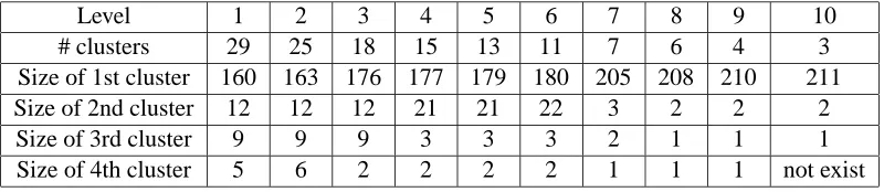
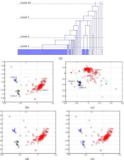
We first examine the aforementioned glass data set using the entire set of 214 samples and all the original 9 features. Applying HMAC, a dendrogram of 10 levels is obtained, as shown in Figure 6(a). The number of clusters at each level is listed in Table 2. The sizes of the largest 4 clusters at each level are also given in this table. The dendrogram and the table show that 3 clusters containing more than 5 points are formed at the first level. These 3 prominent clusters are retained or augmented up to level 3. At level 4, two of the 3 prominent clusters are merged, leaving 2 prominent clusters which are further merged at level 7. At this level, both the dendrogram and the table suggest the main clustering structure in the data is annihilated by the very large kernel bandwidth. However, the number of clusters generated at level 7 is 7 instead of 1. Except the largest cluster, the other 5 clusters each contain no more than 3 points and in total only 9. They may be considered more appropriately as “outliers” than clusters. At even higher levels, these tiny clusters are merged gradually into the main mass of data.
Level 1 2 3 4 5 6 7 8 9 10
# clusters 29 25 18 15 13 11 7 6 4 3
Size of 1st cluster 160 163 176 177 179 180 205 208 210 211 Size of 2nd cluster 12 12 12 21 21 22 3 2 2 2
Size of 3rd cluster 9 9 9 3 3 3 2 1 1 1
Size of 4th cluster 5 6 2 2 2 2 1 1 1 not exist
Table 2: The clustering results for the full glass data set.
The above discussion suggests that to obtain a given number of clusters, it is not always a good practice to choose a level in the hierarchy that yields the desired number of clusters. We may select a level at which major clusters are merged and outliers are mistaken as plausible clusters. One remedy is to apply the cluster merging algorithm to a larger number of clusters formed at a lower level. We will present results of this approach shortly.
To compare our visualization method with PCA, the clustering results at level 3 are shown in Figure 6(b) and (c) using the two projection methods respectively. Both projections are orthonormal. In our visualization method, the projection only attempts to approximate the discriminant functions between the 3 major clusters. It is obvious that the new visualization method shows the clustering structure better than PCA. The two projection directions derived by our method are used when presenting other clustering results for a clear correspondence between points in different plots.
Level 1 Level 3 Level 7 Level 10
(a)
−0.4 −0.2 0 0.2
−0.2 −0.15 −0.1 −0.05 0 0.05 0.1 0.15 0.2 0.25 0.3
Cluster 1
Cluster 2 Cluster 3
−0.4 −0.2 0 0.2 0.4 0.6 −0.5
−0.4 −0.3 −0.2 −0.1 0 0.1
Cluster 1
Cluster 2
Cluster 3
(b) (c)
−0.4 −0.2 0 0.2
−0.2 −0.15 −0.1 −0.05 0 0.05 0.1 0.15 0.2 0.25 0.3
−0.4 −0.2 0 0.2
−0.2 −0.15 −0.1 −0.05 0 0.05 0.1 0.15 0.2 0.25 0.3
(d) (e)