Ramp Loss Linear Programming Support Vector Machine
Xiaolin Huang [email protected]
Department of Electrical Engineering, ESAT-STADIUS, KU Leuven Kasteelpark Arenberg 10, Leuven, B-3001, Belgium
Lei Shi [email protected]
Department of Electrical Engineering, ESAT-STADIUS, KU Leuven
School of Mathematical Sciences, Fudan University, Shanghai, 200433, P.R. China
Johan A.K. Suykens [email protected]
Department of Electrical Engineering, ESAT-STADIUS, KU Leuven Kasteelpark Arenberg 10, Leuven, B-3001, Belgium
Editor:Mikhail Belkin
Abstract
The ramp loss is a robust but non-convex loss for classification. Compared with other non-convex losses, a local minimum of the ramp loss can be effectively found. The effec-tiveness of local search comes from the piecewise linearity of the ramp loss. Motivated by the fact that the `1-penalty is piecewise linear as well, the `1-penalty is applied for the ramp loss, resulting in a ramp loss linear programming support vector machine (ramp-LPSVM). The proposed ramp-LPSVM is a piecewise linear minimization problem and the related optimization techniques are applicable. Moreover, the`1-penalty can enhance the sparsity. In this paper, the corresponding misclassification error and convergence behavior are discussed. Generally, the ramp loss is a truncated hinge loss. Therefore ramp-LPSVM possesses some similar properties as hinge loss SVMs. A local minimization algorithm and a global search strategy are discussed. The good optimization capability of the proposed algorithms makes LPSVM perform well in numerical experiments: the result of ramp-LPSVM is more robust than that of hinge SVMs and is sparser than that of ramp-SVM, which consists of thek · kK-penalty and the ramp loss.
Keywords: support vector machine, ramp loss, `1-regularization, generalization error analysis, global optimization
1. Introduction
In a binary classification problem, the input space is a compact subset X ⊂ Rn and the output space Y ={−1,1} represents two classes. Classification algorithms produce binary classifiersC:X→Y induced by real-valued functionsf :X→RasC= sgn(f), where the
sign function is defined by sgn(f(x)) = 1 if f(x)≥0 and sgn(f(x)) =−1 otherwise. Since proposed by Cortes and Vapnik (1995), the support vector machine (SVM) has become a popular classification method, because of its good statistical property and generalization capability. SVM is usually based on a Mercer kernel K to produce non-linear classifiers. Such a kernel is a continuous, symmetric, and positive semi-definite function defined on
optimization problem
min f∈HK,b∈R
µ
2kfk
2
K+
1
m m
X
i=1
L(1−yi(f(xi) +b)), (1)
whereHK is the Reproducing Kernel Hilbert Space (RKHS) induced by the Mercer kernel
K with the normk · kK(Aronszajn, 1950) andµ >0 is a trade-off parameter. The constant
term bis called offset, which leads to much flexibility. The corresponding binary classifier is evaluated based on the optima of (1) by its sign function. Traditionally, the hinge loss
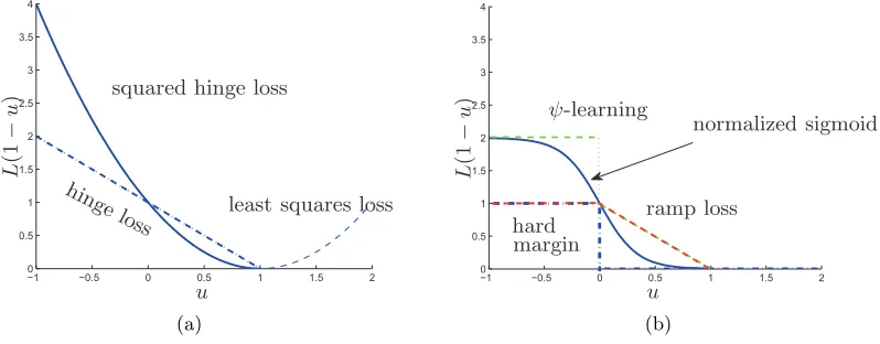
Lhinge(u) = max{u,0}is used. Besides, the squared hinge loss (Vapnik, 1998) and the least squares loss (Suykens and Vandewalle, 1999; Suykens et al., 2002) also have been widely applied. In classification and the related methodologies, robustness to outliers is always an important issue. The influence function (see, e.g., Steinwart and Christmann, 2008; De Brabanter et al., 2009) related to the hinge loss is bounded, which means that the effect of outliers on the result of minimizing the hinge loss is bounded. Though the effect is bounded, it can be significantly large since the penalty given to the outliers by the hinge loss is quite huge. In fact, any convex loss is unbounded. To remove the effect of outliers, researchers turn to some non-convex losses, such as the hard-margin loss, the normalized sigmoid loss (Mason et al., 2000), theψ-learning loss (Shen et al., 2003), and the ramp loss (Collobert et al., 2006a,b). The ramp loss is defined as follows,
Lramp(u) =
Lhinge(u), u≤1,
1, u >1,
which is also called a truncated hinge loss in Wu and Liu (2007). The plots of the mentioned losses are illustrated in Figure 1, showing the robustness of these non-convex losses.
−1 −0.5 0 0.5 1 1.5 2
0 0.5 1 1.5 2 2.5 3 3.5 4
u
L
(1
−
u
)
hing e loss
squared hinge loss
least squares loss
(a)
−1 −0.5 0 0.5 1 1.5 2
0 0.5 1 1.5 2 2.5 3 3.5 4
u
L
(1
−
u
)
ramp loss
normalized sigmoid
hard margin
ψ-learning
(b)
Among the mentioned robust but non-convex losses, the ramp loss is an attractive one. Using the ramp loss in (1), one obtains a ramp loss support vector machine (ramp-SVM). Because the ramp loss can be easily written as a difference of convex functions (DC), algorithms based on DC programming are applicable for ramp-SVM. The discussion about DC programming can be found in An et al. (1996), Horst and Thoai (1999), and An and Tao (2005). To apply DC programming in the ramp loss, we first observe the identity
Lramp(u) = min{max{u,0},1}= max{u,0} −max{u−1,0}. (2) Therefore, SVM (1) with L = Lramp can be decomposed into the convex part µ2kfk2
K+
1 m
Pm
i=1max{1−yi(f(xi) +b),0} and the concave part −m1
Pm
i=1max{−yi(f(xi) +b),0}. Hence DC programming can be used for finding a local minimizer of this problem, which has been applied by Collobert et al. (2006a), Wu and Liu (2007). DC programming for ramp-SVM is also referred to as a concave-convex procedure by Yuille and Rangarajan (2003). Besides the continuous optimization methods, ramp-SVM has been formulated as a mixed integer optimization problem by Brooks (2011) as below,
min f∈HK,b∈R,ω
µ 2kfk
2
K+ m1
Pm
i=1(ei+ωi)
s.t. ωi ∈ {0,1},
0≤ei≤1, i= 1,· · ·, m,
yi(f(xi) +b)≥1−ei, ifωi = 0.
(3)
The optimization problem (3) should be solved over all possible binary vectorsω= [ω1, . . . , ωm]T ∈ {0,1}m. Once the binary vectorωis given, this problem can be solved by quadratic programming. Consequently, when the size of the problem grows, the computation time explodes.
It is worth noting the case of taking L=Lhingein (1). It corresponds to the well-known
C-SVM. One can solve C-SVM by its dual form, then the output function is represented as
Pm
i=1νi∗yiK(x, xi) +b∗, where [ν1∗,· · ·, νm∗]T is the optimal solution of min
νi∈R
1 2
Pm
i,j=1νiνjyiyjK(xi, xj)−Pmi=1νi s.t. Pm
i=1νiyi = 0,
0≤νi ≤ µm1 , i= 1,· · ·, m.
The optimal offset b∗ can be computed from the Karush-Kuhn-Tucker (KKT) conditions after {νi∗}m
i=1 is found (see, e.g., Suykens et al., 2002). From the dual form of C-SVM, we
find that though we search the functionf in a rather large spaceHK, the optimal solution
actually belongs to a finite-dimensional subspace given byH+
K,z with
H+K,z=nXm
i=1αiyiK(x, xi),∀α= [α1, . . . , αm]
T 0o.
Here the notation0 means all the elements of the vector being non-negative.
To enhance the sparsity in the output function, the linear programming support vector machine (LPSVM) directly minimizes the data fitting term m1 Pm
i=1Lhinge(1−yi(f(xi) +b)) with a `1-penalty term (see Vapnik, 1998; Smola et al., 1999). Given f ∈ H+K,z, the `1 -penalty is defined as
Ω(f) = m
X
i=1
αi, forf = m
X
i=1
which is the`1-penalty of the combinatorial coefficients of f. Then LPSVM can be
formu-lated as follows,
min f∈H+K,b∈R
µΩ(f) + 1
m m
X
i=1
Lhinge(1−yi(f(xi) +b)). (5)
LPSVM is also related to 1-norm SVM proposed by Zhu et al. (2004), which searches a linear combination of basis functions and does not consider the non-negative constraint. The properties of LPSVM have been demonstrated in the literature (e.g., Bradley and Mangasarian, 2000; Kecman and Hadzic, 2000). Generalization error analysis for LPSVM can be found in Wu and Zhou (2005).
For problem (1), one can choose different penalty terms and different loss functions. For example, using kfkK together with the hinge loss, we obtain C-SVM. The property of
C-SVM can be observed from the properties of kfkK and the hinge loss: since kfkK is a
quadratic function and the hinge loss is piecewise linear (pwl), the objective function of C-SVM is piecewise quadratic (pwq) and can be solved by constrained quadratic programming. For LPSVM, which consists of the `1-penalty and the hinge loss, the objective function is convex piecewise linear and hence can be minimized by linear programming. In Table 1, we summarize the properties of several penalties and losses.
squared least ψ- normalized
kfkK Ω(f) hinge hinge squares learning sigmoid ramp
function type quadratic pwl pwl pwq quadratic discontinuous log pwl
convexity √ √ √ √ √ × × ×
continuity √ √ √ √ √ × √ √
smoothness √ × × √ √ × √ ×
sparsity × √ √ √ × √ × √
bounded
influence fun. — — √ × × √ √ √
bounded
penalty value — — × × × √ √ √
∗
“pwl” stands for piecewise linear; “pwq” stands for piecewise quadratic.
Table 1: Properties of Different Penalties and Losses
The ramp loss gives a constant penalty for any large outlier and it is obviously robust. From Table 1, we observe that both Ω(f) and the ramp loss are continuous piecewise linear. It follows that if we choose Ω(f) and the ramp loss, the objective function of (1) is continuous piecewise linear and can be minimized by linear programming. Besides, minimizing Ω(f) enhances the sparsity. Motivated by this observation, in this paper we study the binary classifiers generated by minimizing the ramp loss and the`1-penalty, which is called a ramp
loss linear programming support vector machine (ramp-LPSVM). The ramp-LPSVM has the following formulation,
(fz,µ∗ , b∗z,µ) = argmin f∈H+K,z,b∈R
µΩ(f) + 1
m m
X
i=1
where Ω(·) is the`1-penalty defined by (4). And the induced classifier is given by sgn(fz,µ∗ + b∗z,µ). We call (6) ramp-LPSVM, which implies that the algorithm proposed later involves linear programming problems. Similarly to ramp-SVM, the proposed ramp-LPSVM enjoys robustness. Moreover, it can give a sparser solution. In addition to enhancing the sparsity, replacing thek · kK-penalty in ramp-SVM by the`1-penalty is mainly motivated by the fact
that both the ramp loss and the `1-penalty are piecewise linear, which helps developing
more efficient algorithms.
Resulting from the identity (2), the problem related to ramp-LPSVM leads to a polyhe-dral concave problem, which minimizes a concave function on one polyhedron. A polyhepolyhe-dral concave problem is easier to handle than a regular non-convex problem and some efficient methods were reviewed by Horst and Hoang (1996). Moreover, ramp-LPSVM (6) has a piecewise linear objective function. For such kind of problems, a hill detouring technique proposed by Huang et al. (2012a) has shown good global search capability. As the name sug-gests, the hill detouring method searches on the level set to escape from a local optimum. One contribution of this paper is that we establish algorithms for solving ramp-LPSVM (6), including DC programming for local minimization and hill detouring for global search. Additionally, we investigate the asymptotic performance of ramp-LPSVM under the frame-work of statistical learning theory. Our analysis implies that ramp-LPSVM has a similar misclassification error bound and similar convergence behavior as C-SVM. Moreover, one can expect that the output binary classifier of algorithm (6) is robust, due to the ramp loss, and has a sparse representation, due to the `1-penalty.
The remainder of the paper is organized as follows: some statistical properties for the proposed ramp-LPSVM are discussed in Section 2. In Section 3, we establish problem-solving algorithms including DC programming for local minimization, and hill detouring for escaping from local optima. The proposed algorithms are tested then on numerical experiments in Section 4. Section 5 ends the paper with concluding remarks.
2. Theoretical Properties
In this section, we establish the theoretical analysis for ramp-LPSVM under the framework of statistical learning theory. In the following, we first show that the ramp loss is classifica-tion calibrated; see Proposiclassifica-tion 1. In other works, we prove that minimizing the ramp loss results in the Bayes classifier. After that, an inequality is presented in Theorem 2 to bound the difference between the risk of the Bayes classifier and that of the classifier induced from minimizing the ramp loss. Finally, we obtain the convergence behavior of ramp-LPSVM, which is given in Theorem 5. To prove Theorem 5, error decomposition theorems for ramp-SVM and ramp-LPramp-SVM are discussed. The analysis on the ramp loss is closely related to the properties of the hinge loss, because the ramp loss can be regarded as a truncated hinge loss. In our analysis, the global minimizer of the ramp loss plays an important role, which motivates us to establish a global search strategy in the next section.
To this end, we assume that the sample z ={xi, yi}mi=1 is independently drawn from a
probability measureρonX×Y. The misclassification error for a binary classifierC:X→Y
is defined as the probability of the event C(x)6=y:
R(C) =
Z
X×Y
Iy6=C(x)dρ=
Z
X
where I is the indicator function, ρX is the marginal distribution of ρ on X, and ρ(y|x) is the conditional distribution of ρ at given x. It should be pointed out that ρ(y|x) is a binary distribution, which is given by Prob(y = 1|x) and Prob(y = −1|x). The classifier that minimizes the misclassification error is the Bayes rule fc, which is defined as,
fc= arg min
C:X→YR(C).
The Bayes rule can be evaluated as
fc(x) =
1, if Prob(y= 1|x)≥Prob(y=−1|x), −1, if Prob(y= 1|x)<Prob(y=−1|x).
The performance of a binary classifier induced by a real-valued function f is measured by the excess misclassification errorR(sgn(f))− R(fc).Let fz,µ =fz,µ∗ +b∗z,µ with (fz,µ∗ , b∗z,µ) being the global minimizer of ramp-LPSVM (6). The purpose of the theoretical analysis is to estimateR(sgn(fz,µ))− R(fc) as the sample sizem tends to infinity. Convergence rates will be derived under the choice of the parameter µand conditions on the distributionρ.
As an important ingredient in classification algorithms, the loss function L is used to model the target function of interest. Concretely, the target function denoted as fL,ρ minimizes the expected L-risk
RL,ρ(f) =
Z
X×Y
L(1−yf(x))dρ
over all possible functions f :X →Rand can be defined pointwisely as below,
fL,ρ(x) = arg min t∈R Z
Y
L(1−yt)dρ(y|x), ∀x∈X.
The basic idea on designing algorithms is to replace the unknown true risk RL,ρ by the empiricalL-risk
RL,z(f) = 1
m m
X
i=1
L(1−yif(xi)), (7)
and to minimize this empirical risk (or its penalized version) over a suitable function class. When the hard margin loss, which counts the number of misclassification,
Lmis(u) =
0, u≥0,
1, u <0,
is used, one can check that for any binary classifier C : X → Y, there holds R(C) =
RLmis,ρ(C).Therefore, the excess misclassification error can be written as
RLmis,ρ(sgn(f))− RLmis,ρ(fc).
However, the empirical algorithms based on Lmis will lead to NP-hard optimization
risk associated with the used surrogate loss. Among these losses, the hinge loss plays an important role, since one hasfLhinge,ρ=fc.
Now we investigate the ramp loss. For a givenx∈X, a simple calculation shows that
Z
Y
Lramp(1−yt)dρ(y|x)
= Lramp(1−t)Prob(y= 1|x) +Lramp(1 +t)Prob(y=−1|x)
=
Prob(y= 1|x), t≤ −1,
Prob(y= 1|x) + (1 +t)Prob(y=−1|x), −1< t≤0,
(1−t)Prob(y= 1|x) + Prob(y=−1|x), 0≤t <1,
Prob(y=−1|x), t≥1.
Obviously, when Prob(y = 1|x) >Prob(y = −1|x), the minimal value is Prob(y =−1|x), which is achieved by t = 1. When Prob(y = 1|x) < P(y = −1|x), the minimal value is Prob(y = 1|x), which is achieved by t=−1. Therefore, the corresponding target function
fLramp,ρ that minimizes the expectedLramp-risk is the Bayes rule. The discussion above can be concluded in the following proposition.
Proposition 1 For any measurable function f :X →R, there holds
RLramp,ρ(f)≥ RLramp,ρ(fc).
That is, the Bayes rule fc is a minimizer of the expectedLramp-risk.
Next, for a real-valued function f :X → R, we consider bounding the excess
misclas-sification error by the generalization error RLramp,ρ(f)− RLramp,ρ(fLramp,ρ). Such kind of bound plays an essential role in error analysis of classification algorithms. When the loss function is convex and satisfies some regularity conditions, the corresponding bound is the so-called self-calibration inequality and has been established by Bartlett et al. (2006) and Steinwart (2007). For example, a typical result presented in Cucker and Zhou (2007) claims that, if a general loss function satisfies the following conditions:
• L(1−u) is convex with respect tou;
• L(1−u) is differentiable atu= 0 and dL(1du−u)|u=0 <0;
• min{u:L(1−u) = 0}= 1;
• d2Ldu(12−u)|u=1 >0,
then there exists a constantcL>0 such that for any measurable function f :X →R,
RLmis,ρ(sgn(f))− RLmis,ρ(fc)≤cL
q
This inequality holds for many loss functions, such as the hinge loss, the squared hinge loss, and the least squares loss. For the hinge lossLhinge, Zhang (2004) gave a tighter bound by the following inequality,
RLmis,ρ(sgn(f))− RLmis,ρ(fc)≤ RLhinge,ρ(f)− RLhinge,ρ(fLhinge,ρ).
The improvement is mainly due to the property that RLhinge,ρ(fLhinge,ρ) =RLhinge,ρ(fc). For the ramp lossLramp, we cannot directly use the conclusion given by (8), since the loss
is not convex. However, asLrampcan be considered as a truncated hinge loss and maintains
the same property due to Proposition 1, one thus can establish a similar inequality for the ramp loss.
Theorem 2 For any probability measure ρ and any measurable function f :X →R,
RLmis,ρ(sgn(f))− RLmis,ρ(fc)≤ RLramp,ρ(f)− RLramp,ρ(fLramp,ρ). (9)
Proof By Proposition 1, we have RLramp,ρ(fLramp,ρ) = RLramp,ρ(fc). Since y and fc(x) belong to{−1,1}, 1−yfc(x) takes value of 0 or 2. We hence haveRLmis,ρ(fc) =RLramp,ρ(fc), which comes from the fact that
Lmis(0) =Lramp(0) and Lmis(2) =Lramp(2).
Thus, to prove (9), we need to show that
RLmis,ρ(sgn(f))≤ RLramp,ρ(f), (10)
which is equivalent to
Z
X×Y Lmis
1−ysgn(f(x))
−Lramp
1−yf(x)
dρ≤0.
For any y and f(x), if yf(x) ≤ 0, then ysgn(f(x)) ≤ 0, which follows that Lmis(1− ysgn(f(x))) = Lramp(1−yf(x)) = 1. If yf(x) > 0, then we have ysgn(f(x)) = 1 and Lmis(1−ysgn(f(x))) = 0. Since Lramp(1−yf(x)) is always nonnegative, we haveLmis(1− ysgn(f(x)))−Lramp(1−yf(x))≤0 for this case.
Summarizing the above discussion, we prove (10) and then Theorem 2.
From Theorem 2, in order to estimateRLmis,ρ(sgn(fz,µ))− RLmis,ρ(fc), we turn to bound RLramp,ρ(fz,µ)− RLramp,ρ(fc). We thus need an error decomposition for the latter. This decomposition process is well-developed in the literature for RKHS-based regularization schemes (see, e.g., Cucker and Zhou, 2007; Steinwart and Christmann, 2008). To explain the details, we take ramp-SVM below as an example. For z = {xi, yi}mi=1 and λ >0, let
˜
fz,λ= ˜fz,λ∗ + ˜b∗z,λ, where
( ˜fz,λ∗ ,˜b∗z,λ) = argmin f∈HK,b∈R
λ
2kfk
2
K+
1
m m
X
i=1
Then the following decomposition holds true:
RLramp,ρ( ˜fz,λ)− RLramp,ρ(fc) ≤
n
RLramp,ρ( ˜fz,λ)− RLramp,z( ˜fz,λ)
o
+
RLramp,z(fλ)− RLramp,ρ(fλ) +A(λ),
where RLramp,z(f) is the empirical Lramp-risk given by (7). The functionfλ depends onλ and is defined by the data-free limit of (11), that is fλ =fλ∗+b∗λ with
(fλ∗, b∗λ) = argmin f∈HK,b∈R
λ
2kfk
2
K+Rramp,ρ(f+b). (12)
The term A(λ) measures the approximation power of the system (K, ρ) and is defined by
A(λ) = inf f∈HK,b∈R
λ
2kfk
2
K+Rramp,ρ(f +b)− Rramp,ρ(fc), ∀λ >0. (13) It is easy to establish such kind of decomposition if one notices the fact that both ˜fz,λ and fλ lie in the same function space. However, it is not the case for ramp-LPSVM. The data-dependent nature ofH+K,zleads to an essential difficulty in the error analysis. Motivated by Wu and Zhou (2005), we shall establish the error decomposition for ramp-LPSVM (6) with the aid of ˜fz,λ. To this end, we first show some properties of ˜fz,λ, which play an important role in our analysis.
Proposition 3 For any λ > 0, ( ˜fz,λ∗ ,˜b∗z,λ) is given by (11) and f˜z,λ = ˜fz,λ∗ + ˜b∗z,λ. Then ˜
fz,λ∗ ∈ H+K,z and
Ω( ˜fz,λ∗ )≤λ−1RLramp,z( ˜fz,λ) +kf˜z,λ∗ k2K. (14)
Proof Following the idea of Brooks (2011), one can formulate the minimization problem (11) as a mixed integer optimization problem, which is given by (3) with µ =λ. We first show that if the binary vector ω∗ = [ω1∗,· · ·, ωm∗]T ∈ {0,1}m is optimal for the optimization problem (3), then the global minimizer of (11) can be obtained by solving the following minimization problem
min f∈HK,ei,b∈R
λ
2kfk2K+m1
Pm
i=1ei
s.t. ei ≥0, i= 1,· · ·, m,
yi(f(xi) +b)≥1−ei, ifωi∗= 0.
(15)
In fact, when the optimal ω∗ is given, the global minimizer of (11) can be solved by the optimization problem (3), which is reduced to
min f∈HK,ei,b∈R
λ
2kfk2K+m1
Pm
i=1ei s.t. 0≤ei ≤1, i= 1,· · ·, m,
yi(f(xi) +b)≥1−ei, ifωi∗= 0.
(16)
withe∗1= [e∗11,· · ·, e∗m1]T. As the constraints in problem (16) is a subset of that in problem (15), we thus have
λ
2k ˜
fz,λ1 k2
K+ 1 m m X i=1
e∗i1 ≤ λ
2k ˜
fz,λ∗ k2
K+ 1 m m X i=1 e∗i.
To prove our claim, we just need to verify that 0≤e∗i1 ≤1 for i= 1,· · ·, m. For ωi∗ = 1, it is easy to see that e∗i1 = 0. Next we prove the conclusion for the case ωi∗ = 0. Define an index set as I := {i∈ {1,· · ·, m} :ωi∗ = 0 and e∗i1 >1}. If I is an non-empty set, we further define a binary vector ω0 withω0i = 1 for i ∈I and ωi0 =ωi∗ otherwise. As ωi = 1 implies the corresponding optimal ei should equal 0, we then define e0i as e0i = 0 if ωi0 = 1 and e0i =e∗i1 otherwise. One can check that
λ
2kf˜
1 z,λk2K+
1
m m
X
i=1
(e0i+ωi0)< λ
2kf˜
1 z,λk2K+
1
m m
X
i=1
(e∗i1+ωi∗)≤ λ
2kf˜
∗
z,λk2K+
1
m m
X
i=1
(e∗i +ωi∗).
We thus derive a contradiction to the assumption that ( ˜fz,λ∗ ,˜b∗z,λ, e∗, ω∗) is a global optimal solution for problem (3) and the conclusion follows.
Now we can prove our desired result based on the optimization problem (15). Let
I0 = {i : ω∗i = 0} and I1 = {i : ωi∗ = 1}. Since the triple ( ˜fz,λ∗ ,˜b∗z,λ, e∗) is the optimal solution of problem (15), from the KKT condition, there exist constants{α˜∗i}i∈I0, such that
˜
fz,λ∗ (x) =X i∈I0
˜
αi∗yiK(xi, x) with 0≤α˜∗i ≤ 1
λm,
X
i∈I0 ˜
α∗iyi= 0,
1−yi( ˜fz,λ∗ (xi) + ˜b∗z,λ)≤0, ifi∈I0 and ˜α∗i = 0,
0≤e∗i = 1−yi( ˜fz,λ∗ (xi) + ˜b∗z,λ)≤1, ifi∈I0 and ˜α∗i 6= 0.
We also have e∗i = 0, ifi ∈ I1. Moreover, by the same argument used in the proof about
the equivalence of problems (15) and (16), one can find that when i ∈ I1, we must have 1−yi( ˜fz,λ∗ (xi) + ˜b∗z,λ)>1 or 1−yi( ˜fz,λ∗ (xi) + ˜b∗z,λ)<0 due to the optimality of ω∗.
From the expression of ˜fz,λ∗ , we can write ˜fz,λ∗ as Pm
i=1α
∗
iyiK(xi, x) with α∗i = ˜α∗i if i∈I0 and α∗i = 0 otherwise. Then ˜fz,λ∗ ∈ HK+,z. Furthermore, the relation P
i∈I0α˜
∗
iyi = 0 implies P
i∈I0α˜
∗
iyi˜b∗z,λ= 0. Then we have
Ω( ˜fz,λ∗ ) =X i∈I0
˜
α∗i =X i∈I0
˜
αi∗(1−yi( ˜fz,λ∗ (xi) + ˜b∗z,λ)) +
X
i∈I0 ˜
α∗iyif˜z,λ∗ (xi).
Note that ˜fz,λ∗ (x) =P
i∈I0α˜
∗
iyiK(xi, x). By the definition ofk · kK-norm, it follows that
X
i∈I0 ˜
α∗iyif˜z,λ∗ (xi) =
X
i,j∈I0 ˜
Additionally, based on our analysis, we also have
X
i∈I0 ˜
αi∗(1−yi( ˜fz,λ∗ (xi) + ˜b∗z,λ)) =
X
i∈I0 ˜
α∗iLramp(yi( ˜fz,λ∗ (xi) + ˜b∗z,λ))≤λ
−1R
Lramp,z( ˜fz,λ).
Hence the bound for Ω( ˜fz,λ∗ ) follows.
Now we are in the position to make an error decomposition for ramp-LPSVM.
Theorem 4 For0< µ ≤λ≤1, let η= µλ. Recall that fz,µ =fz,µ∗ +b∗z,µ where (fz,µ∗ , b∗z,µ)
is a global minimizer of ramp-LPSVM (6) and fλ = fλ∗+b
∗
λ with (f
∗
λ, b
∗
λ) given by (12).
Define the sample error S(m, µ, λ) as below,
S(m, µ, λ) =RLramp,ρ(fz,µ)− RLramp,z(fz,µ) + (1 +η)
RLramp,z(fλ)− RLramp,ρ(fλ) .
Then there holds
RLramp,ρ(fz,µ)− Rramp,ρ(fc) +µΩ(fz,µ∗ )≤ηRLramp,ρ(fc) +S(m, µ, λ) + 2A(λ), (17)
where A(λ) is the approximation error given by (13).
Proof Recall that for any λ >0, ˜fz,λ= ˜fz,λ∗ + ˜b
∗
z,λ where ( ˜f
∗
z,λ,˜b
∗
z,λ) is given by (11). Due to the definition of fz,µ and the fact ˜fz,λ∗ ∈ H+K,z, we have
RLramp,z(fz,µ) +µΩ(fz,µ∗ )≤ RLramp,z( ˜fz,λ) +µΩ( ˜fz,λ∗ ).
Proposition 3 gives
Ω( ˜fz,λ∗ )≤λ−1RLramp,z( ˜fz,λ) +kf˜z,λ∗ k2K.
Hence,
RLramp,z(fz,µ) +µΩ(fz,µ∗ )≤
1 +µ
λ
RLramp,z( ˜fz,λ) +µkf˜z,λ∗ k2K.
This enables us to boundRLramp,ρ(fz,µ) +µΩ(fz,µ∗ ) as
RLramp,ρ(fz,µ) +µΩ(fz,µ∗ ) ≤
RLramp,ρ(fz,µ)− RLramp,z(fz,µ)
+
1 +µ
λ
RLramp,z( ˜fz,λ) +µkf˜z,λ∗ k2K.
Next we use the definitions of ˜fz,λandfλ to analyze the last two terms of the above bound:
1 +µ
λ
RLramp,z( ˜fz,λ) +µkf˜
∗
z,λk2K
≤1 +µ
λ RLramp,z( ˜fz,λ) +λkf˜
∗
z,λk2K
≤1 +µ
λ
RLramp,z(fλ) +λkfλ∗k2K
=
1 +µ
λ
RLramp,z(fλ)− RLramp,ρ(fλ) +RLramp,ρ(fλ) +λkfλ∗k2K
Combining the above estimates, we find thatRLramp,ρ(fz,µ)− Rramp,ρ(fc) +µΩ(fz,µ∗ ) can be bounded by
RLramp,ρ(fz,µ)− RLramp,z(fz,µ) +
1 +µ
λ
RLramp,z(fλ)− RLramp,ρ(fλ)
+1 +µ
λ
RLramp,ρ(fλ)− RLramp,ρ(fc) +λkfλ∗k2K +
µ
λRLramp,ρ(fc).
Recalling the definition offλ, one hasA(λ) =RLramp,ρ(fλ)− RLramp,ρ(fc) +λkfλ∗k2K. Hence
the desired result follows.
With the help of Theorem 4, the generalization error is estimated by boundingS(m, µ, λ) and A(λ) respectively. As the ramp loss is Lipschitz continuous, one can show that
Rramp,ρ(f)− Rramp,ρ(fc)≤ kf−fckL1
ρX.
Hence the approximation error A(λ) can be estimated by the approximation in a weighted
L1 space with the norm kfkL1
ρX =
R
X|f(x)|dρX, as done in Smale and Zhou (2003). The following assumption is standard in the literature of learning theory (see, e.g., Cucker and Zhou, 2007; Steinwart and Christmann, 2008).
Assumption 1 For any 0< β≤1 and cβ >0, the approximation error satisfies
A(λ)≤cβλβ, ∀λ >0. (18)
We also expect that the sample error S(m, λ, µ) will tend to zero at a certain rate as the sample size tends to infinity. The asymptotical behaviors of S(m, λ, µ) can be illustrated by the convergence of the empirical mean m1 Pm
i=1ςi to its expectation Eςi, where {ςi} m i=1
are independent random variables defined as
ςi =Lramp(yif(xi)). (19) At the end of this section, we present our main theorem to illustrate the convergence behavior of ramp-LPSVM (6).
Theorem 5 Suppose that Assumption 1 holds with 0 < β ≤ 1. Take µ = m−4ββ+1+2 and fz,µ=fz,µ∗ +b∗z,µ with(fz,µ∗ , b∗z,µ) being the global minimizer of ramp-LPSVM (6). Then for
any0< δ <1, with probability at least 1−δ, there holds
RLmis,ρ(sgn(fz,µ))− RLmis,ρ(fc)≤˜c
log4
δ
1/2
m−4ββ+2, (20)
where c˜is a constant independent δ or m.
for ramp-LPSVM (6), so the derived convergence rates of the latter are essentially no worse than those of ramp-SVM. Actually, also from our discussion in this section, ramp-SVM and C-SVM should have almost the same error bounds. One thus can expect that ramp-LPSVM enjoys similar asymptotic behaviors as C-SVM. It also should be pointed that, throughout our analysis, the global optimality plays an important role. Therefore, to guarantee the performance of ramp-LPSVM, a global search strategy is necessary.
3. Problem-solving Algorithms
In the previous section, we discussed theoretical properties for ramp-LPSVM. Its robustness and sparsity can be expected, if a good solution of ramp-LPSVM (6) can be obtained. However, (6) is non-convex. Therefore, in this paper, we propose a downhill method for local minimization and a heuristic for escaping a local minimum. Difference of convex function (DC) programming proposed by An et al. (1996) and An and Tao (2005) has been applied for ramp loss minimization problems (see Wu and Liu, 2007; Wang et al., 2010). By Yuille and Rangarajan (2003), Collobert et al. (2006b), Zhao and Sun (2008), this type of methods is also called a concave-convex procedure. For the proposed ramp-LPSVM, the DC technique is applicable as well.
Let α = [α1,· · ·, αm]T ∈ Rm. Based on the identity (2), ramp-LPSVM (6) can be
written as follows,
min α0,b µ
m
X
i=1 αi+
1
m m
X
i=1
max
1−yi
m
X
j=1
αjyjK(xi, xj) +b
,0
−1 m
m
X
i=1
max
−yi
m
X
j=1
αjyjK(xi, xj) +b
,0
. (21)
We let ζ = [αT, b]T stand for the optimization variable and D(ζ) for the feasible set of (21). Denote the convex part (the first line of ) as g(ζ), and the concave part (the second line of (21)) as h(ζ). After that, (21) can be written as minζ∈D(ζ)g(ζ)−h(ζ). Then DC
programming developed by Horst and Thoai (1999) and An and Tao (2005) is applicable. We give the following algorithm for local minimization for ramp-LPSVM.
Algorithm 1:DC programming for ramp-LPSVM from ˆα,ˆb •Setδ >0,k:= 0 andζ0 := [ ˆαT,ˆb]T;
repeat
•Select ηk∈∂h(ζk); •ζk+1 := arg min
ζ∈D(ζ)g(ζ)
− h(ζk) + (ζ−ζk)Tηk
;
•Set k:=k+ 1;
untilkζk−ζk−1k< δ;
•Algorithm ends and returns ζk.
The non-differentiability ofh(ζ) comes from max{u,0}, of which the sub-gradient at u= 0 is in the interval [0,1]:
∂max{u,0} ∂u
u=0 ∈[0,1].
In our algorithm, we choose 0.5 as the value of the above sub-gradient and thenηk∈∂h(ζk) is uniquely defined. The local optimality condition for DC problems has been investi-gated by An and Tao (2005) and references therein. For a differentiable function, one can use the gradient information to check whether the solution is locally optimal. However, ramp-LPSVM is non-smooth and a sub-gradient technique should be considered. The local minimizer of a non-smooth objective function should meet the local optimality condition for all vectors in its sub-gradient set. In Algorithm 1, we only consider one value of the sub-gradient, thus, the result of the above process is not necessarily a local minimum. The rigorous local optimality condition and the related algorithm can be found in Huang et al. (2012b). However, because of the effectiveness of DC programming, we suggest Algorithm 1 for ramp-LPSVM in this paper.
As a local search algorithm, DC programming can effectively decrease the objective value of (21). The main difficulty of solving (21) is that it is non-convex and hence we may be trapped in a local optimum. To escape from a local optimum, we introduce slack variable
c= [c1,· · ·, cm]T and transform (21) into the following concave minimization problem,
min α,b,c µ
m
X
i=1 αi+
1
m m
X
i=1 ci−
1
m m
X
i=1
max
−yi
m
X
j=1
αjyjK(xi, xj) +b
,0
s.t. ci ≥1−yi
Xm
j=1αjyjK(xi, xj) +b
, i= 1,2, . . . , m, (22)
ci ≥0, i= 1,2, . . . , m, αi ≥0, i= 1,2, . . . , m.
This is a concave minimization problem constrained in a polyhedron, which is called a polyhedral concave problem by Horst and Hoang (1996). Generally, among non-convex problems, a polyhedral concave problem is relatively easy to deal with. Various techniques, such as γ-extension, vertex enumeration, partition algorithm, concavity cutting, have been discussed insightfully in Horst and Hoang (1996) and successfully applied (see, e.g., Porem-bski, 2004; Mangasarian, 2007; Shu and Karimi, 2009). Moreover, the objective function of (22) is piecewise linear, which makes the hill detouring method proposed by Huang et al. (2012a) applicable. In the following, we first introduce the basic idea of the hill detouring method and then establish a global search algorithm for ramp-LPSVM.
For notational convenience, we use ξ= [αT, b, cT]T to denote the optimization variable of (22). The objective function is continuous piecewise linear and is denoted as p(ξ). The feasible set, which is a polyhedron, can be written as Aξ ≤ q. Then (22) is compactly represented as the following polyhedral concave problem, of which the objective function is piecewise linear:
minξ p(ξ), s.t. Aξ≤q. (23)
vertex of the feasible set; ii) any level set{ξ :p(ξ) =u},∀uis the boundary of a polyhedron. The first property can be derived from the concavity of the objective function. The second property comes from the piecewise linearity ofp(ξ). These properties imply a new method searching on the level set to find another feasible solution ˆξ with the same objective value
p( ˆξ) = ˜p. If such ˆξ is found, we escape from ˜ξ and a downhill method can be used to find a new local optimum. Otherwise, if such ˆξ does not exist, one can conclude that ˜ξ is the optimal solution. Searching on the level set of p(ξ) = ˜p will not decrease neither increase the objective value and it is hence called hill detouring. In practice, in order to avoid to find
˜
ξ again, we search on{p(ξ) = ˜p−ε}with a small positiveεfor computational convenience. If {p(ξ) = ˜p−ε} =∅, we know that ˜ξ is ε-optimal. The performance of hill detouring is not sensitive to the εvalue, when εis small (but large enough to distinguish ˜p−and ˜p). In this paper, we set ε= 10−6.
Hill detouring, which is to solve the feasibility problem
find ξ, s.t. p(ξ) = ˜p−ε, Aξ ≤q, (24)
is a natural idea for global optimization but it is hard to implement for a regular concave minimization functions. The main difficulty is the nonlinear equationp(ξ) = ˜p−ε. In ramp-LPSVM, the objective function of (22) is continuous and piecewise linear, thus,p(ξ) = ˜p−ε
can be transformed into (finite) linear equations. That means (24) can be written as a series of LP feasibility problems, which makes line search on {ξ:p(ξ) = ˜p−ε} possible.
To investigate the property of (23) and the corresponding hill detouring technique, we consider a 2-dimensional problem. In this intuitive example, the objective function is
p(ξ) =aT0ξ+b0−Pi6=1max{0, aTi ξ+bi}, where a0=
0.05
−0.1
a1=
−1
−0.4
a2=
1 0
a3=
0.5 0.1
a4=
−0.9 0.4
a5=
−0.6
−1
a6=
0.9 0.9
b0= −0.2 b1= 0.8 b2=−0.2 b3= −0.5 b4= 0.2 b5= 1 b6= 0.8. The feasible domain is an octagon, of which the vertices are [2,1]T,[1,2]T, . . . ,[1,−2]T. The plots ofp(ξ) and the feasible set are shown in Figure 2, where ˜ξ = [2,1]T is a local optimum and the global optimum isξ? = [−2,−1]T.
Now we try to escape from ˜ξ by hill detouring. In other words, we search on the level set {ξ : p(ξ) = ˜p−ε} to find a feasible solution. The level set is displayed by the green dashed line in Figure 3. According to the property that ˜ξ is a vertex of the feasible domain, we can first search along the corresponding active edges, which are shown by the black solid lines, to find theγ-extensions. The definition ofγ-extension was given by Horst and Hoang (1996) and is reviewed below.
Definition 6 Suppose f is a concave function, ξ is a given point, γ is a scalar with γ ≤ f(ξ), and θ0 is a positive number large enough. Let d 6= 0 be a direction and θ = min
{θ0,sup{t:f(ξ+td)≥γ}}, then ξ+θd is called the γ-extension off(ξ) fromξ along d.
Set γ = ˜p−ε. γ-extensions from ˜ξ can be easily found by bisection according to the concavity of p(ξ). For any direction d, we set t1 = 0 and t2 as a large enough positive
−4 −3
−2 −1 0
1 2
3 4
−4 −2
0 2
4
−20 −18 −16 −14 −12 −10 −8 −6 −4 −2 0
−16 −14 −12 −10 −8 −6 −4 −2
ξ1
ξ2
˜
ξ ξ⋆
Figure 2: Plots of the objective function p(ξ) and the feasible domain Aξ ≤ q, of which the boundary is shown by the blue solid line. ˜ξ = [2,1] is a local optimum and ˜
p=p( ˜ξ) =−4.5;ξ?= [−2,−1] with p(ξ?) =−8.2 is the global optimum.
−4 −3 −2 −1 0 1 2 3 4
−4 −3 −2 −1 0 1 2 3 4
ξ1
ξ2
˜ ξ
ξ⋆
v10
v0 2 v11
v2 1
ˆ ξ
ξ0(1) {ξ:pv0
1(ξ) = ˜p−ε}
{ξ:pv2
1(ξ) = ˜p−ε}
Figure 3: Hill detouring method. From a local optimum ˜ξ, we can find v01, which is the
While t2−t1 >10−6
If f( ˜ξ+ 12(t1+t2)d))> γ, sett1 = 12(t1+t2);Elseset t2 = 12(t1+t2).
For the concerned example, along the edges of the feasible set, which are active at ˜ξ, we find the γ-extensions, denoted by v10 and v02. If the convex hull ofv10, v20 and ˜ξ covers the feasible set, ˜ξ is ε-optimal for (23). Otherwise, these extensions provide good initial points for hill detouring.
The objective function p(x) is piecewise linear and there exist a finite number of subre-gions, in each of which,p(ξ) becomes a linear function. Therefore, for any givenξ0, we can
find a subregion, denoted by Dξ0, such that ξ0 ∈ Dξ0 and there is a corresponding linear function, denoted bypξ0(ξ), satisfying: p(ξ) =pξ0(ξ),∀ξ ∈Dξ0. Constrained in the region related to ξ0, the feasibility problem (24) becomes
find ξ
s.t. pξ0(ξ) = ˜p−ε, ξ ∈Dξ0 (25)
Aξ ≤q.
Since p(ξ) is concave and pξ0(ξ) is essentially the first order Taylor expansion of p(ξ), we know that p(ξ) ≤ pξ0(ξ),∀ξ0, ξ, where the equality holds when ξ ∈ Dξ0. For a solution ξ0 satisfying pξ0(ξ0) = ˜p−εbut outsideDξ0, we have p(ξ0)<p˜−ε. Ifξ0 is feasible (Aξ0 ≤q), then a better solution is found. Therefore, in hill detouring method, we ignore the constraint
ξ∈Dξ0 in (25) and consider the following optimization problem,
min
ξ(1),ξ(2) kξ
(1)−ξ(2)k
∞
s.t. pξ0(ξ
(1)) = ˜p−ε (26)
Aξ(2)≤q,
for which ξ(1) = ξ0, ξ(2) = ˜ξ provides a feasible solution. Notice that after introducing a slack variable s ∈ R, minimizing kξ(1) −ξ(2)k
∞ is equivalently to minimize s with the
constraint that each component ofξ(1)−ξ(2) is between −sands. Then (26) is essentially an LP problem. Starting from v10, we set ξ0 =v10 and solve (26), of which the solution is denoted byξ0(1), ξ0(2). As displayed in Figure 3,ξ(1)0 is the point which is closest to the feasible domain among all the points in hyperplane pv0
1(ξ) = ˜p−ε. Heuristically, we search on the level set towards ξ0(1): going along the direction d0 =ξ0(1)−ξ0 and finding point v11, where p(ξ) becomes another linear function. v11 is also a vertex of the level set{ξ :p(ξ) = ˜p−ε}. Then we construct a new linear functionpv1
1(ξ), which is different topv01(ξ). Repeating the above process, we can getv21. After that, solving (26) forξ0 =v21 leads to ˆξ, which is feasible
and has a objective value ˜p−ε, then we successfully escape from ˜ξ by hill detouring. We have shown the basic idea of the hill detouring method by one 2-dimensional prob-lem. For ramp-LPSVM, the hill detouring method for (22) is similar to the above process. Specifically, the local linear function for a givenξ0= [αT0, b0, cT0]T is below,
pξ0(ξ) =µ m
X
i=1 αi+
1
m m
X
i=1 ci+
1
m
X
i∈Mξ0
yi
m
X
j=1
αjyjK(xi, xj) +b
whereMξ0 is a union of M+
ξ0 and any subset ofM 0
ξ0 and the related sets are defined below,
M+ξ = ni:−yiXm
j=1αjyjK(xi, xj) +b
>0o,
M0ξ =
n
i:−yi
Xm
j=1αjyjK(xi, xj) +b
= 0
o
.
The above choice meansM+ξ0 ⊆ Mξ0 ⊆ M + ξ0
S
M0
ξ0. For a randomξ,M0ξ is usually empty. For a point likev1
1 in Figure 3, which is a vertex of the level set,M0v11 6=∅. In this case, there are multiple choices forpξ0 and we selectMξ0 which has not been considered. Summarizing the discussions, we give the following algorithm for ramp-LPSVM (6).
Algorithm 2:Global Search for ramp-LPSVM
initialize
•Set δ (the threshold of convergence for DC programming),ε(the difference value in hill detouring),Kstep (the maximal number of hill detouring steps) •Give an initial feasible solution ˆα,ˆb ;
repeat
•Use Algorithm 1 from ˆα,ˆbto obtain locally optimal solution ˜α,˜b;
•Compute ˜ci := max
n
−yi
Pm
j=1α˜jyjK(xi, xj) + ˜b
,0
o
;
•Set ˜ξ:= [ ˜αT,˜b,c˜T]T,γ :=p( ˜ξ)−ε, wherep(ξ) is the object of (22), and compute theγ-extensions for edges active at ˜ξ. We denote the γ-extensions as
v1, v2, . . . and the distance ofvi to the feasible set of (22) as disti; •Let k:= 0 andSM :=∅;
repeat
•Let k:=k+ 1, selecti0:= arg min
i disti, and set ξ0 :=vi0; •Select Mξ0 according to M+ξ0,M0
ξ0 such that Mξ0 6∈ SM;
•Set SM:=SMS{Mξ0};
•Construct pξ0(ξ) and solve LP (26), of which the solution is ξ0(1), ξ (2) 0 ; if ξ0(1)=ξ0(2) then
• Set ˆα,ˆbaccording to ξ0(1) and terminate the inner loop;
else
• Letd:=ξ0(1)−ξ0 and find θ:= max{θ:p(ξ0+θd) =pξ0(ξ0+θd)}; • Setvi0 :=ξ0+θdand update disti0;
end
untilk≥Kstep;
untilα˜= ˆα,˜b= ˆb;
•Algorithm ends and returns ˜α,˜b.
4. Numerical Experiments
the robustness and the sparsity compared with C-SVM, LPSVM (5), and ramp-SVM (11). C-SVM and LPSVM are convex problems, which are solved by the Matlab optimization toolbox. For ramp-SVM, we apply the algorithm proposed by Collobert et al. (2006a). The data are downloaded from the UCI Machine Learning Repository given by Frank and Asuncion (2010). In data sets “Spect”, “Monk1”, “Monk2”, and “Monk3”, the training and the testing sets are provided. For the others, we randomly partition the data into two parts: half data are used for training and the remaining data are for testing. In this paper, we focus on outliers and hence we contaminate the training data set by randomly selecting some instances in class −1 and changing their labels. Since there are random factors in sampling and adding outliers, we repeat the above process 10 times for each data set and report the average accuracy on the testing data. In our experiments, we apply a Gaussian kernel K(xi, xj) = exp −kxi−xjk2/σ2
. The training data are normalized to [0,1]n and then the regularization coefficient µ and the kernel parameter σ are tuned by 10-fold cross-validation for each method. In the tuning phase, grid search using logarithmic scale is applied. The range of possible µ value is [10−2,103] and the range of σ value is between 10−3 and 102. For ramp-LPSVM, since the global search needs more computation time, the parameters tuning by cross-validation is conducted based on Algorithm 1. The experiments are done in Matlab R2011a in Core 2-2.83 GHz, 2.96G RAM.
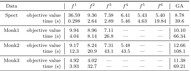
Intuitively, ramp-LPSVM can provide a sparse and robust result, if a good solution for (6) can be obtained. Hence, we first consider the optimization performance of the proposed algorithms. To evaluate them, we setµ= 1/10, σ= 1 and use the four data sets for which the training data are provided. The result of ramp-LPSVM is sparse, we hence use ˆα = 0, which is optimal when µ is large sufficiently, as the initial solution. When ˆα = 0, simply calculating shows that ˆb = 1 is optimal to (6) if there are more training data in class +1 than in class−1 (#{i:yi = 1} ≥#{i:yi =−1}). Otherwise, we set ˆb=−1. From ˆα,ˆb, we apply Algorithm 2 to minimize (6). Basically, Algorithm 2 in turn applies DC programming for local minimization and hill detouring for escaping local optima. In Table 2, we report the objective values of the obtained local optima and the corresponding computation time. The superscript indicates the sequence andf1 is the result of Algorithm 1.
Data f1 f2 f3 f4 f5 f6 GA
Spect objective value 36.59 9.36 7.38 6.41 5.43 5.40 8.78 time (s) 0.298 2.64 2.89 5.46 4.63 19.84 39.6 Monk1 objective value 9.94 8.96 7.11 — — — 10.10
time (s) 4.04 8.14 26.8 — — — 66.34 Monk2 objective value 9.17 8.24 7.31 5.48 — — 12.66 time (s) 12.3 20.9 43.1 43.5 — — 108.1 Monk3 objective value 4.92 4.02 — — — — 11.38 time (s) 3.93 32.7 — — — — 69.21
Table 2: Global Search Performance of Algorithm 2 (δ= 10−6, ε= 10−6, Kstep= 50)
computation time for hill detouring is also small, which means that the performance of Algorithm 2 is not sensitive to the initial solution. To evaluate the global search capability, we also use the Genetic Algorithm (GA) toolbox developed by Chipperfield et al. (1994). The result of GA is random and we run GA algorithm repeatedly in the similar computing time of Algorithm 2. Then we select the best one and report it in Table 2. The comparison illustrates the global search capability of Algorithm 2. The basic elements of Algorithm 1 and Algorithm 2 are both to iteratively solve LPs. For large-scale problems, some fast methods for LP, especially the techniques designed for LPSVM by Bradley and Mangasarian (2000), Fung and Mangasarian (2004), and Mangasarian (2006), are applicable to speed up the solving procedure, which can be potential future work for ramp-LPSVM.
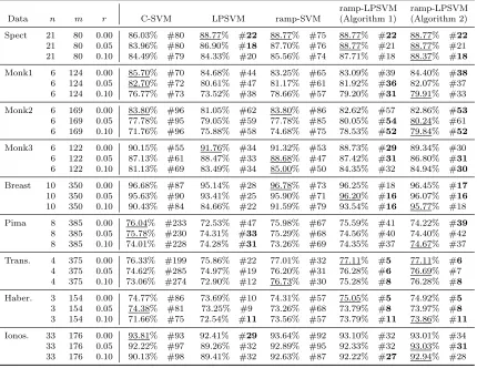
In the experiments above, the proposed algorithms show good minimization capability for ramp-LPSVM (6). Then one can expect good performance of the proposed model and algorithms, according to the robustness, sparsity, and other statistical properties discussed in Section 3. For each training set, we randomly select some data from class−1 and change their labels to be +1. The ratio of the outliers, denoted byr, is set to ber = 0.0,0.05,0.10. Based on the contaminated training set, we use C-SVM, LPSVM (5), ramp-SVM (11), and ramp-LPSVM (6) (solved by Algorithm 1 and Algorithm 2, respectively) to train the classifier and calculate the classification accuracy on the testing data. The above process is repeated 10 times. The average testing accuracy and the average number of support vectors (the corresponding|αi|is larger than 10−6) are reported in Table 3, where the data dimension n and the size of training data m are reported as well. The best results in the view of classification accuracy are underlined and the sparsest results are given in bold.
From Table 3, we observe that when there are no outliers, C-SVM performs well and LPSVM also provides good classifiers. The number of support vectors of LPSVM is always smaller than that of C-SVM, which relates to the property of `1 minimization. With an
increasing number of outliers, the accuracy of C-SVM and LPSVM decreases. In contrast, the results of ramp-SVM and ramp-LPSVM are more stable, showing the robustness of the ramp loss. The ramp loss also brings some sparsity, since when yif(xi) ≥ 0, the ramp loss gives a constant penalty, which corresponds to a zero dual variable. The proposed ramp-LPSVM consists of the `1-penalty and the ramp loss, both of which can enhance the
sparsity. Hence, the sparsity of the result of ramp-LPSVM is significant. Comparing the two algorithms for ramp-LPSVM, we find that Algorithm 2, which pursues a global solution, results in a more robust classifier. But the computation time of Algorithm 2 is significantly larger, as illustrated in Table 2. Generally, if there are heavy outliers and plenty allowable computation time, it is worth considering Algorithm 2 to find a good classifier. Otherwise, solving ramp-LPSVM by Algorithm 1 is a good choice.
5. Conclusion
In this paper, we proposed a robust classification method, called ramp-LPSVM. It consists of the`1-penalty and the ramp loss, which correspond to sparsity and robustness, respectively. The consistency and error bound for ramp-LPSVM have been discussed. Ramp-LPSVM trains a classifier by minimizing the ramp loss together with the`1-penalty, both of which are
ramp-LPSVM ramp-LPSVM Data n m r C-SVM LPSVM ramp-SVM (Algorithm 1) (Algorithm 2) Spect 21 80 0.00 86.03% #80 88.77% #22 88.77% #75 88.77% #22 88.77% #22 21 80 0.05 83.96% #80 86.90% #18 87.70% #76 88.77% #21 88.77% #21 21 80 0.10 84.49% #79 84.33% #20 85.56% #74 87.71% #18 88.37% #18 Monk1 6 124 0.00 85.70% #70 84.68% #44 83.25% #65 83.09% #39 84.40% #38 6 124 0.05 82.70% #72 80.61% #47 81.17% #61 81.92% #36 82.07% #37 6 124 0.10 76.77% #73 73.52% #38 78.66% #57 79.20% #31 79.91% #33 Monk2 6 169 0.00 83.80% #96 81.05% #62 83.80% #86 82.62% #57 82.86% #53 6 169 0.05 77.78% #95 79.05% #59 77.78% #85 80.05% #54 80.24% #61 6 169 0.10 71.76% #96 75.88% #58 74.68% #75 78.53% #52 79.84% #52 Monk3 6 122 0.00 90.15% #55 91.76% #34 91.32% #53 88.73% #29 89.34% #30 6 122 0.05 87.13% #61 88.47% #33 88.68% #47 87.42% #31 86.80% #31 6 122 0.10 81.13% #69 83.49% #34 85.00% #50 84.35% #32 84.94% #30 Breast 10 350 0.00 96.68% #87 95.14% #28 96.78% #73 96.25% #18 96.45% #17 10 350 0.05 95.63% #90 93.41% #25 95.90% #71 96.20% #16 96.07% #16 10 350 0.10 90.43% #84 84.66% #22 91.59% #79 93.54% #16 95.77% #18 Pima 8 385 0.00 76.04% #233 72.53% #47 75.98% #67 75.59% #41 74.22% #39 8 385 0.05 75.78% #230 74.31% #33 75.29% #68 74.56% #40 74.40% #42 8 385 0.10 74.01% #228 74.28% #31 73.26% #69 74.35% #37 74.67% #37 Trans. 4 375 0.00 76.33% #199 75.86% #22 77.01% #32 77.11% #5 77.11% #6
4 375 0.05 74.62% #285 74.97% #19 76.20% #31 76.28% #6 76.69% #7 4 375 0.10 73.06% #274 72.90% #12 76.73% #30 75.28% #8 76.28% #8 Haber. 3 154 0.00 74.77% #86 73.69% #10 74.31% #57 75.05% #5 74.92% #5 3 154 0.05 74.38% #81 73.25% #9 73.26% #68 73.79% #8 73.97% #8 3 154 0.10 71.66% #75 72.54% #11 73.56% #57 73.79% #11 73.86% #11 Ionos. 33 176 0.00 93.81% #93 92.41% #29 93.64% #92 93.10% #32 93.01% #34 33 176 0.05 92.22% #97 89.26% #32 92.89% #95 92.33% #32 93.03% #31 33 176 0.10 90.13% #98 89.41% #32 92.63% #87 92.22% #27 92.94% #28
proposed. The proposed algorithms have good optimization capability and ramp-LPSVM has shown robustness and sparsity in numerical experiments.
Acknowledgments
The authors are grateful to the anonymous reviewers for insightful comments.
This work was supported in part by the scholarship of the Flemish Government; Research Council KUL: GOA/11/05 Ambiorics, GOA/10/09 MaNet, CoE EF/05/006 Optimization in Engineering (OPTEC), IOF-SCORES4CHEM, several PhD/postdoc & fellow grants; Flemish Government: FWO: PhD/postdoc grants, projects: G0226.06 (cooperative systems and optimization), G.0302.07 (SVM/Kernel), G.0320.08 (convex MPC), G.0558.08 (Robust MHE), G.0557.08 (Glycemia2), G.0588.09 (Brain-machine) research communities (WOG: ICCoS, ANMMM, MLDM); G.0377.09 (Mechatronics MPC), G.0377.12 (Structured mod-els), IWT: PhD Grants, Eureka-Flite+, SBO LeCoPro, SBO Climaqs, SBO POM, O&O-Dsquare; Belgian Federal Science Policy Office: IUAP P6/04 (DYSCO, Dynamical systems, control and optimization, 2007-2011); IBBT; EU: ERNSI; ERC AdG A-DATADRIVE-B, FP7-HD-MPC (INFSO-ICT-223854), COST intelliCIS, FP7-EMBOCON (ICT-248940); Contract Research: AMINAL; Other: Helmholtz: viCERP, ACCM, Bauknecht, Hoer-biger. L. Shi is also supported by the National Natural Science Foundation of China (No. 11201079) and the Fundamental Research Funds for the Central Universities of China (No. 20520133238, No. 20520131169). Johan Suykens is a professor at KU Leuven, Belgium.
Appendix A.
In this appendix, we prove Theorem 5 in Section 2. First, we bound the offset by the following lemma.
Lemma 7 For any µ > 0, m ∈ N, and z = {xi, yi}mi=1, we can find a solution (fz,µ∗ , b∗z,µ)
of equation (6) satisfying min1≤i≤m|fz,µ(xi)| ≤1, where fz,µ=fz,µ∗ +b∗z,µ. Hence, |b∗z,µ| ≤ 1 +kfz,µ∗ k∞.
Proof Suppose a minimizer fz,µ =fz,µ∗ +b∗z,µ of (6) satisfies
r:= min
1≤i≤m|fz,µ(xi)|=|fz,µ(xi0)|>1.
Then for each i, either yifz,µ(xi) ≥ r > 1 or yifz,µ(xi) ≤ −r < −1. We consider a function fz,µd :=fz,µ−dwith d= (r−1)sgn(fz,µ(xi0)). Then fz,µd satisfies |fz,µd (xi0)|= 1 and |fd
z,µ(xi0)| ≥ 1. When yifz,µ(xi) > 1, one can check that yifz,µd (xi) ≥ 1. Similarly, if yifz,µ(xi) < −1, one still has yifz,µd (xi) ≤ −1. Then Lramp,z(fz,µ) = Lramp,z(fz,µd ). Therefore, fd
z,µ is also a solution of equation (6) and satisfies our requirement. Now if fz,µ =fz,µ∗ +b∗z,µ satisfies
|fz,µ(xi0)|= min
1≤i≤m|fz,µ(xi)| ≤1, we then have
|b∗z,µ| ≤1 +|fz,µ∗ (xi0)| ≤1 +kf
∗
In this way, we complete the proof.
In the following, we shall always choose fz,µ as in lemma 7. According to our proof, such kind of solutions can be easily constructed even though the obtained ones from the algorithm do not meet the requirement. Next, we find a function space covering fz,µ when z runs over all possible samples.
Lemma 8 For every µ >0, we have fz,µ∗ ∈ HK and
kfz,µ∗ kK≤κΩ(fz,µ∗ )≤ κ µ,
where κ= supx,y∈Xp|K(x, y)|.
Proof It is trivial thatfz,µ∗ ∈ HK. By the reproducing property (see Aronszajn, 1950), for
fz,µ∗ =Pm
i=1α∗i,zyiK(x, xi),
kfz,µ∗ kK=
m
X
i,j=1
α∗i,zα∗j,zK(xi, xj)
1/2 ≤κ
m
X
i,j=1
αi,zαj,z
1/2
=κΩ(fz,µ∗ ).
Due to the definition of fz,µ∗ , we have
Rramp,z(fz,µ) +µΩ(fz,µ∗ )≤ Rramp,z(0) +µΩ(0)≤1. This gives Ω(fz,µ∗ )≤ 1
µ, and completes the proof.
From Lemma 7, Lemma 8 and the relation
kfk∞≤κkfkK, ∀f ∈ HK,
we know thatfz,µ lies in
Fµ=
f =f∗+b∗ :kf∗kK≤
κ
µ and |b
∗| ≤1 +κ2
µ
. (28)
Now we are in the position to prove the main theorem in Section 2. Our analysis mainly focus on estimating the sample error S(m, µ, λ).
Proof of Theorem 5. We fist estimate RLramp,z(fλ)− RLramp,ρ(fλ) by considering the random variable ςi defined by (19) with f = fλ. As Lramp : R → [0,1], there holds |ςi−Eςi| ≤2. Then by the Hoeffding inequality (see, e.g., Cucker and Zhou, 2007, Corollary 3.6), with probability at least 1−δ/2, we have
RLramp,z(fλ)− RLramp,ρ(fλ)≤
s
8 log2δ
For the term RLramp,ρ(fz,µ) − RLramp,z(fz,µ), note that fz,µ varies with samples. In order to obtain the corresponding upper bound, we shall apply the uniform concentration inequality to the function setFµ. One can directly use Theorem 8 in Bartlett and Mendelson (2003) to deal with this term and find with probability at least 1−δ/2,
RLramp,ρ(fz,µ)− RLramp,z(fz,µ)≤EzEσ
"
sup g∈F˜
2 m m X i=1
σig(xi, yi)
# + s
8 log4δ
m (30)
where ˜F := {(x, y)→Lramp(yf(x))−Lramp(0) :f ∈ F } and σ1,· · ·, σm are independent uniform {−1,+1}-valued random variables. As the ramp loss is Lipschitz with constant 1, we further bound the first term in the right-hand side by the result of Bartlett and Mendelson (2003, Theorem 12) as
EzEσ
"
sup g∈F˜
2 m m X i=1
σig(xi, yi)
#
≤ 2EzEσ
" sup f∈F 2 m m X i=1
σif(xi)
#
≤ 2EzEσ
"
sup
{f∗∈H
K:kf∗kK≤κµ}
2 m m X i=1
σif∗(xi)
#
+√2 m +
2κ2 µ√m
≤ 6κ 2 µ√m +
2
√ m.
Here, the last inequality is from Lemma 22 in Bartlett and Mendelson (2003). Combining the above bound and (29), (30), we then have with probability at least 1−δ,
S(m, µ, λ)≤(2 +η)
s
8 log4δ
m +
6κ2 µ√m+
2
√ m.
Finally, we let µ= m−4ββ+1+2 and λ= m−4β1+2. Then η = µ λ =m
−4ββ+2
≤1. Therefore, by Theorem 2 and Theorem 4, we can derive the bound (20) with ˜c = 15 + 2cβ+ 6κ2. This completes our proof.
References
L.T.H. An and P.D. Tao. The DC (difference of convex functions) programming and DCA revisited with DC models of real world nonconvex optimization problems. Annals of Operations Research, 133(1):23–46, 2005.
L.T.H. An, P.D. Tao, and L.D. Muu. Numerical solution for optimization over the efficient set by DC optimization algorithms. Operations Research Letters, 19(3):117–128, 1996.
P.L. Bartlett, M.I. Jordan, and J.D. McAuliffe. Convexity, classification, and risk bounds.
Journal of the American Statistical Association, 101(473):138–156, 2006.
P.L. Bartlett and S. Mendelson. Rademacher and Gaussian complexities: risk bounds and structural results. Journal of Machine Learning Research, 3:463–482, 2003.
P.S. Bradley and O.L. Mangasarian. Massive data discrimination via linear support vector machines. Optimization Methods and Software, 13(1):1–10, 2000.
J.P. Brooks. Support vector machines with the ramp loss and the hard margin loss. Oper-ations Research, 59(2):467–479, 2011.
A. Chipperfield, P. Fleming, H. Pohlheim, and C. Fonseca. Genetic algorithm toolbox user’s guide. Research Report, 1994.
R. Collobert, F. Sinz, J. Weston, and L. Bottou. Trading convexity for scalability. In
Proceedings of the 23rd International Conference on Machine Learning, pages 201–208. ACM, 2006a.
R. Collobert, F. Sinz, J. Weston, and L. Bottou. Large scale transductive SVMs. Journal of Machine Learning Research, 7:1687–1712, 2006b.
C. Cortes and V. Vapnik. Support-vector networks.Machine Learning, 20(3):273–297, 1995.
F. Cucker and D.X. Zhou. Learning Theory: an Approximation Theory Viewpoint. Cam-bridge University Press, 2007.
K. De Brabanter, K. Pelckmans, J. De Brabanter, M. Debruyne, J.A.K. Suykens, M. Hu-bert, and B. De Moor, Robustness of kernel based regression: a comparison of iterative weighting schemes. In Proceedings of the 19th International Conference on Artificial Neural Networks, pages 100–110, 2009.
A. Frank and A. Asuncion. UCI machine learning repository, 2010. URLhttp://archive.
ics.uci.edu/ml.
R. Horst and T. Hoang. Global Optimization: Deterministic Approaches. Springer Verlag, 1996.
F.M. Fung and O.L. Mangasarian. A feature selection Newton method for support vec-tor machine classification. Computational Optimization and Applications, 28(2):185–202, 2004.
R. Horst and N.V. Thoai. DC programming: overview. Journal of Optimization Theory and Applications, 103(1):1–43, 1999.
X. Huang, J. Xu, X. Mu, and S. Wang. The hill detouring method for minimizing hinging hyperplanes functions. Computers & Operations Research, 39(7):1763–1770, 2012a.
V. Kecman and I. Hadzic. Support vectors selection by linear programming. InProceedings of the International Joint Conference on Neural Networks (IJCNN), volume 5, pages 193–198. IEEE, 2000.
Y. Lin. A note on margin-based loss functions in classification. Statistics & Probability Letters, 68(1):73–82, 2004.
O.L. Mangasarian. Exact 1-norm support vector machines via unconstrained convex differ-entiable minimization. Journal of Machine Learning Research, 7:1517–1530, 2006.
O.L. Mangasarian. Absolute value equation solution via concave minimization.Optimization Letters, 1(1):3–8, 2007.
L. Mason, J. Baxter, P.L. Bartlett, and M. Frean. Boosting algorithms as gradient descent in function space. In S.A. Solla, T.K. Leen, and K. M¨uller, editors, Advances in Neural Information Processing Systems, 12:512–518, Cambridge, MA, MIT Press, 2000.
M. Porembski. Cutting planes for low-rank-like concave minimization problems. Operations Research, pages 942–953, 2004.
S. Smale and D.X. Zhou. Estimating the approximation error in learning theory. Analysis and Applications, 1(1):17–41, 2003.
A. Smola, B. Sch¨olkopf, and G. R¨atsch. Linear programs for automatic accuracy control in regression In Proceedings of the 9th International Conference on Artificial Nerual Networks, No. 470, pages 575–580, 1999.
X. Shen, G.C. Tseng, X. Zhang, and W. Wong. On ψ-learning. Journal of the American Statistical Association, 98(463):724–734, 2003.
J. Shu and I.A. Karimi. Efficient heuristics for inventory placement in acyclic networks.
Computers & Operations Research, 36(11):2899–2904, 2009.
I. Steinwart. How to compare different loss functions and their risks. Constructive Approx-imation, 26(2):225–287, 2007.
I. Steinwart and A. Christmann. Support Vector Machines. New York: Springer, 2008.
J.A.K. Suykens and J. Vandewalle. Least squares support vector machine classifiers. Neural Processing Letters, 9(3):293–300, 1999.
J.A.K. Suykens, T. Van Gestel, J. De Brabanter, B. De Moor, and J. Vandewalle. Least Squares Support Vector Machines. World Scientific, Singapore, 2002.
V. Vapnik. Statistical Learning Theory. Wiley, New York, 1998.
K. Wang, P. Zhong, and Y. Zhao. Training robust support vector regression via DC program.
Journal of Information and Computational Science, 7(12):23852394, 2010.
Y. Wu and Y. Liu. Robust truncated hinge loss support vector machines. Journal of the American Statistical Association, 102(479):974–983, 2007.
A.L. Yuille and A. Rangarajan. The concave-convex procedure. Neural Computation, 15(4): 915–936, 2003.
T. Zhang. Statistical analysis of some multi-category large margin classification methods.
Journal of Machine Learning Research, 5:1225–1251, 2004.
Y. Zhao and J. Sun. Robust support vector regression in the primal. Neural Networks, 21(10): 1548–1555, 2008.