GPstuff: Bayesian Modeling with Gaussian Processes
Jarno Vanhatalo∗ [email protected]
Department of Environmental Sciences University of Helsinki
P.O. Box 65
FI-00014 Helsinki, Finland
Jaakko Riihim¨aki [email protected]
Jouni Hartikainen [email protected]
Pasi Jyl¨anki [email protected]
Ville Tolvanen [email protected]
Aki Vehtari [email protected]
Department of Biomedical Engineering and Computational Science Aalto University School of Science
P.O. Box 12200
FI-00076 Aalto, Finland
Editor:Balazs Kegl
Abstract
The GPstuff toolbox is a versatile collection of Gaussian process models and computational tools required for Bayesian inference. The tools include, among others, various inference methods, sparse approximations and model assessment methods.
Keywords: Gaussian process, Bayesian hierarchical model, nonparametric Bayes
1. Introduction
Gaussian process (GP) prior provides a flexible building block for many hierarchical Bayesian mod-els (Rasmussen and Williams, 2006). GPstuff (v4.1) is a versatile collection of computational tools for GP models and it has already been used in several published projects, for example, in epidemiol-ogy, species distribution modeling and building energy usage modeling (see Vanhatalo et al., 2013, and project web pages for references). GPstuff combines models and inference tools in a modular format. It also provides various sparse GP models and methods for model assessment. The tool-box is compatible with Unix and Windows Matlab (at least r2009b or later). Most features work also with Octave (tested with 3.6.4). The toolbox is available fromhttp://becs.aalto.fi/en/ research/bayes/gpstuff/and alsohttp://mloss.org/software/view/451/.
2. Implementation
In many practical GP models, the observationsy= [y1, ...,yn]T related to inputs (covariates)X= {xi= [xi,1, ...xi,d]T}ni=1are assumed to be conditionally independent given a latent function (or pre-dictor) f(x) so that the likelihood p(y|f,γ) =∏ni=1p(yi|fi,γ), where f= [f(x1), ...,f(xn)]T,
torizes over cases. The latent function is given a GP prior, f ∼GP(m(x|φ),k(x,x′|θ))which is defined by the mean and covariance function,m(x|φ) andk(x,x′|θ)respectively. The parameters, ϑ={γ,φ,θ}, are given a hyperprior after which the posterior p(f|y,X)is approximated and used for prediction. Most of the models in GPstuff follow the above single latent dependency, but there are also models where each factor depends on multiple latent values.
We illustrate the construction and inference of a GP model with a regression example. First, we assume yi = f(xi) +εi, εi ∼N(0,σ2), and give f(x) a GP prior with a squared exponential covariance function,k(x,x′) =σ2
seexp(||x−x′||2/2l2).
lik = lik_gaussian(’sigma2’, 0.2ˆ2); % init. the likelihood
gpcf = gpcf_sexp(’lengthScale’, 1, ’magnSigma2’, 0.2ˆ2) % init. the cov. function
gp = gp_set(’lik’, lik, ’cf’, gpcf); % init. the model struct
% Find MAP estimate of the parameters and predict to new inputs
opt=optimset(’TolFun’,1e-3,’TolX’,1e-3,’Display’,’iter’); % optimization settings
gp=gp_optim(gp,x,y,’optimf’,@fminscg,’opt’,opt); % x,y = training data
[Ef, Varf] = gp_pred(gp, x, y, xt); % xt = test inputs
The model is constructed modularly so that each mathematical function or distribution is repre-sented by an “object” style structure. The structureslikandgpcfcontain all the essential informa-tion about the likelihood and covariance funcinforma-tion such as parameter values and funcinforma-tion handles to construct a covariance matrix and its gradient with respect to the parameters. All the model blocks are collected into a GP structure constructed bygp set.
There are two lines of approach for the inference. The first assumes a Gaussian observation model which enables an analytic solution for the marginal likelihoodp(y|X,ϑ)and the conditional posterior p(f|X,y,ϑ). Using the relation p(ϑ|y,X)∝ p(y|X,ϑ)p(ϑ) the parameters, ϑ, can be optimized to the maximum a posterior (MAP) estimate or marginalized over with grid, central com-posite design (CCD), importance sampling (IS) or Markov chain Monte Carlo (MCMC) integration (Vanhatalo et al., 2010). With other observation models the marginal likelihood and the conditional posterior have to be approximated either with Laplace’s method (LA) or expectation propagation (EP) (Rasmussen and Williams, 2006). An alternative approach is to sample from the joint posterior
p(f,ϑ|X,y)with MCMC by alternating sampling fromp(f|X,y,ϑ)andp(ϑ|X,y,f).
Above,gp optimreturns a redefined model structure with parameter values optimized to their MAP estimate. Any optimizer with similar arguments to Matlab’s optimizers can be used.gp pred returns the conditional posterior predictive mean, E[f|y,X,ϑ]and variance Var[f|y,X,ϑ]at the test inputs.
Many sparse GPs have been proposed to speed up the computations with large data sets. GPstuff includes FI(T)C, PIC, SOR, DTC (Qui˜nonero-Candela and Rasmussen, 2005), VAR (Titsias, 2009), CS+FIC (Vanhatalo and Vehtari, 2008) sparse approximations, and several compactly supported (CS) covariance functions. For example, CS+FIC can be used with the following modification to the model initialization.
gpcf2 = gpcf_ppcs2(’nin’, nin, ’lengthScale’, 5, ’magnSigma2’, 1); gp = gp_set(’type’,’CS+FIC’,’lik’,lik,’cf’,{gpcf,gpcf2},’X_u’,Xu)
In the first line, a CS covariance function, piecewise polynomial of second order, is created. It is then given to the GP structure together with inducing inputs (Xu) and sparse GP type definition.
lik = lik_t(’nu’, 4, ’sigma2’, 10, ’nu_prior’, prior_logunif);
gp = gp_set(’lik’, lik, ’cf’, gpcf, ’jitterSigma2’, 1e-6, ’latent_method’, ’EP’);
Here we set explicitly the prior for the degrees of freedom parameter,νin the Student-tdistribution, add jitter on the diagonal of the covariance matrix and define EP as the means to approximate the marginal likelihood.
GPstuff has wide variety of observation models (see Table 1) of which we want to highlight im-plementations of recently proposed multinomial probit with EP (Riihim¨aki et al., 2013) and logistic GP density estimation and regression with Laplace approximation (Riihim¨aki and Vehtari, 2012).
The constructed models could be compared, for example, with deviance information criterion (DIC), widely applicable information criterion (WAIC), leave-one-out or k-fold cross-validation (LOO/kf-CV) (Vehtari and Ojanen, 2012) with functionsgp dic,gp waic,gp loopredandgp kfcv.
New models can be implemented by modifying the existing model blocks, such as covariance functions. Adding new inference methods is more laborious since they require summaries from model blocks which may not be provided by the current version of GPstuff. A thorough introduction to GPstuff is provided by demo programs and Vanhatalo et al. (2013).
3. Related Software
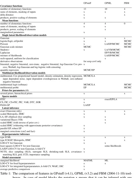
Perhaps the best known GP software packages are the Gaussian processes for Machine Learn-ing (GPML) (Rasmussen and Nickisch, 2010) and the flexible Bayesian modellLearn-ing (FBM) (Neal, 1998). Overviews of alternatives are provided by the Gaussian processes website (http://www. gaussianprocess.org/) and the R Archive Network (http://cran.r-project.org/). The main advantage of GPstuff over the other GP software is its versatile collection of models and computational tools. Its most important features and comparison to GPML and FBM are presented in Table 1. GPstuff project was started in 2006 based on the MCMCstuff-toolbox (http://becs. aalto.fi/en/research/bayes/mcmcstuff/), which was based on Netlab (Nabney, 2001) and influenced by FBM. The INLA software (Rue et al., 2009) and the book by Rasmussen and Williams (2006) have motivated some of the technical details in GPstuff. In addition, the implementation of sparse matrix routines, used with the CS covariance functions, rely on the SuiteSparse toolbox (Davis, 2005).
Acknowledgments
GPstuff GPML FBM
Covariance functions
number of elementary functions 13 10 4
sums of elements, masking of inputs x x x
delta distance x x
products, positive scaling of elements x x
Mean functions
number of elementary functions 4 4 0
sums of elements, masking of inputs x x
products, power, scaling of elements x
marginalized parameters x
Single latent likelihood/observation models
Gaussian x x x
logistic/logit, erf/probit x x MCMC
Poisson x LA/EP/MCMC MCMC
Gaussian scale mixture MCMC MCMC
Student-t x LA/VB/MCMC
Laplacian EP/VB/MCMC
mixture of likelihoods LA/EP/MCMC
sech-squared, uniform for classification x
derivative observations for sexp covf only
binomial, negative binomial, zero-trunc. negative binomial, log-Gaussian Cox pro-cess; Weibull, log-Gaussian and log-logistic with censoring
x
quantile regression MCMC/EP
Multilatent likelihood/observation models
multinomial, Cox proportional hazard model, density estimation, density regression, input dependent noise, input dependent overdispersion in Weibull, zero-inflated negative binomial
MCMC/LA
multinomial logit (softmax) MCMC/LA MCMC
multinomial probit EP MCMC
Priors for parameters (ϑ)
several priors, hierarchical priors x x
Sparse models
FITC x exact/EP/LA
CS, FIC, CS+FIC, PIC, VAR, DTC, SOR x
PASS-GP LA/EP
Latent inference
exact (Gaussian only) x x x
scaled Metropolis, HMC x x
LA, EP, elliptical slice sampling x x
variational Bayes (VB) x
scaled HMC (with inverse of prior cov.) x
scaled HMC (whitening with approximate posterior covariance) x
parallel EP, robust EP x
marginal corrections (cm2 and fact) x
Hyperparameter inference
type II ML x x x
type II MAP, Metropolis, HMC x x
LOO-CV for Gaussian x x
least squares LOO-CV for non-Gaussian some likelihoods
LA/EP LOO-CV for non-Gaussian, k-fold CV x NUTS, slice sampling (SLS), surrogate SLS, shrinking-rank SLS,
covariance-matching SLS, grid, CCD, importance sampling
x
Model assessment
marginal likelihood MAP,ML ML
LOO-CV for fixed hyperparameters x x
LOO-CV for integrated hyperparameters, k-fold CV, WAIC, DIC x
average predictive comparison x
References
Timothy A. Davis. Algorithm 849: A concise sparse Cholesky factorization package. ACM Trans. Math. Softw., 31:587–591, 2005. ISSN 0098-3500.
Pasi Jyl¨anki, Jarno Vanhatalo, and Aki Vehtari. Robust Gaussian process regression with a Student-t
likelihood. Journal of Machine Learning Research, 12:3227–3257, 2011.
Ian T. Nabney. NETLAB: Algorithms for Pattern Recognition. Springer, 2001.
Radford Neal. Regression and classification using Gaussian process priors. In J. M. Bernardo, J. O. Berger, A. P. David, and A. P. M. Smith, editors,Bayesian Statistics 6, pages 475–501. Oxford University Press, 1998.
Joaquin Qui˜nonero-Candela and Carl Edward Rasmussen. A unifying view of sparse approximate Gaussian process regression. Journal of Machine Learning Research, 6(3):1939–1959, 2005.
Carl Edward Rasmussen and Hannes Nickisch. Gaussian processes for machine learning (GPML) toolbox. Journal of Machine Learning Research, 11:3011–3015, 2010.
Carl Edward Rasmussen and Christopher K. I. Williams.Gaussian Processes for Machine Learning. The MIT Press, 2006.
Jaakko Riihim¨aki and Aki Vehtari. Laplace approximation for logistic Gaussian process density estimation. ArXiv e-prints, (1211.0174), 2012. URLhttp://arxiv.org/abs/1211.0174.
Jaakko Riihim¨aki, Pasi Jyl¨anki, and Aki Vehtari. Nested expectation propagation for Gaussian pro-cess classification with a multinomial probit likelihood. Journal of Machine Learning Research, 14:75–109, 2013.
H˚avard Rue, Sara Martino, and Nicolas Chopin. Approximate Bayesian inference for latent Gaus-sian models by using integrated nested Laplace approximations. Journal of the Royal Statistical Society B, 71(2):1–35, 2009.
Michalis K. Titsias. Variational learning of inducing variables in sparse Gaussian processes. JMLR Workshop and Conference Proceedings, 5:567–574, 2009.
Jarno Vanhatalo and Aki Vehtari. Modelling local and global phenomena with sparse Gaussian pro-cesses. In David A. McAllester and Petri Myllym¨aki, editors,Proceedings of the 24th Conference on Uncertainty in Artificial Intelligence, pages 571–578, 2008.
Jarno Vanhatalo, Ville Pietil¨ainen, and Aki Vehtari. Approximate inference for disease mapping with sparse Gaussian processes. Statistics in Medicine, 29(15):1580–1607, 2010.
Jarno Vanhatalo, Jaakko Riihim¨aki, Jouni Hartikainen, Pasi Jyl¨anki, Ville Tolvanen, and Aki Ve-htari. Bayesian modeling with Gaussian processes using the GPstuff toolbox. ArXiv e-prints, (1206.5754), 2013. URLhttp://arxiv.org/abs/1206.5754.