Dependence, Correlation and Gaussianity in Independent Component Analysis

Dependence, Correlation and Gaussianity

in Independent Component Analysis

Jean-Franc¸ois Cardoso CARDOSO@TSI.ENST.FR

ENST/TSI 46 Rue Barrault 75634, Paris, France

Editors: Te-Won Lee, Jean-Franc¸ois Cardoso, Erkki Oja and Shun-ichi Amari

Abstract

Independent component analysis (ICA) is the decomposition of a random vector in linear com-ponents which are “as independent as possible.” Here, “independence” should be understood in its strong statistical sense: it goes beyond (second-order) decorrelation and thus involves the non-Gaussianity of the data. The ideal measure of independence is the “mutual information” and is known to be related to the entropy of the components when the search for components is restricted to uncorrelated components. This paper explores the connections between mutual information, en-tropy and non-Gaussianity in a larger framework, without resorting to a somewhat arbitrary decor-relation constraint. A key result is that the mutual information can be decomposed, under linear transforms, as the sum of two terms: one term expressing the decorrelation of the components and one expressing their non-Gaussianity.

Our results extend the previous understanding of these connections and explain them in the light of information geometry. We also describe the “local geometry” of ICA by re-expressing all our results via a Gram-Charlier expansion by which all quantities of interest are obtained in terms of cumulants.

Keywords: Independent component analysis, source separation, information geometry, mutual information, minimum entropy, non-Gaussianity, cumulant expansions

Introduction

Independent component analysis (ICA) is the decomposition of a random vector in linear com-ponents which are “as independent as possible.” This emerging technique appears as a powerful generic tool for data analysis and the processing of multi-sensor data recordings. In ICA, “inde-pendence” should be understood in its strong statistical sense: it is not reduced to decorrelation (second-order dependence) because, for the purpose of ICA, second order statistics fail to capture important features of a data set, as shown by the fact that there are infinitely many linear transforms which decorrelate the entries of a random vector.

A fascinating connection exists between maximum independence and minimum entropy: if one decides to restrict the search for linear components to components which are uncorrelated and have unit variance (this later constraint is just a normalization convention), then the objective of minimizing the mutual information is equivalent to the objective of minimizing the sum of the entropies of all components (see Section 1.2).

The aim of this contribution is to explore the connections between mutual information, entropy and non-Gaussianity in a general framework, without imposing the somewhat arbitrary decorrela-tion constraint. Our results extend the previous understanding of these connecdecorrela-tions with, in Equa-tion (17), the following key point: in ICA, mutual informaEqua-tion can be decomposed in two terms, a term measuring decorrelation between the components and a term measuring their Gaussianity. As it turns out, these connections are expressively described in the light of information geometry.

This paper is organized as follows. In Section 1, we recall the traditional definitions related to the information-theoretic objectives of ICA. In Section 2, we consider the problem of approximating the distribution of a vector by a Gaussian distribution and by a product distribution (a distribution with independent entries). This process naturally introduces the relevant information-theoretic defi-nitions for independence, decorrelation and non-Gaussianity and highlights their connections. Their relevance is discussed in the context of ICA. Section 3 illuminates these results by exhibiting their underlying geometric structure in the framework of information geometry. Section 4 describes the

local (in the vicinity of Gaussian distributions) geometry in terms of cumulants. Additional

com-ments conclude the paper.

1. Information-Theoretic Objectives of ICA

This section briefly recalls the basic definitions for the objective functions considered in ICA. Throughout the paper, we consider an n-dimensional random vector Y . All the sums ∑i· · · which appear in the paper are to be read as sums∑n_i=1· · · over the entries of this vector, and similarly for the products∏i· · ·.

1.1 Mutual Information or “Dependence”

The independent component analysis (ICA) of a random vector Y , as introduced by Comon (1994), consists of finding a basis on which the coordinates of Y are “as independent as possible.” A measure of statistical independence is the Kullback-Leibler divergence (KLD) from the distribution P(Y)of

Y to the product of its marginal distributions:

I(Y)def= KP(Y),∏iP(Yi)

, (1)

where the divergence KQ,Rfrom a probability distribution Q to another distribution R is defined as

KQ,Rdef=

Z

Y

Q(y)logQ(y)

R(y)dy. (2)

if Y and Z are two n-dimensional vectors then

KP(Y),P(Z)=KP(µ+TY),P(µ+T Z) (3)

for any fixed invertible n×n matrix T and any fixed shift µ.

1.2 Decorrelation and Minimum Entropy

In practical implementations of ICA, it is sometimes preferred to determine the best linear transform of Y via a two-step approach: after mean removal, the first step is to “whiten” or to “sphere” the data and the second step is to rotate them to maximize a measure of independence. The whitening step is a simple operation by which the covariance matrix RY of Y is made equal to the identity matrix, yielding components which are uncorrelated but not necessarily independent. The rotation step keeps the covariance of Y equal to the identity, thus preserving the whiteness, hence the decor-relation of the components. This technique is sometimes referred to as the “orthogonal approach.” In the orthogonal approach, the overall transformation is often explicitly obtained as the product of a whitening matrix by an orthogonal matrix but for the purpose of analysis, there is no need to consider the specific practical implementation; an equivalent formulation is to say that the partic-ular measure of independence (used in the second step) is to be optimized “under the whiteness constraint,” that is, over all the linear transforms such that RY is the identity matrix.

By turning the logarithm of the ratio in (2) into a difference of logarithms, one readily finds that

I(Y) =

∑

i

H(Yi)−H(Y), (4)

where H(·)denotes Shannon’s “differential entropy” for continuous random variables:

H(Y) =−

Z

YPY

(y)log PY(y)dy.

Recall that applying a linear transform T to a vector adds a term log|det T|to its entropy. It follows that the entropy H(Y)remains constant under the whiteness constraint because all the white versions of Y are rotated versions of each other and because log|det T|=0 if T is an orthogonal matrix.

Thus the dependence (or mutual information) I(Y)admits a very interesting interpretation under the whiteness constraint since it appears by (4) to be equal, up to the constant term H(Y), to the sum of the marginal entropies of Y . In this sense, ICA is a minimum entropy method under the whiteness

constraint. It is one purpose of this paper to find out how this interpretation is affected when the

whiteness constraint is relaxed.

2. Dependence, Correlation and Gaussianity

2.1 Product Approximation and Dependence

The divergence KP(Y),∏iQi

from the distribution P(Y)of a given n-vector to the product of any

n scalar probability distributions Q1, . . . ,Qncan be decomposed as:

KP(Y),∏iQi

=KP(Y),∏iP(Yi)

+K∏iP(Yi),∏iQi

. (5)

This classic property is readily checked by direct substitution of the distributions into the definition of the KL divergence; its geometric interpretation as a Pythagorean identity is given at Section 3.

The first divergence on the right hand side of (5) is the dependence (or mutual information)

I(Y)defined in Equation (1). The second divergence on the right hand side involves two product densities so that it decomposes into the sum of the divergences between the marginals:

K∏iP(Yi),∏iQi

=∑iKP(Yi),Qi

.

It follows that the KLD from a distribution P(Y)to any product distribution can be read as

KP(Y),∏iQi

=I(Y) +∑iKP(Yi),Qi

. (6)

This decomposition shows that KP(Y),∏iQi

is minimized with respect to the scalar distributions

Q1, . . . ,Qn by taking Qi=P(Yi)for i=1, . . . ,n because this choice ensures that K

P(Yi),Qi

=0 which is the smallest possible value of a KLD. Thus, the product distribution

PP(Y)def=

∏

i

P(Yi)

appearing in Definition (1) is the best “product approximation” to P(Y)in that it is the distribution with independent components which is closest to P(Y)in the KLD sense.

2.2 Gaussian Approximation and Non-Gaussianity

Besides independence, another distributional property plays an important role in ICA: normality. Denoting

N

(µ,R) the Gaussian distribution with mean µ and covariance matrix R, the divergence

KP(Y),

N

(µ,R)from the distribution of a given n-vector Y to a Gaussian distribution

N

(µ,R)

can be decomposed into

KP(Y),

N

(µ,R)=KP(Y),

N

(EY,RY)

+K

N

(EY,RY),

N

(µ,R)

, (7)

where RYdenotes the covariance matrix of Y . Just as in (5), this decomposition is readily established by substitution of the relevant densities in the definition of the KLD or, again, as an instance of a general Pythagorean theorem (see Section 3).

Decomposition (7) shows that KP(Y),

N

(µ,R)is minimized with respect to µ and R for µ=

EY and R=RY since this choice cancels the (non-negative) second term in Equation (7) and since the first term does not depend on µ or R. Thus,

PG(Y)def=

N

(EY,RY)

is, not surprisingly, the best Gaussian approximation to P(Y)in the KLD sense. The KL divergence from the distribution of Y to its best Gaussian approximation is taken as the definition of the (non)

Gaussianity G(Y)of vector Y :

This definition encompasses the scalar case: the non-Gaussianity of each component of Yiis

G(Yi) =K

P(Yi),

N

(EYi,var(Yi))

. (9)

For further reference, we note that the non-Gaussianity of a vector is invariant under invertible affine transforms. Indeed if vector Y undergoes an invertible affine transform: Y →µ+TY (where T is a

fixed invertible matrix and µ is a fixed vector), then its best Gaussian approximation undergoes the same transform so that

G(µ+TY) =G(Y). (10)

This is because the KLD itself is invariant under affine transforms as recalled in Equation (3).

2.3 Gaussian-Product Approximation and Correlation

Looking forward to combining the results of the previous two sections, we note that the product approximation to P(Y)can be further approximated by its Gaussian approximation and vice versa. The key observation is that the same result is obtained along both routes: the Gaussian approxi-mation to the product approxiapproxi-mation, on one hand, and the product approxiapproxi-mation to the Gaussian approximation, on the other hand, are readily seen to be the same distribution

PP∧G(Y)def=

N

(EY,diag(RY)),

where diag(·) denotes the diagonal matrix with the same diagonal elements as its argument. The KLD from P(Y)to its best Gaussian-product approximation PP∧G(Y)can be evaluated along both routes.

Along the route P(Y)→PP(Y)→PP∧G(Y), we use decomposition (6) with Qi=

N

(EYi,var(Yi)). This choice ensures that∏iQi=

N

(EY,diag(RY))and, in addition, by Definition (9), K

P(Yi),Qi

is nothing but the non-Gaussianity G(Yi)of the i-th entry of Y . Thus, property (6) yields a decom-position

KP(Y),PP∧G(Y)=I(Y) +

∑

i

G(Yi) (11)

into well identified quantities: dependence and marginal (non) Gaussianities.

Along the route P(Y)→PG(Y)→PP∧G(Y), instantiating property (7) with µ=EY and R=

diag(RY)yields

KP(Y),PP∧G(Y)=G(Y) +C(Y), (12)

where we use Definition (8) of the non-Gaussianity and where we introduce the correlation C(Y)of a vector Y , defined as

C(Y)def= K

N

(EY,RY),

N

(EY,diag(RY))

=KPG(Y),PP∧G(Y). (13)

The scalar C(Y) appears as an information-theoretic measure of the overall correlation between the components of Y . In particular, C(Y)≥0 with equality only if the two distributions in (13) are identical, i.e. if RY is a diagonal matrix. The correlation C(Y) has an explicit expression as a function of the covariance matrix RY: standard computations yields

C(Y) =1

2off(RY) where off(R) def

The function R→off(R) is sometimes used as a measure of diagonality of a positive matrix R. This correlation C(Y)is invariant under the shifting or rescaling of any entry of Y . If we define a standardized vector ˜Y by

˜

Y =diag(RY)−

1

2(Y−EY) or Y˜_i= (Y_i−EY_i)/var 1

2(Y_i), (14)

then C(Y) =C(_Y˜_{) so that the correlation actually depends on the covariance matrix only via the}

correlation matrix R_Y˜ of Y . We have C(Y) = 1₂off(R_Y˜). In particular, if Y is a weakly correlated

vector, i.e. RY˜ is close to the identity matrix, a first order expansion yields

C(Y)≈1

2_1≤i<

∑

_j≤nρ 2

i j where ρi j

def

= E ˜YiY˜j=corr(Yi,Yj). (15)

In general, however, our definition of correlation is not a quadratic function of the correlation coef-ficientsρi j. For instance, in the simple case n=2, one finds C(Y) =−1

2log(1−ρ 2 12). 2.4 Dependence, Correlation and Non-Gaussianity

Two different expressions of the Kullback divergence from the distribution P(Y)of a random vec-tor to its closest Gaussian-product approximation PP∧G(Y) have been obtained at equations (11) and (12). Equating them, we find a general relationship between dependence, correlation and non Gaussianity:

I(Y) +

∑

i

G(Yi) =G(Y) +C(Y). (16)

We note that all the quantities appearing in (16) are invariant under the rescaling or shifting of any of the entries of Y .

When Y is a Gaussian vector, then G(Y) =0 and its marginals are also Gaussian: G(Yi) =0 for i=1,n. In this case, property (16) reduces to I(Y) =C(Y), that is, the obvious result that the dependence is measured by the correlation in the Gaussian case. Relation (16) also shows that, for a non-Gaussian vector, the difference I(Y)−C(Y)between dependence and correlation is equal to the difference between the joint non-Gaussianity G(Y)and the sum of the marginal non-Gaussianities (more about this difference in Section 3.4).

The most significant insight brought by property (16) regards the ICA problem in which the dependence I(Y) is to be minimized under linear transforms. We saw in Equation (10) that the non-Gaussianity G(Y)is invariant under linear transforms so that property (16) also yields

I(Y) =C(Y)−

∑

i

G(Yi) +cst, (17)

where “cst” is a term which is constant over all linear transforms of Y (and actually is nothing but

G(Y)). Hence, the issue raised in the introduction receives a clear and simple answer:

Minimizing under linear transforms the dependence I(Y)between the entries of a vec-tor Y is equivalent to optimizing a criterion which weights in equal parts the correlation

2.5 Objective Functions of ICA

Expression (17) nicely splits dependence into correlation and non-Gaussianity. It lends itself to a simple generalization. Let w be a positive number and consider the weighted criterion

φw(Y) =wC(Y)−

∑

i

G(Yi) (18)

to be optimized under linear transforms of Y . Different weights correspond to different variations around the idea of ICA:

• For w=1, the minimization ofφw under linear transforms is equivalent to minimizing the dependence I(Y).

• For w=0, the criterion is a sum of uncoupled criteria and the problem boils down to inde-pendently finding directions in data space showing the maximum amount of non Gaussianity. This is essentially the rhetoric of projection pursuit, initiated by Friedman and Tukey (1974) and whose connections to ICA have long been noticed and put to good use for justifying sequential extraction of sources as in the fastICA algorithm (see Hyv ¨arinen, 1998).

• For w→∞, the criterion is dominated by the correlation term C(Y). Thus, for w large enough, φw(Y)is minimized by linear transforms such that C(Y) is arbitrarily close to 0. The latter condition leaves many degrees of freedom; in particular, since all the quantities in (18) are scale invariant, one can freely impose var(Yi) =1 for i=1,n. These normalizing condi-tions together with C(Y) =0 are equivalent to enforcing the whiteness of Y . Thus, for w large enough, the unconstrained minimization ofφw(y)is equivalent to maximizing the sum ∑iG(Yi) of the marginal non-Gaussianities under the whiteness constraint. This objective of maximal marginal non-Gaussianity and the objective of minimum marginal entropy re-called in Section 1.2 should be identical since they both stem from the minimum dependence objective under the whiteness constraint. Indeed, it is easily seen that if var(Yi) =1 then

H(Yi) =−G(Yi) +1₂log 2πe.

3. Geometry of Dependence

This section shows how the previous results fit in the framework of information geometry. Informa-tion geometry is a theory which expresses the concepts of statistical inference in the vocabulary of differential geometry. The “space” in information geometry is a space of probability distributions where each “point” is a distribution. In the context of ICA, the distribution space is the set of all possible probability distributions of an n-vector. Two subsets (or manifolds) will play an important role: the Gaussian manifold, denoted as

G

, is the set of all n-variate Gaussian distributions and the

product manifold, denoted as

P

, is the set of all n-variate distributions with independent

compo-nents. Statistical statements take a geometric flavor. For instance, “Y is normally distributed” is restated as “the distribution of Y lies on the Gaussian manifold” or “P(Y)∈

G

.”

geometric view point has already been used in ICA to analyze contrast functions (see Cardoso, 2000) and estimating equations (see Amari and Cardoso, 1997).

3.1 Simple Facts from Information Geometry

We start by some simple notions of information geometry. For the sake of exposition, technical complications are ignored. This will be even more true in Section 4.

Exponential families. The product manifold

P

and the Gaussian manifold

G

both share an im-portant property which makes geometry simple: they are exponential families of probability dis-tributions. An exponential family has the characteristic property that it contains the exponential

segment between any two of its members. The exponential segment between two distributions with

densities p(x)and q(x)(with respect to some common dominating measure) is the one-dimensional set of distributions with densities

p_α(x) =p(x)1−αq(x)αe−ψ(α), 0≤α≤1,

whereψ(α) is a normalizing factor such that pα sums to 1. Thus, the log-density of exponential families has a simple form. An L-dimensional exponential family of distributions can be parame-terized by a setα= (α1, . . . ,αL)of real parameters as

log p(x;α) =log g(x) +

L

∑

l=1

αlSl(x)−ψ(α), (19)

where g(x) is some reference measure (not necessarily a probability measure), Sl(x) are scalar functions of the variable andψ(α)is such thatR p(x;α)dx=1.

The Gaussian manifold

G

is a p-dimensional exponential manifold with L=n+n(n+1)/2: one can take g(x)to be any n-variate Gaussian distribution and

{Sl(x)}Ll=1={xi|1≤i≤n} ∪ {xixj|1≤i≤ j≤n}. (20) The product manifold

P

also is an exponential manifold but it is infinite dimensional since the marginal distributions can be freely chosen. Similarly to Equation (19), any distribution p(x)of

P

can be given a log-density in the form

log p(x) =log g(x) +

n

∑

i=1

ri(xi)−ψ(r1, . . . ,rn), (21)

where g(x)is some product distribution of

P

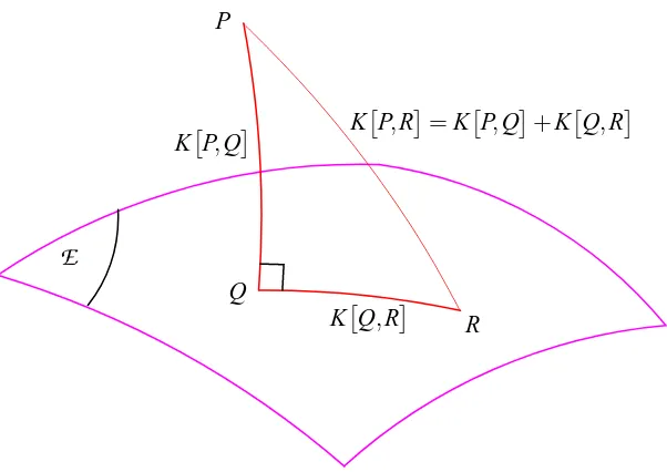
and each functions ri(·)can be freely chosen (as long as the sum of its exponential remains finite). If g(x) is the Lebesgue measure and the ri(xi) are log-densities, thenψ=0.

A Pythagorean theorem. Exponential families play a central role in statistics as well as in in-formation geometry where they behave to some extent like “flat manifolds,” (see Amari, 1985). In particular, they give rise to a Pythagorean theorem illustrated by Figure 1. This theorem states that for an exponential family

E

of distributions and for any distribution P (not necessarily in

E

), there is a unique distribution Q of

E

such that the divergence from P to any distribution R of

E

decomposes as

E

P

Q

R

KP,Q

KQ,R

KP,R=KP,Q+KQ,R

Figure 1: The Pythagorean theorem in distribution space. The distribution Q closest to P in an exponential family

E

is the “orthogonal projection” of P onto

E

. The divergence KP,R

from P to any other distribution R of

E

can be decomposed into KP,R=KP,Q+ KQ,R, i.e. a normal part and a tangent part.

This decomposition shows that Q is the closest distribution to P in

E

in the KLD sense since KQ,R

reaches its minimum value of 0 for Q=R. Thus, Q can be called the “orthogonal projection” of P

onto

E

and decomposition (22) should be read as a Pythagorean theorem in distribution space with the KL divergence being the analogue of a squared Euclidean distance.

An important remark is that all distributions P projecting at point Q in an exponential manifold characterized by functions Sl(x)as in (19) are such that

EPSl(x) =EQSl(x) l=1, . . . ,p.

In particular, all distributions projecting at a given point on

G

have the same first and second order moments according to (20) and all distributions projecting at a given point on

P

have the same marginal distributions. This is the information-geometric interpretation of the results recalled in Sections 2.1 and 2.2.

On “lengths.” We offer a word of warning about the Pythagorean theorem and information ge-ometry in general: strictly speaking, the KL divergence KP,Qfrom distribution P to distribution

Q should not be interpreted as a (squared) “length” because the divergence is not a distance (it is

P(Y)

PP(Y) =

∏iP(Yi)

PG(Y) =

N

(EY,RY)

PP∧G(Y) =

N

(EY,diag(RY))

I(Y)

dependence

∑iG(Yi)

marginal Gaussianities

C(Y)

correlation

Gaussianity

G(Y)

P

G

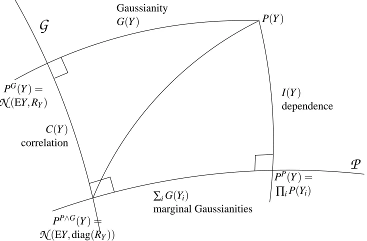
Figure 2: The geometry of decomposition (16) in distribution space (information geometry). The property I(Y) +∑iG(Yi) =G(Y) +C(Y)is found by applying a Pythagorean theorem to two right-angled triangles with a common hypotenuse: the segment from P(Y)to its best Gaussian-product approximation

N

(diag(RY)).

3.2 Geometry of Dependence and Non-Gaussianity

Information geometry allows to represent the various relations encountered so far in a single syn-thetic picture (see Figures 2 and 3). Again, each “point” in the figure is a probability distribution of an n-vector. The product manifold

P

, and the Gaussian manifold

G

are shown as one-dimensional manifolds but their actual dimensions are (much) larger, indeed.

As seen in Section 2, the minimum KL divergence from an arbitrary distribution P(Y) to the product manifold and to the Gaussian manifold is reached at points PP(Y) =∏iP(Yi) and

PG(Y) =

N

(EY,RY)respectively. These two distributions are the “orthogonal projections” of P(Y) onto

P

and

G

respectively. The dependence I(Y)and the non-Gaussianity G(Y)of Y are read as divergences from P(Y)to its projections and the corresponding edges are labelled accordingly. The two projections of P(Y)on each manifold are further projected onto each other manifold, reaching the point PP∧G(Y) =

N

(EY,diag(RY))in each case. The corresponding edges are labelled as C(Y) and∑iG(Yi).

The Pythagorean theorem can be applied to both triangles, taking P=P(Y)and R=PP∧G(Y) =

N

(EY,diag(RY))and appropriate values for

E

, Q as follows. On the Gaussian side, we take

E

=

G

and Q=PG_{(Y) =}

N

_(EY,R

G(Y) =0.103

∑iG(Yi) =0.029

C(Y) =0.084 I(Y) =0.158

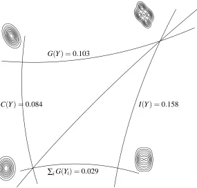
Figure 3: An example of the two-way decomposition. Kullback-Leibler divergences are expressed in “nats” and not in “bits,” i.e., they are computed using the natural logarithm.

In summary, our key result (16) relating dependence, correlation and Gaussianity admits a sim-ple geometric picture: the quantities of interest are the “lengths” of the edges of two “right-angled” triangles; these “lengths” are related because the two triangles share the same hypotenuse.

The generic picture is displayed on Figure 2; a specific example of a 2-dimensional distribution is shown on Figure 3. For P(Y) we take the distribution of Y =CS where C is an 2×2 linear transform and the entries of the 2×1 vector S are independent with bimodal (marginal) distributions. Contour plots for the densities are shown as well as the specific values of the divergences. A weak (and futile) effort has been made to have the squared lengths of the edges on the figure be roughly proportional to the corresponding KL divergences.

3.3 Some Comments

Gaussianity G(Y)reduces to marginal Gaussianity∑iG(Yi)when projecting onto the manifold

P

of independent components.

Thus correlation and marginal Gaussianity can be respectively understood as projection of the dependence on the Gaussian manifold and as projection of joint Gaussianity on the product mani-fold.

If we were dealing in Euclidean geometry, we would conclude that the projected segments have a shorter “length.” Actually, the variation of “length” is the same for both G(Y) and I(Y) since Equation (16) also reads

I(Y)−C(Y) =G(Y)−

∑

i

G(Yi), (23)

showing that the loss from full dependence I(Y) to correlation C(Y) equals the loss from joint Gaussianity G(Y)to the sum∑iG(Yi)of marginal Gaussianities. However, we are dealing with a curved geometry here: it is not true that projecting onto an exponential family always reduces the KL divergence.1 This is not even true in the specific case under investigation, as seen next.

A failed conjecture. Even though correlation is the projection of dependence onto the Gaussian manifold, the conjecture that I(Y)≥C(Y)is not true in general. A simple counter-example2_{is for} a two-dimensional Y distributed as Y =

1 1

S+σN where S is a binary random variable taking

values 1 and−1 with equal probability and N is a

N

(0,I)variable independent of S. It is not difficult to see that for small enough σ, the dependence I(Y) is close to 1 bit while the correlation C(Y)

diverges to infinity as−logσ2. Thus C(Y)>I(Y)for small enough σ, disproving the conjecture. Subsection 3.4 investigates this issue further by developing a finer geometric picture.

Location-scale invariance. Figure 2 and following show the Gaussian manifold

G

and the prod-uct manifold

P

intersecting at a single point. In fact

G

∧

P

is a 2n-dimensional manifold since it contains all uncorrelated Gaussian distributions (n degrees of freedom for the mean and n degrees of freedom for the variance of each component). These degrees of freedom correspond to location-scale transformations: Y →µ+DY with µ a fixed (deterministic) arbitrary n-vector and with D a

fixed arbitrary invertible diagonal n×n matrix. If Y undergoes such a transform, so do its product,

Gaussian and Gaussian-product approximations so that the quantities I(Y), C(Y), G(Y), and G(Yi) are invariant under location-scale transform (because of the invariance (3) of the KL divergence).

Thus the whole geometric picture is strictly invariant under location-scale changes of Y : these additional dimensions need not be represented in our figures. Each figure is a “cut” with constant location-scale parameters across the whole distribution space. All these cuts, which are orthogonal (in some sense) to the location-scale directions, show the same picture.

Orthogonality. So far, we have used the term “orthogonal” mostly in “orthogonal projection.” Figures like 2 are decorated with the symbol of a right angle at point PP_{(Y) for instance, even} though we have not defined the segment from P(Y)to PP(Y)which would be “orthogonal” to the manifold at this point. The intuitive reader may also feel that the “double Pythagoras’ used above may depend on

P

and

G

being “orthogonal” at PP∧G(Y).

Actually, the product manifold

P

and the Gaussian manifold

G

do meet orthogonally along

their intersection, the location-scale family discussed above. Unfortunately, in order to discuss this

point, one needs to define the notion of tangent plane to a statistical manifold and the notion of orthogonality in information geometry. To keep this article flowing, explaining these notions is deferred to appendix A which only contains a brief introduction to the topic. The notion of tangent plane is also used in Section 4.

Note that there is no need to prove that

P

and

G

intersect orthogonally to reach the conclu-sions of previous sections: one only has to realize that the product-Gaussian approximation and the Gaussian-product approximation to P(Y)“happen” to be identical.

3.4 Capturing Second-order and Marginal Structures

We have discussed the best approximation of an n-variate distribution by a Gaussian distribution or by an independent distribution. We now take a look at combining these two aspects.

Figures like 2 or 3 are misleading if they suggest that the distributions P(Y), PG(Y), PP(Y)and

PP∧G(Y)are somehow “coplanar.” It is in fact interesting to introduce the “plane” spanned by the product manifold

P

and the Gaussian manifold

G

. To this effect, consider the family of probability distributions for an n-vector with a log-density in the form

log p(y) =logφ(y) +

∑

i

aiyi+

∑

i j

ai jyiyj+

∑

i

ri(yi)−ψ, (24)

whereφ(y)is the n-variate standard normal distribution

N

(0,I), where ai (i=1,n) and ai j (i,j=

1,n) are real numbers, where ri(·)(i=1,n) are real functions and where ψis a number such that

R

p(y) =1. This number depends on the ai’s, on the ai j’s and on the ri(·)’s. By construction, the set of probability distributions generated by Definition (24) forms an exponential family. It contains both the Gaussian manifold

G

(characterized by ri(·) =0 for i=1,n) and the product manifold

P

(characterized by ai j=0 for 1≤i6= j≤n) (compare to (19-20) and to (21) respectively). It is actually the smallest exponential family containing both

P

and

G

; it could also be constructed as the set of all exponential segments between any distribution of

P

and any distribution of

G

. Thus, this manifold can be thought of as the “exponential span” of

P

and

G

and for this reason, it is denoted as

P

∨

G

.

Let PP∨G(Y)denote the projection of P(Y)onto

P

∨

G

, i.e.

PP∨G(Y) =arg min Q∈P∨GK

P(Y),Q(Y).

Since

P

∨

G

is an exponential family, we have yet another instance of the Pythagorean theorem:

∀R∈

P

∨

G

KP,R=KP,PP∨G+KPP∨G,R. (25)

It follows that the distribution R of

P

which minimizes KP,Ris the same as the distribution R of

P

which minimizes KPP∨G_{,R. Thus P}P∨G_{(Y)projects onto}

P

_{at the same point as P(Y), namely} at point PP(Y) =∏iPi(Yi). Similarly, PP∨G(Y)projects onto

G

at the same point as P(Y), that is, at point PG(Y) =

N

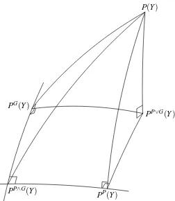
(EY,RY). It follows that PP∨G(Y)does have the same marginal distributions and the same first and second order moments as P(Y).

Our geometric picture can now be enhanced as shown on Figure 4. The figure displays the new distribution PP∨Gand also the “right angles” resulting from the projection of P(Y)onto

P

∨

G

, onto

P(Y)

PG(Y)

PP(Y)

PP∨G(Y)

PP∧G(Y)

Figure 4: Projection onto the “exponential plane”

P

∨

G

spanned by the product manifold

P

and the Gaussian manifold

G

. The projected distribution PP∨G(Y) further projects on

P

at

PP(Y) =∏iP(Yi)and on

G

at PG(Y) =

N

(EY,RY)as P(Y)itself does.

Instantiating the Pythagorean decomposition (25) with R(Y) =PP(Y) =∏iP(Yi)and with R(Y) =

PG(Y) =

N

(EY,RY)respectively yields

I(Y) = KP,PP=KP,PP∨G+KPP∨G,PP=KP,PP∨G+I(PP∨G), (26)

G(Y) = KP,PG=KP,PP∨G+KPP∨G,PG=KP,PP∨G+G(PP∨G). (27)

These identities are to be interpreted as follows: distribution PP∨G_{is the simplest approximation to}

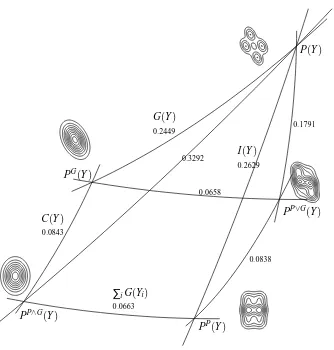
P(Y)in the sense that its log-density contains only terms as those in (24); it captures its marginal structure and its first and second order structure; it is however less dependent and more Gaussian than the original distribution P(Y)with the same quantity KP,PP∨G_{“missing” from the} depen-dence and from the (non) Gaussianity. An explicit example is displayed in Figure 5.

G(Y)

0.2449

I(Y)

0.2629

∑iG(Yi) 0.0663

C(Y)

0.0843

0.0658

0.0838 0.3292

0.1791

P(Y)

PG(Y)

PP(Y) PP∧G(Y)

PP∨G(Y)

Figure 5: Projection onto

P

∨

G

. The distribution P(Y), with Gaussianity G(Y) ≈0.2449 nats and dependence I(Y)≈0.2629 nats is approximated by PP∨G(Y) which has the same mean, same covariance and same marginal distributions as Y but reduced Gaussianity and dependence: G(PP∨G)≈0.0658 nats and I(PP∨G)≈0.0838 nats. The reduction of both quantities is KP,PP∨G≈0.1791 nats.

small enough neighborhoods. This is the case here if the divergence of P(Y)from PP∧G(Y)is small enough. In this approximation, points P, PG, PP and PP∨G can be assimilated to the vertices of a rectangle, in which case the opposite edges of the rectangle approximately have identical “lengths.”

KPP∨G,PG≈KPP,PP∧G i.e. G(PP∨G)≈

∑

i

G(Yi),

These approximations, combined with (26-27) then yields, for a weakly correlated, weakly non-Gaussian vector Y :

I(Y) ≈ C(Y) +KP,PP∨G,

G(Y) ≈

∑

i

G(Yi) +K

P,PP∨G.

Thus, in the limit of weakly correlated, weakly non-Gaussian distributions, correlation is smaller than dependence and marginal non-Gaussianity is smaller than joint non-Gaussianity by the same

positive amount KP,PP∨Gwhich measures the loss of approximating P(Y)by the simplest

distri-bution with same marginal and Gaussian structure.

Unfortunately, as shown by the counter-example of Section 3.3, this property is not true in full generality that I(Y)≥C(Y)or, equivalently by (23), that G(Y)≥∑iG(Yi).

The next section studies in more detail the “local picture” —i.e. P(Y) is close to PP∧G(Y) =

N

(EY,diag(RY))— by relying on a cumulant expansion of the KL divergence.

4. Cumulants and the Local Geometry

Cumulants and other higher order statistics have been a popular and sometimes effective tool to de-sign tractable objective functions for ICA (see for instance Comon (1994), Cardoso (1999)). They can be introduced on an ad hoc basis or as approximations to information-theoretic objective func-tions such as those discussed above. This section shows how the story of previous secfunc-tions is told in the language of cumulants.

We look at the local geometry i.e. when the distribution of Y is in the neighborhood of PP∧G(Y) =

N

(EY,diag(RY)), that is, when Y is weakly correlated and weakly non-Gaussian. In this limit, the various statistical manifolds can be approximated by their respective tangent planes and the Kull-back divergence can be approximated by a quadratic measure: the geometry becomes Euclidean. This section is organized as follows: we recall the notion of tangent plane to a statistical model and how the Kullback divergence becomes a quadratic distance in the tangent plane. Next, the tangent plane is equipped with an orthogonal basis: the (multi-dimensional) Hermite polynomials stemming from the Gram-Charlier expansion. On this basis, the coordinates of a distribution are its cumulants. Combining all these results, we give cumulant-based expansions for the dependence I(Y), the Gaus-sianity G(Y)and the correlation C(Y)allowing us to complement the global non-Euclidean picture of previous sections with a more detailed local Euclidean picture.

Tangent plane. We give an informal account of the construction of the tangent plane to a statistical model. Let n(x)and p(x)be probability densities. Then, the random variable

e(x) = p(x)

n(x)−1 (28)

has zero-mean under n(x)sinceRn(x)e(x)dx=R(p(x)−n(x))dx=1−1=0. If p(x)is “close to

If p(x)and q(x)denote two distributions close to n(x), the second-order expansion of the KLD in powers of ep(x) =p(x)/n(x)−1 and of eq(x) =q(x)/n(x)−1 is found to be

Kp,q≈Kn

p,qdef= 1

2

Z _q(x)

n(x)− p(x) n(x)

2

n(x)dx=1

2En{(eq(x)−ep(x))

2_{}. (29)} This is a quadratic form in ep−eq: the tangent space is equipped with this Euclidean metric, which is the approximation of the KLD in the vicinity of n.

Gram-Charlier expansion. A (multivariate) Gram-Charlier expansion of p(x)around a reference distribution n(x)is an expansion of p(x)in the form

ep(x) =

p(x)

n(x)−1=

∑

_i ηih

i_{(x) +} 1

2!

∑

_{i j} ηi jh

i j_{(x) +} 1

3!

∑

_{i jk}ηi jkh

i jk_{(x) +· · ·, (30)}

where theη’s are coefficients and the h’s are fixed functions of x which depend on the choice of the reference point n(x). For this expression of the Gram-Charlier expansion and multivariate Hermite polynomials, see McCullagh (1987).

For our purposes, we only need to consider a simple case in which the reference distribution is the standard n-variate normal density:

n(x) =φ(x)def= (2π)−n/2exp(−kxk2_{/2). (31)}

The h functions in the Gram-Charlier expansion are the multidimensional Hermite polynomials:

hi(x) = xi, (32)

hi j(x) = xixj−δi j, (33)

hi jk(x) = xixjxk−xiδjk[3], (34)

hi jkl(x) = xixjxkxl−xixjδkl[6] +δi jδkl[3], (35)

and so on, whereδi j is the Kronecker symbol. The bracket notation means that the corresponding term should be repeated for all the relevant index permutations. For instance: xiδjk[3]stands for

xiδjk+xjδki+xkδi j and xixjδkl[6]stands for all the partitions of the set(i,j,k,l)into three blocks according to the pattern (i|j|kl). There are 6 such partitions because there are 6 ways of picking two indices out of four: xixjδkl[6] =xixjδkl+xixkδjl+xixlδjk+xjxkδil+xjxlδik+xkxlδi j. Similarly, δi jδkl[3] =δi jδkl+δikδjl+δilδjk.

Theηcoefficients in (30) are the differences between the cumulants of p(x)and the cumulants of n(x). Specifically, if the distribution of x is p(x), we denote

κp

i1...ir =cum(xi1, . . . ,xir), (36)

and theη’s are given by

ηi1...ir =κ

p i1...ir−κ

n

i1...ir. (37)

Upon choosing n(x) =φ(x), we have κn_i =0, κn_{i j} =δi j and all the cumulants of higher order of

n(x) =φ(x)cancel so that theηcoefficients for a given distribution p(x)simply are

Hermite basis. By Equation (28), a distribution p(x)“close” toφ(x)corresponds to a “small” vec-tor ep(x) =p(x)/φ(x)−1. This is a zero-mean (underφ) random vector; via the Gram-Charlier ex-pansion (30), this vector can be decomposed on the Hermite polynomials with coefficients{ηi,ηi j,ηi jk, . . .} of Equation (38). Thus we can see the numbers{ηi,ηi j,ηi jk, . . .}as the coordinates of p(x)on the Hermite basis. There is a catch though because the Gram-Charlier expansion (30) shows a highly regular form but suffers from a small drawback: it is redundant. This is because both the Hermite polynomials and the parameters{ηi,ηi j,ηi jk, . . .}are invariant under any permutation of their in-dices so that most of the terms appears several times in (30). For instance, the term associated to, say, the indices(i,j,k) actually appears 3!=6 times if all indices in(i,j,k) are distinct. Thus a non-redundant set of polynomials is the following Hermite basis:

[

r≥1

hi1...ir_(x)|1≤i

1≤ · · · ≤ir≤n . (39) This set of polynomials is orthogonal: two Hermite polynomials of different orders are uncorrelated under n(x) =φ(x)while the correlation of two Hermite polynomials of same order is:

Z

hi1i2···ir_(x)hj1j2···jr_(x)φ_(x)dx=δi

1j1δi2j2· · ·δirjr[r!]. (40)

Again, the bracket notation[r!]means a sum over all index permutations (and there are r! of them at order r). If two index sequences i1i2· · ·irand j1j2· · ·jrare ordered as in (39) then either they are identical or they correspond to orthogonal polynomials according to (40).

Small cumulant approximation to the Kullback divergence. Combining the orthogonality prop-erty (40) and the expression (37) of the coefficients as a difference of cumulants, the quadratic expression (29) of Kn

·,·takes, at point n(x) =φ(x), the form:

Kφp,q = 1

2_r

∑

_≥1 1

r!_i

∑

1,...,ir

κq

i1,...,ir−κ

p i1,...,ir

2 (41) = 1 2 (

∑

i κq

i −κ p i

2

+ 1

2!

∑

_{i j}

κq i j−κ

p i j

2

+ 1

3!

∑

_{i jk}

κq i jk−κ

p i jk 2 +· · · ) .

A restricted version of (41) was given by Cardoso (1998) without justification, including only terms of orders 2 and 4 as the simplest non-trivial approximation of the Kullback divergence for symmetric distributions (in which case, odd-order terms vanish). Obtaining (41) is not completely straightfor-ward because it requires taking into account the symmetries of the cumulants: see appendix B for an explicit computation.

The manifolds. The tangent planes at n(x) =φ(x)to the product manifold

P

and to the Gaussian manifold

G

are linear spaces denoted

P

Land

G

Lrespectively. They happen to have simple basis in terms of Hermite polynomials. Again, if p(x) is close toφ(x), then ep(x) =p(x)/n(x)−1 is a small random variable. We use a first order expansion: log p(x) =logφ(x) +log(1+ep(x))≈ logφ(x) +ep(x)which makes it easy to identify log-densities and Gram-Charlier expansions for

P

L and

G

L.

For

G

L, if p(x) is a Gaussian distribution, then log p(x)is a second degree polynomial in the

xi’s. Thus an orthogonal basis for

G

Lis

and

G

Lis characterized by the fact that theηcoordinates of order strictly greater than 2 are zero. For

P

L, we note that if p(x)is a distribution of independent entries, then log p(x)(or log p(x)/φ(x)) is a sum of functions of individual entries. Thus the relevant Hermite polynomials for

P

Lare

n

[

i=1

hi(x),hii(x),hiii(x),hiiii(x), . . . . (43)

The polynomial sets (42) and (43) have some elements in common, namely the set

n

[

i=1

hi(x),hii(x) , (44)

which corresponds to these distributions which are both normal and of independent components,

i.e. the Gaussian distributions with diagonal covariance matrix.

A four-way decomposition. The bases (42) and (43) for

G

Land

P

Land (44) for their intersection hint at a four-way decomposition of the index set. Let i= (i1, . . . ,ir)denote a r-uple of indices and let I denote the set of all r-uples for all r≥1. Expansion (30) is a sum over all i∈I. In view of (42), a meaningful decomposition of I is as I=Il∪Ihwhere Ihcontains the r-uples for r≥3 (high order) and Il contains the r-uples of order r=1 or r=2 (low order). The basis (42) for

G

L is made of Hermite polynomials with indices in Il. In view of (43), another decomposition is I=Ia∪Icwhere Ia contains the r-uples of any order with identical indices and Ic contains the r-uples of any order with indices not all identical. Superscripts l and h refer to low and high orders while superscripts

a and c refer to auto-cumulants and to cross-cumulants. The basis (43) for

P

is made of Hermite

polynomials with indices in Ia_.

Combining high/low with cross/auto features, the set of all r-uples splits as:

I=Ila∪Ilc∪Iha∪Ihc, (45)

where Ila=Il∩Ia, Iha=Ih∩Ia, and so on. For instance, basis (44) for uncorrelated Gaussian distributions is made of Hermite polynomials with indices in(la).

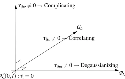
We thus identify four orthogonal directions for moving away from

N

(0,I): a move in the(la)

direction changes the mean and the variance of each coordinate while preserving Gaussianity and decorrelation; a move in the (lc) direction also preserves Gaussianity, doing so by introducing correlation between coordinates without changing their mean or their variances; a move in the(ha)

changes the marginal distributions (with constant means and variances) but preserves the mutual independence between coordinates; finally the direction(hc)corresponds to any change orthogonal to those previously listed, i.e. changes preserving both the marginal structure and the first and second order moment structure.

In our geometric picture, the distributions of interest are obtained as projections onto the prod-uct manifold

P

, onto the Gaussian manifold

G

, onto their span

P

∨

G

and onto their intersection

N

(0,I):η=0

G

L

P

L ηlc6=0→Correlating

ηha6=0→Degaussianizing ηhc6=0→Complicating

Figure 6: Three orthogonal directions away from

N

(0,I)in the local geometry. The origin

N

(0,I)

has coordinatesη= (ηla,ηlc,ηha,ηhc) = (0,0,0,0). For non-zero coordinates ηlc, the distribution labelled byηbecomes correlated while remaining Gaussian. Similarly, intro-ducing non-zero coordinatesηha de-Gaussianizes the marginal distributions, preserving the independence between components. Finally, introducing non-zero coordinatesηhc in-troduces a complicated dependency structure which is captured neither by the correlation structure nor by the marginals.

P(Y) ηla ηlc ηha ηhc

PP∨G(Y) ηla ηlc ηha 0

PG(Y) =

N

(EY,RY) ηla ηlc 0 0

PP(Y) =∏iPi(Yi) ηla 0 ηha 0

PP∧G(Y) =

N

(EY,diagRY) ηla 0 0 0

N

(0,I) 0 0 0 0

and is illustrated on Figure 6. In this figure, the “uninteresting direction”(la)which corresponds to location-scale changes is not displayed.

Divergences and objective functions. In accordance with decomposition (45), the small cumu-lant approximation Kφp,qof Equation (41) decomposes into four components:

K_φp,q=K_φlap,q+K_φlcp,q+K_φhap,q+K_φhcp,q (46)

where, for instance, K_φlap,qis the sum (41) with indices restricted to the set Ilaand similarly for the other terms. Now the divergence from P(Y)to its best uncorrelated Gaussian approximation

PP∧G(Y)reads

KP(Y),

N

(EY,diag(RY))

= KP(_Y˜_),

_N

_{(0,I) (47)}

≈ K_φP(_Y˜_),

N

_{(0,I) (48)}

= Dla(Y˜) +Dlc(Y˜) +Dha(Y˜) +Dhc(Y˜), (49)

is the cumulant-based approximation (29) to the KL divergence and where (49) defines the four components of this approximation, with the obvious notation

Dla(_Y˜_{) =K}la

φ P(Y˜),

N

(0,I), Dlc(Y˜) =KφlcP(Y˜),

N

(0,I),

and similarly for(ha)and(hc). Let us examine these components.

First, the entries of the standardized vector ˜Y have by construction the same mean and variance

as

N

(0,I). Therefore the distributions P(_Y˜_)and

_N

_{(0,I)have the same cumulants in the(la)set,} so that

Dla(_Y˜_{) =0.}

In the three other index sets (indexed by ha, lc, hc), the cumulants of

N

(0,I)cancel either because they are cross-cumulants of second order or because they are cumulants of order higher than 2. Thus, according to (41), these sums involve only the normalized cumulants ˜κ:

˜ κi1···ir

def

= cum(y˜1, . . . ,y˜r), (50)

arranged as

Dlc(_Y˜_{) =} 1

4_i

∑

_6=jκ˜ 2 i j,

Dha(_Y˜_{) =} 1

2_r

∑

_≥3 1

r!

∑

_i κ˜

2 i···i=

∑

i

Dha_i (_Y˜_{) where D}ha i (Y˜) =

1 2_r

∑

_≥3

1

r!κ˜

2 i···i,

Dhc(_Y˜_{) =} 1

2_r

∑

_≥3 1

r!_i

∑

1···ir6=

˜ κ2

i1···ir,

where∑i_1···ir6=denotes a sum over all r-uples in which the indices are not all identical.

We can now identify term-to-term the cumulant-based approximations with their exact Kullback-based expressions. Similarly to (29), we denote Iφ(Y), Gφ(Y),. . . , the expressions for I(Y), G(Y),. . . , obtained in the expansion aroundφand we have

C(Y) ≈ Cφ(Y) =Dlc(_Y˜_),

I(Y) ≈ Iφ(Y) =Dc(Y˜) =Dlc(Y˜) +Dhc(Y˜) =Cφ(Y) +Dhc(Y˜),

G(Y) ≈ Gφ(Y) =Dh(_Y˜_{) =D}ha_{(Y˜) +D}hc_{(Y˜) =∑iG}

φ(Yi) +Dhc(Y˜),

G(Yi) ≈ Gφ(Yi) =Dhai (Y˜),

which can be summarized as

Iφ(Y) =Dc(_Y˜_{) ∑iGφ(Yi)}

z }| { z }| {

K_φP(Y),PP∧G(Y)= Dlc(_Y˜_{) + D}hc_{(Y˜) + D}ha_(Y˜)

| {z } | {z }

C_φ(Y) G_φ(Y) =Dh(_Y˜_{) .}

We recover the key property (16) in the form

I_φ(Y) +

∑

i

P(_Y˜₎

(0,ηlc,ηha,ηhc)

N

(E ˜Y,RY˜)

(0,ηlc,0,0)

PP∨G(_Y˜₎

(0,ηlc,ηha,0)

N

(E ˜Y,diag(RY˜))

(0,0,0,0)

∏iP(_Y˜_i)

(0,0,ηha,0)

P

L

G

L

Dhc(_Y˜₎

Dlc(_Y˜_{) D}lc_(Y˜)

Dha(_Y˜₎

Dha(_Y˜₎

Dc(_Y˜₎

Dh(_Y˜₎

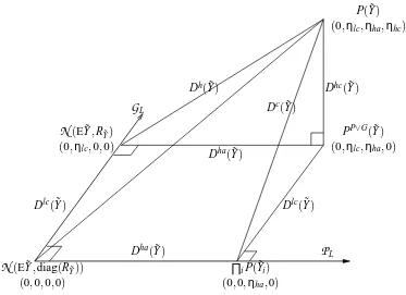
Figure 7: The local Euclidean geometry, tangent to the curved information geometry of Figure 4. The coordinates are the normalized cumulants of various types.

However, we now have an orthogonal decomposition in an Euclidean geometry:

Iφ(Y)−Cφ(Y) =Gφ(Y)−

∑

i

Gφ(Yi) =Dhc(Y˜)≥0. (52)

That is, for weakly correlated and weakly non-Gaussian vectors, dependence cannot be smaller than correlation and joint Gaussianity cannot be smaller than marginal Gaussianity, reaching the same conclusions as in Section 3.4. The “missing part” Dhc(_Y˜_)is

Dhc(_Y˜_{) =KφP,P}P∨G_≈KP,PP∨G_,

containing only high-order, cross-cumulants, i.e. it is due to the part of the log-density of Y which cannot be represented neither by linear-quadratic form in Y , neither by non-linear functions of Yi, nor by any linear combination of both kinds.

We note in the passing that Cφ(Y) =1₄∑i₆₌jκ˜2i j, which is identical to (15).

5. Conclusion

cumulants and Hermite polynomials which is derived via formal first- and second-order expansions. We have not tried to find conditions by which this derivation could be made rigorous but the results are perfectly in line with the insights gained at Section 3.4 and with common wisdom about ICA objectives.

A note on scaling. The entropy of a continuous variable (as opposed to a discrete variable) cannot be directly related to the notion of information because it is not invariant under invertible transforms. To give it some meaning, one must introduce some extraneous quantity like an hypothetical “reso-lution” or the “level” of some additive Gaussian noise. Such a trick is needed to apply the infomax principle to ICA, as done by Bell and Sejnowski (1995), or to relate non Gaussianity to entropy. Thus, using differential entropy in a noise-free context should always be taken with a grain of salt. In contrast, quantities like I(Y), C(Y), G(Y), defined in terms of the Kullback-Leibler divergence which itself is defined independently of a reference scale or of a reference measure. We note, in particular that the whole picture of Figure 2 is invariant with respect to the rescaling of any entry of Y .

Joint and marginal structures. This paper has described the interplay between dependence, cor-relation and Gaussianity, in particular in the ICA framework (17). Expression (17) shows a striking feature: on one hand, the dependence I(Y)is a property of the joint distribution of Y ; on the other hand, Equation (17) offers a decomposition of the dependence such that all the joint structure is captured in the correlation C(Y)with a remaining term (the marginal Gaussianities) depending only on the marginals of the distribution. It thus seems that all the dependencies between the entries of Y are captured by C(Y) which, however, is only a measure of second order independence. An explanation of this apparent paradox is that the constant term in (17), equal to G(Y), is constant

only under linear transforms of Y . It is only because ICA restricts itself to linear transforms that we

can forget about the dependencies which affect the value of G(Y) and which depend on the joint distribution of Y , indeed. It is fair to say that by restricting itself to linear transforms, ICA allows

the non-Gaussian part of the dependence to express itself only in the marginal distributions.

Other data models for ICA. An important application of ICA is to the blind separation of sources. This paper has focused onto the objective functions which arise in ICA theory when the sources are modeled as i.i.d. non-Gaussian processes. However, blind source separation can also be achieved by resorting to Gaussian models, providing some temporal (or spatial) structure of the source distributions can be exploited. Two popular approaches are to rely on the spectral diversity of stationary sources or on time diversity of non-stationary sources. Within these two kinds of model, the information-geometric view is strikingly similar. In particular, similar to the key relation (17), mutual information appears as the correlation minus the sum of marginal “non-properties:” diver-gence from spectral whiteness or from stationarity of the source processes (see Cardoso, 2001).

Acknowledgments

Appendix A. Orthogonality Between the Gaussian and the Product Manifold

We explain in which sense the Gaussian manifold

G

and the product manifold

P

intersect orthog-onally. Two smooth manifolds intersect orthogonally at a given point if their tangent planes at this point are orthogonal. Thus, to discuss the orthogonality between

P

and

G

at a point

N

(µ,R)where

R is diagonal, we must introduce the notion of tangent planes and of orthogonality between vectors

of tangent planes. This appendix is only intended for the curious reader (but see also Section 4 for using the notion of tangent plane) and is not necessary for understanding the rest of the paper; it is also both technical and lacking in rigor. For a mathematical treatment of tangent planes in non-parametric models, see e.g., Bickel, Klaassen, Ritov, and Wellner (1993).

We do not need to discuss tangent planes to manifolds in full generality because, in information geometry, tangent planes have a special representation: the vectors of a tangent plane are zero-mean random variables and orthogonality between two “vectors” is the decorrelation between the two associated random variables. This process is now described, starting with the easy case of finite-dimensional families of distributions and then showing how it may be extended to non-parametric families.

Let P be a point in

M

a L-dimensional statistical manifold, that is, distribution p(y) =p(y;θ?)

for some valueθ? ofθwhich is a vector of L real parameters. The tangent space of

M

at P is the linear space

( _L

∑

i=1

aili(y)

)

with li(y) =

∂log p(y;θ)

∂θi

_θ=θ? (53)

where each aiis an arbitrary coefficient. Thus, the score functions li(y)form a basis of the tangent plane and the ai are the coordinates of a vector of the tangent plane on this basis. In the tangent plane, the metric is given by the Fisher information matrix: if two vectors have coordinates {ai} and{bi}, their scalar product is ∑i jFi jaibj where Fi j =E(li(y)lj(y)). It follows that if f(y) and

g(y)are two vectors of the tangent plane, their scalar product simply is E(f(y)g(y)); in particular, orthogonality means decorrelation.

Similarly, we can obtain tangent vectors without resorting explicitly to parameters by noting that, if Q is close to P in

M

, it has parametersθ=θ?+δθwhereδθis a small vector ofRLso that, at first order,

L

∑

i=1

δθili(y) = L

∑

i=1

∂log p(y;θ?)

∂θi (θi−θ?i)≈log

p(y;θ) p(y;θ?) =log

q(y) p(y) ≈

q(y)−p(y)

p(y) .

This is the key for understanding how a non-parametric model is mapped locally to a linear space: a distribution Q infinitesimally close to P is mapped to the random variableε(y) = (q(y)−p(y))/p(y)

which has zero-mean under P and infinitesimally small variance. The tangent plane is the linear spaced spanned by these random variables. Conversely, an infinitesimal random variableε(y)with zero-mean under P is a vector by which P is shifted to Q, infinitesimally close to P, with density

q(y) =p(y)(1+ε(y)).