Learning Translation Invariant Kernels for Classification
Kamaledin Ghiasi-Shirazi [email protected]
Reza Safabakhsh [email protected]
Computer Engineering Department Amirkabir University of Technology Tehran, 15914, Iran
Mostafa Shamsi M [email protected]
Faculty of Mathematics and Computer Science Amirkabir University of Technology
Tehran, 15914, Iran
Editor: John Shawe-Taylor
Abstract
Appropriate selection of the kernel function, which implicitly defines the feature space of an algo-rithm, has a crucial role in the success of kernel methods. In this paper, we consider the problem of optimizing a kernel function over the class of translation invariant kernels for the task of binary classification. The learning capacity of this class is invariant with respect to rotation and scaling of the features and it encompasses the set of radial kernels. We show that how translation invariant kernel functions can be embedded in a nested set of sub-classes and consider the kernel learning problem over one of these sub-classes. This allows the choice of an appropriate sub-class based on the problem at hand. We use the criterion proposed by Lanckriet et al. (2004) to obtain a func-tional formulation for the problem. It will be proven that the optimal kernel is a finite mixture of cosine functions. The kernel learning problem is then formulated as a semi-infinite programming (SIP) problem which is solved by a sequence of quadratically constrained quadratic programming (QCQP) sub-problems. Using the fact that the cosine kernel is of rank two, we propose a formula-tion of a QCQP sub-problem which does not require the kernel matrices to be loaded into memory, making the method applicable to large-scale problems. We also address the issue of including other classes of kernels, such as individual kernels and isotropic Gaussian kernels, in the learning process. Another interesting feature of the proposed method is that the optimal classifier has an expansion in terms of the number of cosine kernels, instead of support vectors, leading to a remark-able speedup at run-time. As a by-product, we also generalize the kernel trick to complex-valued kernel functions. Our experiments on artificial and real-world benchmark data sets, including the USPS and the MNIST digit recognition data sets, show the usefulness of the proposed method.
Keywords: kernel learning, translation invariant kernels, capacity control, support vector ma-chines, classification, semi-infinite programming
1. Introduction
success of kernel methods. In fact, as shown by Xiong et al. (2005), if the kernel function is not chosen appropriately, it may even worsen the performance of an algorithm. This significant impact on the performance of the kernel-based algorithms and the fact that the appropriate feature space is problem-dependent, have driven researchers to devise various algorithms to learn the kernel function from the problem data.
The earliest method for learning a kernel function is cross-validation which is very slow and is only applicable to kernels with a small number of parameters. Cristianini et al. (1998) proposed an algorithm for adapting kernel functions with only one unconstrained parameter. Instead of optimiz-ing the parameters of a kernel, Amari and Wu (1999) suggested conformal transformation of the kernel function and proposed an algorithm for learning the parameters of the new kernel. Chapelle et al. (2002) devised a gradient-based algorithm for local optimization of a kernel with multiple un-constrained parameters. Glasmachers and Igel (2005) proposed a gradient-based method for learn-ing the covariance matrix of Gaussian kernels (Note that since the covariance matrix of a Gaussian kernel is constrained to be positive semi-definite, the method of Chapelle et al. (2002) cannot be used for learning this matrix). Ong et al. (2005) introduced the notion of hyperkernels and used it for kernel learning. They formulated the kernel learning problem as a functional with three terms: an empirical quality functional, a regularization term that penalizes the functions in a reproducing kernel Hilbert space (RKHS), and another regularization term that penalizes the kernels in a hyper reproducing kernel Hilbert space.
A milestone in the kernel learning literature is the introduction of the multiple kernel learning (MKL) framework by Lanckriet et al. (2004). They considered the problem of finding the optimal convex combination of multiple kernels and formulated it as a quadratically constrained quadratic programming (QCQP) problem. They also introduced a generalized performance measure which encompasses the hard-margin, 1-norm soft-margin, and 2-norm soft-margin performance measures as special cases. Although these performance measures have extensively been used for learning the optimal separating hyperplane in SVMs, their use as performance measures for kernel selection was unprecedented. Since the formulation of the resulting QCQP requires storing several kernel matrices in memory, their method was only applicable to problems with a small number of training samples. Bach et al. (2004) introduced an SMO-based algorithm to widen the range of solvable MKL problems by using the Moreau-Yosida regularization technique. Sonnenburg et al. (2005, 2006) reformulated the MKL problem as a semi-infinite linear program (SILP) which was then re-duced to training a sequence of classical SVMs with a single kernel for which several sophisticated large-scale algorithms exist. Rakotomamonjy et al. (2008) argued that the main difficulty with the SILP formulation of Sonnenburg et al. (2006) is that its objective function is non-smooth and intro-duced an equivalent convex formulation with a smooth objective function. Using convexity of the problem and the smoothness of the objective function, they proposed a reduced gradient algorithm for MKL which is also applicable to large-scale problems. The weakness of the reduced gradient algorithm is that, in contrast to to the SILP algorithm, it does not use the information collected in the previous points in the calculation of the next point. Combining the strengths of the SILP method of Sonnenburg et al. (2006) with those of the reduced gradient method of Rakotomamonjy et al. (2008), Xu et al. (2008) proposed an extended level method which is remarkably faster than both methods.
result proved by Schoenberg (1938) which states that every continuous radial kernel belongs to the convex hull of radial Gaussian kernels. They also proposed an efficient DC programming algorithm for numerically learning radial kernels in Argyriou et al. (2006). Gehler and Nowozin (2008) refor-mulated the optimization problem of Argyriou et al. (2006) as a semi-infinite programming problem and proposed the IKL (infinite kernel learning) framework for solving it numerically.
In this work, we consider the class of translation invariant kernel functions which encompasses the class of radial kernels as well as the class of anisotropic Gaussian kernel functions. This class contains exactly those kernels which can be defined solely based on the difference of kernel argu-ments; that is, the kernel functions with the property:
k(x,z) =˜k(x−z).
The general form of continuous translation invariant kernels onRnwas discovered by Bochner (1933). He proved that every function of the form1
k(x,z) =˜k(x−z) =
Z
Rne
jγT(x−z)dV(γ) (1)
is positive semi-definite, where V(.) is a monotonically increasing bounded function and the integra-tion is in the Lebesgue-Stieltjes sense. He also proved that, conversely, every continuous translaintegra-tion invariant positive semi-definite kernel function can be represented in the above form. In statistics, the translation invariance property is referred to as the stationarity of the kernel function. Genton (2001) and Sch¨olkopf and Smola (2002) give a list of the properties of this class along with impor-tant examples of stationary kernel functions, including the Gaussian, exponential, rational quadratic, and Bnspline kernels.
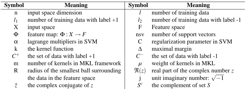
The rest of the paper proceeds as follows: Table 1 lists the choice of notations for familiar concepts in the field. Notations specific to this paper will be introduced in the course of discussions. Although the kernel learning formulation of Micchelli and Pontil (2005) contains a regularization term for controlling the complexity of the RKHS associated with the kernel function, there is no mechanism for controlling the capacity of the class of admissible kernels. In our formulation, we have provisioned a mechanism for controlling the complexity of the class of admissible kernels which is described in Section 2. The idea is to multiply a vanishing function inside the integral of Equation (1). In addition to controlling the capacity of the learning machine, this choice substitutes the compactness assumption of the integration region made by Micchelli and Pontil (2005). In Section 3, we propose a learning criterion which is essentially a reformulation of the generalized performance measure of Lanckriet et al. (2004). The proposed criterion ensures the compactness of the parameter space of SVM, and gives a probabilistic meaning to the regularization parameter of the 2-norm soft-margin SVM. The problem of finding an optimal kernel which minimizes this criterion over the class of translation invariant kernels leads to (4) which is our main variational problem.
In Section 4, we prove some important theorems which pave the way for an algorithmic solution to this problem. First, in Section 4.1 we prove the existence of an optimal solution for problem (4).
1. In this paper we will represent translation invariant kernels both as k :Rd×Rd →Cwith two arguments and as
In Section 4.2, we prove that the min and max operations in (4) can be interchanged, provided that the integration region is replaced by a compact set. In addition, it will be shown that the optimal kernel is a finite mixture of the basic kernels of the form kγ(x,z) =exp(jγT(x−z)). In Section 4.3, it will be proved that the integration region can indeed be replaced by a compact set. To solve problem (4) numerically, we introduce a semi-infinite programming (SIP) formulation in Section 4.4. In Section 4.5, using a topological argument, the issue of including other classes of kernels in the learning process will be addressed. It is well known that the regularization parameter of the 2-norm SVM, usually denoted byτ, can be regarded as the weight of a Kronecker delta kernel function, which is incidently a translation invariant kernel, as well. In Section 4.4 we introduce the semi-infinite programming problem (19) which is our main numerical optimization problem and corresponds to the simultaneous learning of the optimal translation invariant kernel as well as the parameterτ. As another application of the discussion of Section 4.5, in Section 4.7 we will introduce a method for learning the best combination of stabilized translation invariant kernels and isotropic Gaussian kernels.
In Section 5, we address the problem of numerically solving (19) on a computer. The proposed optimization algorithm is a variant of the class of local-reduction-based algorithms for solving SIP problems. An important feature of the proposed optimization algorithm is that it does not require loading the kernel matrices into memory and so it is applicable to large-scale problems. As stated above, it will be shown in Section 4.2 that the optimal kernel is complex-valued. Since algorithms are usually designed for real Euclidean spaces, this complicates the application of the kernel trick to the optimal kernel (consider for example an algorithm that checks the sign of a dot product). In Section 6, we show that the feature space induced by the real part of a complex-valued kernel is essentially equivalent to the original complex-valued kernel and deduce that the optimal real-valued kernel is a mixture of cosines. Yet another astounding feature of the proposed method is concerned with the evaluation time of the classifier which is even faster than a classical SVM with a single Gaussian kernel. Usually, multiple kernel learning methods yield a model whose evaluation time is in the order of the number of kernels times the number of support vectors. In Section 7, we show that the evaluation time of the optimal translation invariant kernel is proportional to the number of cosine kernels, regardless of the number of support vectors. In Section 8, using a learning theory discussion, we show the necessity of controlling the complexity of the class of translation invariant kernels.
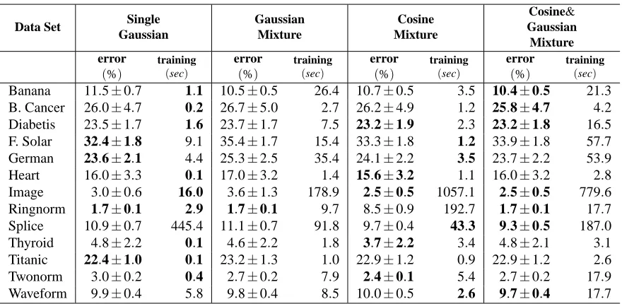
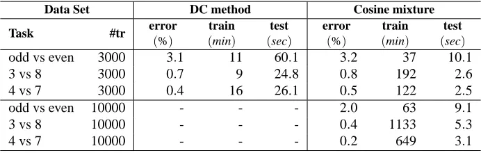
In Section 9, we will assess the practical usefulness of the proposed method on several data sets. In Section 9.1, we first perform some experiments on 13 artificial and real-world data sets collected from the UCI, DELVE, and STATLOG benchmark repositories by R¨atsch et al. (2001).In Section 9.2, we perform experiments on the USPS handwritten digit recognition data set, compar-ing the proposed method with the MKL of Chapelle et al. (2002). In Section 9.3, we compare the proposed method with the DC method of Argyriou et al. (2006) on the MNIST handwritten digit recognition data set. In Section 9.4, we experimentally assess the role of the capacity control mechanism of Section 2. Finally, we conclude the paper in Section 10.
2. A Hierarchy of Classes for Translation Invariant Kernels
Symbol Meaning Symbol Meaning
n input space dimension l number of training data
l1 number of training data with label +1 l2 number of training data with label -1
X input space F Feature space
Φ feature map:Φ: X→F nsv number of support vectors
α lagrange multipliers in SVM C regularization parameter in SVM
k the kernel function ∆ maximal margin
C+ the set of data with label +1 C− the set of data with label -1 m number of kernels in MKL framework µ weight of kernels in MKL R radius of the smallest ball surrounding ℜ(z) real part of the complex number z
the data in the feature space j unit imaginary number:√−1 ¯z the complex conjugate of z Sc the complement of set S
Table 1: Notations
that Equation (1) captures the general form of the large class of translation invariant kernels. To obtain the best tradeoff between approximation and estimation errors, we introduce a hierarchy of classes of translation invariant kernels. The appropriate class for a specific problem is then chosen by cross-validation. It must be mentioned that the idea of controlling the complexity of the class of admissible kernels has been previously used by Ong et al. (2005) for learning the kernels with hyperkernels. Although this type of complexity control is not provisioned by Micchelli and Pontil (2005), we, based on our experiments, believe that it is an important ingredient of the framework. To restrict the class of translation invariant kernels, we propose to limit the high frequency components of the kernel function. This is similar to the use of stabilizer functions in regularization theory (see Girosi et al., 1993). But, instead of adding a stabilizer function to the objective functional, which requires the determination of both the stabilizer and the regularization parameter, we explicitly define a nested class of translation invariant kernels
K
βas:K
β:=k(x,z) =
Z
Rne
jγT(x−z)G
β(kγk)d p(γ) : p is a probablity measure onRn
where β is defined on an ordered set, and Gβ:R+ →[0,1] is a decreasing continuous function with Gβ(0) =1 and Gβ(∞) =0. In addition, to ensure that these classes of kernels are nested, we require that Gβ1(r)≥Gβ2(r) for every r>0 and β1≤β2. Important candidates for Gβ(kγk) are
exp(−βkγk2)andkγk−βforβ>0. Note that we have left the choice of the norm to the application. Two important candidates are L1and L2norms. In Section 5, we will also assume that the function Gβ(kγk)is differentiable with respect toγ.
3. Kernel Selection Criterion
been studied and the authors suggested minimizing the radius-margin bound(R/∆)2as the preferred
criterion.
Consider the training set of a classification task consisting of the input-output pairs
{(x1,y1), ...,(xl,yl)}, with yi∈ {−1,1}. For a fixed kernel, support vector machines compute the maximal hard/soft margin separating hyperplane. By generalizing hard margin, 1-norm soft margin, and 2-norm soft-margin objective functions, Lanckriet et al. (2004) obtained the following general-ized criterion for 1/∆2(which must be minimized):
ω′
C′,τ′(k):= max
α: 0≤α≤C′,
αTy=0 (
2αTe−
l
∑
u=1l
∑
v=1αuαvyuyvk(xu,xv)−τ′αTα )
(2)
where e is the n×1 vector of ones and the prime sign is used to distinguish the parameters from those used in this paper. If (C′,τ′) is equal to (∞,0) ,(C′,0) , and (∞,1/C′), one obtains hard
margin, 1-norm soft margin, and 2-norm soft-margin performance measures, respectively. Our first change to this criterion is adding the constraint αTe=2. It has been shown (Crisp and Burges, 1999; Mavroforakis and Theodorodis, 2006) that by adjusting the parameters C and the offset b appropriately, this new constraint does not change the separating hyperplane. However, the new constraint plusαTy=0 gives∑i∈C−αi=∑i∈C+αi=1, which makes the exposition of our method
simpler. Furthermore, we divide (2) by 1+τ′ and define τ:= τ′
1+τ′. So, in this paper we use the criterion:
ωC,τ(k):=min
α∈A (
(1−τ)
l
∑
u=1l
∑
v=1αuαvyuyvk(xu,xv) +ταTα )
(3)
where
A
:=α∈Rl: 0≤α≤C,αTy=0,αTe=2 . Note that in the new criterion max{1
l1,
1
l2} ≤
C≤2 and 0≤τ≤1. This criterion works well for a fixed kernel by maximizing the margin∆. But in general, to minimize the radius-margin bound(R/∆)2, one must impose some constraint on the
radius R, as well. For translation invariant kernels we have R2=kΦ(x)k2=k(x,x) =˜k(0). Hence, bounding the radius R is equivalent to bounding ˜k(0). One can easily verify that bounding trace{K}, where K is the kernel matrix in the transductive framework (see Lanckriet et al., 2004, Equation 17), also leads to a bound on ˜k(0). Since by exploding R and trace{K}, the margin∆also explodes by the same amount, whilst the radius-margin bound remains constant, we from now on assume that ˜k(0) =1 and obtain the following optimization problem:2
sup k
min
α∈A (
(1−τ)
l
∑
u=1l
∑
v=1αuαvyuyvk(xu,xv) +ταTα )
s.t. k(x,z) =
Z
Rne
jγT(x−z)G
β(kγk)dV(γ)
Z
Rn dV(γ) =1,
V is monotonically increasing
or equivalently
sup p∈P(Rn)
min
α∈A Z
Rnα
TH(γ)αd p(γ) (4)
where
P
(Γ)denotes the set of all probability measures onΓand H(γ)is defined below. Let G(γ)be the l×l matrix whose(u,v)th entry is yuyvexp(jγT(xu−xv))Gβ(kγk). Define H(γ):= (1−τ)G(γ) + τIlwhere Ilis the l×l identity matrix. The following equation shows anO
(l)computational method for computingαTG(γ)α:αTG(γ)α= l
∑
u=1αuyuexp(jγTxu) 2 2
Gβ(kγk). (5)
4. Variational Optimization
In this section, we first prove the existence of a solution to problem (4). Next we prove that (4) can be written as a min-max problem with integration replaced by summation. This allows us to introduce a SIP formulation of the problem. We then introduce another SIP problem for learning the optimal kernel and parameterτ.
4.1 Replacing Sup with Max
We will prove that the sup operation in (4) can be substituted by the max operation. Note that all the variability in the choice of a probability measure p from
P
(Rn)collapses to the choice of an l×l matrixRRnH(γ)d p(γ)from S(Cl), where S(Cl)is the space of all l×l Hermitian complex-valued
matrices. So, it is sufficient to prove that the set of all these matrices is compact, which ensures that any sequence of these matrices has a convergent subsequence, and subsequently, the supremum value is achieved. Furthermore, by compacting the parameter space
A
in (3) there is no need to assume that the kernel matrices are strictly positive definite, as was done in Lemma 2 of Micchelli and Pontil (2005).Let C0(Rn)denote the function space of all continuous complex-valued functions defined onRn which vanish at infinity, that is, limkγk→∞g(γ) =0 for any g∈C0(Rn). By Theorem 3.17 of Rudin (1987), the function space C0(Rn)with the norm
kgk:=max
γ∈Rn|g(γ)|
is a Banach space. Note that the use of max operation is justified by the continuity and vanish-ing properties of g∈C0(Rn). Considering the above discussions, we need to prove the following theorem.
Theorem 1 For any fixed sample data Z={(x1,y1), ...,(xl,yl)}, the set
K
Z:= ZRnH(γ)d p(γ) : p∈
P
(Rn)
is a compact subset of S(Cl).3
Proof Consider any sequence(pn)in
P
(Rn). Define positive linear functionals Tn: C0(Rn)→C by Tng :=R
Rng(γ)d pn(γ). So, Tn∈C′0(Rn), the dual space of C0(Rn). Since for each n,kTnk=1,
by Banach-Alaoglu theorem (see for example Theorem 3.15 of Rudin, 1991 or page 237 of Royden, 1988), there exists some T ∈C′0(Rn) withkTk ≤1 and a subsequence(T
m)such that Tm→T in weak* topology. This means that for every g∈C0(Rn), we have Tmg→T g. Since, each element of the matrix H(γ)belongs to C0(Rn), it follows that
R
RnH(γ)dPm(γ)→T H. One can easily prove by contradiction thatkTk=1 and T is in fact a positive linear functional. By the Riesz representation theorem (see Theorem 6.19 of Rudin, 1987), the functional T can be represented uniquely by a complex Borel measure µ ,withR
Rnd|µ|=kTk=1, in the sense that
T g=
Z
Rng dµ for every g∈C0(
Rn).
The positivity of T implies that µ is a positive real measure. So,R
Rndµ=1 and consequently µ
is also a probability measure onRn. Thus,
Z
RnH(γ)d pm(γ)−→
Z
RnH(γ)dµ(γ)
which indicates that the set
K
Z is compact.4.2 Interchanging the min and max Operations
We first prove a theorem about interchanging the min and max operations which is an abstracted and generalized version of Theorem 20 in Micchelli and Pontil (2005).
Theorem 2 Assume thatΓis a compact Hausdorff space and the function g :Γ×Rl →Ris
con-tinuous in the first parameter and convex and differentiable in the second parameter. Let
E
andI
be finite index sets , ai, where i∈
E
∪I
, be l×1 vectors, and bi, where i∈E
∪I
, be real-valuedscalars. Considering problem (6), assume that the Slater’s condition (see Boyd and Vandenberghe, 2004) holds, that is, there exists someαsuch that aTi α=bifor all i∈
E
and aTi α<bifor all i∈I
.Then there exist a discrete probability measure ˜p∈
P
(Γ)with at most l+1 atoms and some feasiblepoint ˜αwhich solve the max-min problem
max
p∈P(Γ) α: aT min
iα=bifor i∈E, aT
i α≥bifor i∈I Z
Γg(γ,α)d p(γ) (6)
and the min-max problem
min
α: aTiα=bifor i∈E, aTi α≥bifor i∈I
max p∈P(Γ)
Z
Γg(γ,α)d p(γ) (7)
simultaneously. In addition, each atom of ˜p is a global maximum of g(γ,α˜)as a function ofγ.
3. Note that the topology of S(Cl)is the same as that ofRl2.An l×l hermitian matrix contains l real-valued diagonal
Proof Assume that ˆαand ˆp solve the problem (7). Define the function
φ:Rl→R φ(α):=maxγ∈Γ{g(γ,α)}
and the set
Γ∗:={γ:γ∈Γ,g(γ,αˆ) =φ(αˆ)}.
By Lemma 24 of Micchelli and Pontil (2005), the directional derivative ofφalong the direction
d∈Rl, denoted byφ′
+(α; d), is given by:
φ′
+(α; d) =maxγ ∈Γ∗
dT∇αg(γ,α) .
Since ˆαminimizes (7), we have
φ′
+(αˆ; d) =maxγ ∈Γ∗
dT∇αg(γ,α)|α=αˆ ≥0 (8)
for any direction d such that aTi d=0 for i∈
E
and aTi d≥0 for i∈I
∗, whereI
∗:={i∈I
: aT i α=bi}.
Let
M
be the convex hull of the set of vectorsN
:={∇αg(γ,α)|α=αˆ :γ∈Γ∗} ⊆Rl. SinceM
⊆Rl, by the Caratheodory theorem (see for example Section 17 of Rockafellar, 1970) every vector inM
can be expressed as a convex combination of at most l+1 elements ofN
. We claim that the setO
:= (∑
i∈E∪I∗λiai: λi≥0 for all i∈
I
∗ )intersects
M
. Assume, on the contrary, thatM
andO
are distinct. SinceM
is convex and compact andO
is convex and closed, by the strict separating hyperplane theorem (see corollary 11.4.2 of Rockafellar, 1970), there exists a separating hyperplane wTα+b=0, w∈Rl, b∈R, such that∑
i∈E∪I∗λiwTai+b>0, ∀λ: λi≥0 for i∈
I
∗and
wT∇αg(γ,α)|α=αˆ +b<0, ∀γ∈Γ∗. (9)
wTai=0, ∀i∈
E
,wTai≥0, ∀i∈
I
∗.By combining these results with (9), we get
max
γ∈Γ∗w T∇
αg(γ,αˆ)|α=αˆ <0.
This means that w is a feasible descent direction at ˆαwhich contradicts (8). So, the sets
O
andM
intersect. This means that there exist real numbers ˆλi, i∈E
, nonnegative numbers ˆλi, i∈I
∗,and a discrete probability measure ˆp with at most l+1 atoms such that
∑
i∈E∪I∗ˆ λiai=
Z
Γ∇αg(γ,αˆ)d ˆp. (10)
Now, we turn our attention to the solution of problem (6) for p=p. This is a convex opti-ˆ mization problem. Since by assumption the Slater’s condition holds, the KKT conditions provide a necessary and sufficient condition for optimality (see Boyd and Vandenberghe, 2004, page 244) and therefore a solution ˇαto problem (6) is found by solving the following KKT conditions:
∑
i∈E∪Iˇ λiai=
Z
Γ∇αg(γ,αˇ)d ˆp
aTi (αˇ) =0, i∈
E
aTi (αˇ)≥0, i∈
I
ˇλi≥0, i∈
I
ˇλi aTi αˇ−bi
=0, i∈
I
.By defining ˆλi=0 for i∈
I
\I
∗, using (10), and recalling the definition ofI
∗, it can be seen thatˆ
α,ˆλare the unique solution to the above KKT conditions. Thus, ˜α=αˆ and ˜p=p solve problemsˆ (6) and (7) simultaneously and the theorem follows.
Corollary 3 Assume that Γ is any compact subset of Rn and the parameter C is chosen4 such
that C>max{1
l1,
1
l2}. Then, there exist ˜α∈
Rn and ˜p∈
P
(Γ) that solve problems (11) and (12)simultaneously. Furthermore, ˜p is a discrete probability measure with at most l+1 atoms and each
atom of ˜p is a global maximum of ˜αTH(γ)α˜.
max p∈P(Γ)minα∈A
Z
Γα
TH(γ)αd p(γ), (11)
min
α∈Apmax∈P(Γ)
Z
Γα
TH(γ)αd p(γ). (12)
Proof It is sufficient to show that the Slater’s condition holds, that is, there existsα∈Rl such that αTe=2,αTy=0,α>0, andα<C. One can easily verify that the choiceαi= 1
l1 for i∈C
+and
αi= 1
l2 for i∈C
−satisfies these conditions.
In the rest of the paper, we assume that C>max{l1
1,
1
l2}.
4.3 Confining Integration to a Compact Region
To write (4) as a min-max optimization problem, we first proved in Section 4.1 that the sup operation can be replaced by the max operation. In the previous section we proved Corollary 3 which asserts that if the integration region of (4) could have been replaced by a compact set, then the max and min operations could also be interchanged. In this section, we show that the integration region of (4) can safely be confined to a compact subset ofRn. Let us first prove two useful lemmas.
Lemma 4 For arbitrary domains X and Y and every function f : X×Y →R, the following
inequal-ity holds:
sup x∈X
inf
y∈Yf(x,y)≤yinf∈Ysupx∈X f(x,y).
Proof Assume on the contrary that
sup x∈X
inf
y∈Yf(x,y)>yinf∈Ysupx∈X f(x,y).
Then, there exist ˜x∈X and ˜y∈Y such that
inf
y∈Y f(x˜,y)>supx∈X f(x,y)˜
which contradicts with the existence of f(x˜,y)˜ .
Lemma 5 Ifτ<1, then there exists some compact subsetΓβofRn, independent ofα, where allγ’s
that maximizeαTH(γ)αlie in it.5 Proof For eachα∈Rl we have
max
γ∈Rnα
TH(γ)α= (1
−τ)max
γ∈Rn
l
∑
u=1αuyuexp(jγTxu) 2 2
Gβ(kγk)
+ταTα. (13)
Let t(α)denote the maximum value of the term in the braces in the above equation. Since Gβ is continuous and Gβ(0) =1, there is an open ball around zero inRn such that G
β(kγk)>0. This fact plus the conditionαTe=2, ensure that the coefficient of at least one of the exponential terms in (13) is nonzero. Hence, the term in the braces in (13), as a function ofγ, is never identically zero and thus t(α)>0. For all values ofγwith Gβ(kγk)< t
αTH(γ)α−ταTα= l
∑
u=1αuyuexp(jγTxu) 2
Gβ(kγk)≤4Gβ(kγk)<t(α)
and the lemma’s assertion follows from limr→∞G(r) =0.
Theorem 6 There exists an optimal solution (α˜,p)˜ to problem (4) which is also a solution to it when the integration domain is confined to the compact setΓβ.
Proof Let(α˜,p)˜ be a solution to problems (6) and (7) withΓreplaced byΓβ. By Lemma 4 and Corollary 3, we have the following sequence of inequalities:
max p∈P(Γβ)minα∈A
Z
Γβ
αTH(γ)αd p(γ)≤
max p∈P(Rn)minα∈A
Z
Rnα
TH(γ)αd p(γ)
≤
min
α∈Ap∈maxP(Rn)
Z
Rnα
TH(γ)αd p(γ)
≤
min
α∈Ap∈maxP(Rn)
Z
Rnmaxγ∈Rnα
TH(γ)αd p(γ) =
min
α∈Amaxγ∈Rnα
TH(γ)α=
min
α∈Ap∈maxP(Γβ)
Z
Γβα
TH(γ)αd p(γ).
However, the first and the last terms are equal by Corollary 3.
4.4 Semi-infinite Programming Formulation
We have not yet addressed the problem of how (12) is to be really solved on a machine. In this section, we reformulate (12) as a semi-infinite programming problem for which many algorithms have been proposed (see Hettich and Kortanek, 1993; Reemtsen and G¨orner, 1998, for two reviews on the subject).
Theorem 7 Let ˜α and ˜t be a solution to the semi-infinite programming problem (14) and define the setΓHβ(α):=nγ∈Γβ:αTH(γ)α=maxγ∈ΓβαTH(γ)α
o
. Let (Q) be the QCQP problem that is
obtained by replacingΓβbyΓHβ(α˜)≡ {γ1, ...,γm}in (14) and let ˜µ1, ...,˜µmbe a set of Lagrange
mul-tipliers associated with the constraints t≥αTH(γi)α, 1≤i≤m which optimize the dual problem of (Q). If ˜p is the discrete probability measure defined by ˜p(γi):=µ˜i i=1, ...,m, then ˜αand ˜p solve
the problem (4). In addition, there exists a solution pair(α˜∗,p˜∗)such that ˜p∗contains at most l+1
minα,t t
s.t. t≥αTH(γ)α for all γ∈Γβ
0≤α≤C
αTy=0 αTe=2.
(14)
Proof Since for allγ∈/ΓH
β(α˜)the strict inequality ˜t>α˜TH(γ)α˜ holds, ˜αand ˜t also solve the
fol-lowing QCQP problem:
minα,t t
s.t. t≥αTH(γi)α i=1, ...,m
0≤α≤C
αTy=0 αTe=2.
In addition, from ˜t=α˜TH(γ
1)α˜ =...=α˜TH(γm)α˜, it follows that ˜αand ˜t also solve the
follow-ing problem:
min
α∈Aµ≥0,max∑m i=1µi=1
αT "
m
∑
i=1µiH(γi) #
α (15)
By Theorem 17 of Lanckriet et al. (2004), if ˜µ is chosen as specified by the statement of this theorem, then ˜αand ˜µ simultaneously solve the min-max problem (15) and the following max-min problem:
max µ≥0,∑m
i=1µi=1
min
α∈Aα T
" m
∑
i=1µiH(γi) #
α
which can also be written as
max p∈P(ΓH
β(α˜))
min
α∈A Z
αTH(γ)αdP(γ)
The first assertion of the theorem follows from the following inequalities:
˜t= max
p∈P(ΓH β(α˜))
min
α∈A Z
αTH(γ)αdP(γ)≤
max p∈P(Γβ)minα∈A
Z
αTH(γ)αdP(γ)
≤
min
α∈Ap∈maxP(Γβ)
Z
where the last equality follows from a simple reformulation of problem (14). The last part of the theorem follows from Corollary 3 and reversing the above proof.
4.5 Including Other Kernels in the Learning Process
Although the focus of this paper is on the task of learning translation invariant kernels, it is easy to furnish the set of admissible kernels with other kernel functions. For example, one may want to find the best convex combination of stabilized translation invariant kernels along with isotropic/non-isotropic Gaussian kernels, and polynomial kernels with degrees one to five.6 In general, assume that we have M classes of kernels
Ki:=
kγ(x,z): γ∈Γi i=1, ...,M
whereΓ1, ...,ΓMare distinct compact Hausdorff spaces. For i∈1, ...,M let Gi(γ)be the l×l matrix whose(u,v)’s entry is yuyvkγ(xu,xv)and define Hi(γ):= (1−τ)Gi(γ) +τIl. The problem of learning the best convex combination of kernels from these classes for classification with support vector machines can be stated as
sup p∈P(Γ0)
min
α∈A Z
Γ0
αTH
0(γ)αd p(γ) (16)
whereΓ0:=Γ1∪...∪ΓMand
H0(γ):=
H1(γ) i fγ∈Γ1 H2(γ) i fγ∈Γ2
.. .
HM(γ) i fγ∈ΓM .
The results of the previous sections will hold for this combined class of kernels if we prove that Γ0is a compact Hausdoff space and that h0(γ,α):=αTH0(γ)αis continuous with respect toγ. Let
T
idenote the topology onΓifor i∈1, ...,M. Define the setT
0of subsets ofΓ0as:T
0:={O1∪O2...∪OM: O1∈T
1,O2∈T
2, ...,OM∈T
M}. Proposition 8T
0is a topology.Proof ClearlyΓ0∈
T
0. Next we must show thatT
0is closed under arbitrary union. Let O=Si∈IOi where Oi∈T
0andIis an arbitrary index set. We haveO= [
j∈{1,...,M} [
i∈I Oi∩Γj
!
which shows that O∈
T
0. Finally, we should show that finite intersection of closed sets is a closed set. Assume that C=Tri=1Ci, where r∈Nand Cic∈
T
0. We haveCc= [
i∈{1,...,r}
Cic= [
i∈{1,...,r}
[
j∈{1,...,M}
(Cci ∩Γj).
Since CicandΓjare both open in
T
j, the set Cic∩Γjis open inT
j. By the properties of topologiesT
1, ...,T
Mand the definition of topologyT
0it follows that Cc∈T
0which shows that C is closed inT
0.Proposition 9 Assume that the functions hi(γ,α):Γi×Rl →R defined as hi(γ,α) =αTHi(γ)α,
where i=1, ...,M, are continuous in the first parameter. Then, the function h0(γ,α):Γ0×Rl →
R defined as h0(γ,α) =αTH(γ)α ,where the topology ofΓ
0 is
T
0, is also continuous in the first parameter.Proof Fixαto any value and define ¯hi(γ):=hi(γ,α)for i=0, ...,M. Let O be an open subset ofR. We must show that ¯h−01(O)is open in topology
T
0. We have¯h−1 0 (O) =
[
i=1,...,M ¯h−1
0 (O)∩Γi
= [ i=1,..,M
¯h−1
i (O).
Since the set ¯h−i 1(O)is open in
T
i for each i∈ {1, ...,M}, it follows from the definition ofT
0 that the union of these sets is also open inT
0. So, ¯h−01(O)is open inT
0and the result follows. Proposition 10 The setΓ0with topologyT
0is compact in itself.Proof Let O={Oi: i∈
I
0} be an open covering of Γ0, whereI
0 is some index set. Let j beany number in the set{1, ...,M}. SinceΓj ⊆Γ0, the set O is also an open covering forΓj. By compactness ofΓj, there exists a finite index set
I
j⊆I
0 such that the set
Oi: i∈
I
j is an open subcovering ofΓj. Thus, the set{Oi: i∈I
1∪...∪I
M} is a finite open subcovering ofT
0 whichproves thatΓ0is compact.
Proposition 11 Assume that topologies
T
1, ...,T
Mare Hausdorff. Then, so is the topologyT
0. Proof We must prove that for any two pointsγ1,γ2∈Γ0there are disjoint open sets O1and O2suchthatγ1∈O1 and γ2∈O2. If γ1 andγ2 belong to the same set Γj for some j∈1, ...,M, then the assertion follows from the Hausdorffness property of
T
j. Without loss of generality, assume that γ1∈Γ1andγ2∈Γ2. The choice O1=Γ1and O2=Γ2completes the proof.Theorem 12 Assume that Γ1, ...,ΓM are compact Hausdorff spaces and the matrices Hj are as
defined previously in this section. Furthermore, assume that for j=1, ...,M the functions hj(γ,α): Γj→Rl defined by hj(γ,α):=αTHj(γ)α are continuous in the first parameter. Let ˜αand ˜t be a
minα,t t
s.t. t≥αTH1(γ)α for all γ∈Γ1 ..
.
P(Γ1, ...,ΓM):= t≥αTHM(γ)α for all γ∈ΓM (17)
0≤α≤C
αTy=0 αTe=2.
Define the setΓHj(α):=γ
∈Γj:αTHj(γ)α=maxγ∈ΓjαTHj(γ)α . Let (Q) be the QCQP
prob-lem that is obtained by replacing everyΓj with j=1, ...,M byΓHj (α˜)≡ n
γj
1, ...,γ
j mj
o
in (17). For
any j∈ {1, ...,M}let ˜µ1j, ...,˜µmjj be a set of Lagrange multipliers associated with the constraints t≥αTHj(γij)α, 1≤i≤mj which optimize the dual problem of (Q). If ˜p is the discrete probability
measure defined by ˜p(γij):=˜µij i=1, ...,mj j=1, ...,M, then the pair(α˜,p)˜ solves the problem
(16). In addition, there exists a solution pair(α˜∗,p˜∗)such that ˜p∗ contains at most l+1 nonzero
atoms.
Proof The result is immediately obtained by replacing the setΓβbyΓ0in Theorem 7. 4.6 Automatic Adjustment of the Parameterτ
In this section, we consider the following problem:
max
0≤τ≤1,p∈P(Rn)minα∈A Z
Rnα
TH(γ)αdP(γ). (18)
It is well known that the parameterτcan be envisioned as the weight of the kernelδ(x,z), where δ is the Kronecker delta function. So, the problem of learning the parameter τ is equivalent to choosing the best convex combination of the set of translation invariant kernels augmented with the delta kernelδ(x,z). By using Theorem 12 we get the following corollary.
Corollary 13 Let ˜αand ˜t be a solution to the semi-infinite programming problem Pτ(Γβ), where for each compact setΓthe problem Pτ(Γ)is defined by (19). Define the set
ΓG β(α):=
n
γ∈Γβ:αTG(γ)α=maxγ∈ΓβαTG(γ)αo.
Let (Q) be the QCQP problem that is obtained by replacingΓbyΓGβ(α˜)≡ {γ1, ...,γm}in (19) and let
˜µ1, ...,˜µmbe a set of Lagrange multipliers associated with the constraints t≥αTG(γi)α, 1≤i≤m
which optimize the dual problem of (Q). In addition, let ˜µ0be a Lagrange multiplier associated with the constraint t≥αTαin the dual problem of (Q). If ˜p is the discrete probability measure defined
by ˜p(γi):=˜µi i=1, ...,m and ˜τ:=˜µ0, then ˜α, ˜τ, and ˜p solve the problem (18). In addition, there
Pτ(Γ):=
minα,t t
s.t. t≥αTG(γ)α for all γ∈Γ t≥αTα
0≤α≤C
αTy=0 αTe=2.
(19)
Proof Letω0∈/Γβand assign the kernelδ(x,z)to this point. The corollary is proved by applying
theorem 12 to the setsΓβand{ω0}.
4.7 Furnishing the Class of Admissible Kernels with Isotropic Gaussian Kernels
Although the class of translation invariant kernels encompasses the class of Gaussian kernels with arbitrary covariance matrices, the stabilized class of translation invariant kernels
K
βdoes not. So, it may be advantageous to combine the classK
βwith the class of Gaussian kernels. In this section, we consider learning the best convex combination of kernels of the classesK
βand the stabilized class of isotropic Gaussian kernelsK
η:=k(x,z) =
Z
R
e−ωkxu−xvk2e−ηkωk2d p(ω) : p is a probablity measure onR
whereη>0. We also learn the parameterτautomatically. The proof that there exists some compact setΩη⊆R where we can confine the integration to it parallels the discussion of Section 4.3 and is
omitted. By using Theorem 12, it follows that the expansion of the optimal kernel along with the weight of each kernel can be obtained by solving the SIP problem Pτ(Γβ,Ωη), where Pτ(Γ,Ω) is defined as:
Pτ(Γ,Ω):=
minα,t t
s.t. t≥αTG(γ)α for all γ∈Γ
t≥
l
∑
u=1l
∑
v=1αuαvyuyve−ωkx−zk
2
e−ηkωk2 for all ω∈Ω
t≥αTα
0≤α≤C
αTy=0 αTe=2.
5. Optimization Algorithm
We now turn to the problem of numerically solving the nonlinear convex semi-infinite programming problem Pτ(Γβ).7 The term semi-infinite stems from the fact that whilst the number of variables is
finite, there is an infinite number of constraints which are indexed by the compact setΓβ. Hopefully, for each finite setΓ⊆Γβ, the problem Pτ(Γ)is QCQP and therefore convex. Hence, in principle, one can construct a sequence of QCQP problems with an increasing number of constraints such that their solutions converge to the solution of problem Pτ(Γβ). This is the principle used by discretization and exchange algorithms (see Hettich and Kortanek, 1993; Reemtsen and G¨orner, 1998). On the other hand, by Corollary 13, only a finite number of constraints will be active in a solution. Furthermore, it is easy to show that this property is not limited to a solution point, and the active constraints at a solution also identify the active constraints in a neighborhood of it. This is the principle behind the methods based on local reduction (see Reemtsen and G¨orner, 1998; Hettich and Kortanek, 1993). Reemtsen and G¨orner (1998) proposed that to further speed up the methods based on local reduction, the set of active constraints be locally adapted. Combining these ideas with numerous experiments, we arrived at Algorithm 1. This algorithm is very similar to Algorithm 7 in Reemtsen and G¨orner (1998) which is based on local reduction.
5.1 Choosing the Initial Value ofα
We choose the initial value ofαsuch that maximizing the criterion (3) with respect to the kernel function k and the parameter τ correspond to maximizing the distance of the means of the two classes in a feature space. Let us first write the distance between means of two classes in the feature space of some kernel k′
km1−m2k2=
1
l1u
∑
∈C+Φ(xu)− 1
l2v
∑
∈C− Φ(xv)2
= 1
l12u∈
∑
C+v∑
∈C−k′(xu,xv) +2 1
l1l2u∈
∑
C+v∑
∈C−k′(xu,xv) + 1
l22u
∑
∈C−v∈∑
C−k′(xu,xv).
By choosingαi=1/l1for i∈C+andαi=1/l2for i∈C−, we have
km1−m2k2=
l
∑
u=1l
∑
v=1αuαvyuyvk′(xu,xv).
Comparing the above equation with (3), we see that maximizing the criterion (3) with respect to the kernel function k and the parameterτis equivalent to maximizing the distance between means of the samples of the two classes in the feature space of kernel k′(x,z) =k(x,z) +τδ(x,z). Note that this choice forαalso satisfies the required conditionsαTe=2,αTy=0, and max{l1
1,
1
l2} ≤α≤C;
and thusα∈
A
.5.2 Global Search for Local Maxima ofαTG(γ)α
values ofγwhich locally maximize the functionαTG(γ)αfor givenα. Here we also assume that the function Gβ(kγk)is differentiable with respect toγ. The choice of limited-memory BFGS algorithm (Nocedal, 1980; Liu and Nocedal, 1989; Nocedal and Wright, 2006) for this optimization is very important. For large-scale problems with large n, the memory needed to store the Hessian matrix and the associated computations become prohibitive. Although a gradient-ascent algorithm does not compute the Hessian matrix, its convergence rate is very slow. The limited-memory BFGS algorithm provides an excellent practical compromise between the computations at each step and the number of iterations till convergence, without storing the full Hessian matrix in memory.
Algorithm 1 General Optimization Algorithm Require: T1
1. Γ(0)← {} , t(0)← l1
1+
1
l2
{A lower bound for parameter t is the minimum value ofαTαforα∈
A
}2. Initializeα(0)as described in Section 5.1
3. for i=1,2, ...do
4. set R such that for allγwithkγk>R, the relationαTG(γ)α<t(i−1)holds for allα
5. Γ(gi)←GlobalSearchForLocals(α(i−1),R)
{denote the maximum value obtained by the global search by s(i)}
6. Γ(si)←Γ(i−1)SΓ(gi)
7. Solve problem Pτ(Γ(si))to obtain the optimal parameters ts(i),α(si)and µ(si)
{see Section 5.3}
8. Locally adaptΓ(si)and µs(i)to obtain the optimal parameters tl(i),α(li),Γ(li)and µ(li)
{see Section 5.4}
9. t(i)←tl(i),α(i)←α(li)
10. Construct µ(i)andΓ(i)by eliminating zero indices of µ(li)along with the corresponding vectors inΓ(li)
11. if t(i)−t(i−1)<εt(i−1)or i=T1then
12. terminate algorithm with the kernel k(x,z):=∑m j=1µ
(i)
j cos
(x−z)Tγ(i) j
{we assume thatΓ(i)=nγ1(i), ...,γ(mi) o
and that µ(ji) is the Lagrange multiplier associated
with the constraintαTG(γ(ji))α≤t in problem Pτ(Γ(i))} 13. end if
14. end for
5.3 Solving the Problem Pτ(Γ)for Finite SetΓ
LetΓ={γ1, ...,γm}be a finite subset ofΓβ. Since Γis finite, the problem Pτ(Γ)can be written as
Algorithm 2 GlobalSearchForLocals Require: α, R, T2, and T3
1. Γ={},i=0
2. for j=1,2, ...do
3. generate a random point x∈Rn
4. generate a random number r∈[0,R] 5. γ0←rkxxk
6. starting from γ0 and using the limited-memory BFGS algorithm find a local maximum γ(i)
for functionαTG(γ)α 7. ifγ(i)∈Γthen
8. i←i+1{count the number of repeating local maxima} 9. end if
10. Γ←Γ∪γ(i)
11. if(i− |Γ|)≥T2or j=T3then
12. return Γ
13. end if 14. end for
minα,t t
s.t. t≥αTG(γi)α for all i=1, ...,m t≥αTα
0≤α≤C
αTy=0 αTe=2.
(20)
This problem has been studied in Section 4.6 of Lanckriet et al. (2004) and it has been suggested to store the l×l kernel matrices G(γ1), ...,G(γm) in memory and solve the problem with general purpose software packages. But, the memory requirement of this approach limits its applicability to small-sized problems. However, the facts that
αTℑ
{G(γ)}α=0
and
ℜ{G(γ)}=vc(γ)Tvc(γ) +vs(γ)Tvs(γ),
vc(γ):=
y1cos(γTx1), y2cos(γTx2), . . . ,ylcos(γTxl)
, vs(γ):=
where ℜ{z} and ℑ{z} are the real and imaginary parts of z, respectively, show that the kernel matrices G(γ1), ...,G(γm)appearing in problem (20) are effectively8of rank two. This allows us to reformulate (20) as a new QCQP problem as follows:
minα,t,c,s t
s.t. t≥c2i +s2i i=1, ...,m ci=
l
∑
u=1αiyicos(γTi xu) i=1, ...,m
si= l
∑
u=1αiyisin(γTi xu) i=1, ...,m
t≥αTα
0≤α≤C
αTy=0 αTe=2.
(21)
Now, there is no need to load the kernel matrices into memory and so general-purpose QCQP solvers such as Mosek (Andersen and Andersen, 2000) can be used to solve (21) even when the training set size is huge.
5.4 Local Adaptation
As stated in the previous section, for any finite setΓ={γ1, ...,γm} ⊆Γβ, the problem Pτ(Γ)is convex
and so every local solution is also globally optimal. But, if we consider the valuesγ1, ...,γmas points
in the spaceRn, we get the following non-convex optimization problem:
max µ≥0,µTe=1,
γ1, ...,γm∈Rn min
α∈A m
∑
i=1µiαTG(γi)α+µ0αTα. (22)
Now, we can use the the solution of the problem Pτ(Γ)obtained in the previous section as the starting point for problem (22) and locally improve it by an ascent method. By unrolling (22), we obtain the following optimization problem:
max µ∈Rm+1,
γ1, ...,γm∈Rn ˆ
J(µ,γ1, ...,γm) s.t. µ≥0,µTe=1 (23)
where
ˆ
J(µ,γ1, ...,γm):=
min
α∈A (
l
∑
u=1l
∑
v=1αuαvyuyv m
∑
i=1µiGβ(kγik)cos(γTi (xu−xv)) +µ0
l
∑
u=1α2
u )
. (24)
Problem (23), corresponds to adapting the kernel parametersγ1, ...,γmand µ0, ...,µmof the kernel function k(x,z) =∑m
i=1µicos(γTi (x−z)) +µ0δ(x−z) for the task of SVM classification, where δ denotes the Kronecker delta function. This problem has been previously studied by Chapelle et al. (2002) for general kernel functions with unconstrained parameters and they proved that the function
ˆ
J(.)is differentiable provided that problem (24) has a unique solution.9 They also proposed a simple gradient-based iterative algorithm for adapting the kernel parameters. Recently, Rakotomamonjy et al. (2008) performed a more detailed analysis of this problem in MKL and proposed a reduced gradient algorithm with line search. They reasoned that since the computation of the function ˆJ is
costly,10the overhead of a line search preserves the effort.
To avoid the difficulties of the constrained optimization, we replace the constrained vector µ by the unconstrained vectorρ, connected by the relation µi= ρ
2
i
ρTρ, i=0, ...m, and rewrite (23) as the
following problem:
max
ρ∈Rm+1,
γ1, ...,γm∈Rn
J(ρ,γ1, ...,γm) (25)
where
J(ρ,γ1, ...,γm):=
min
α∈A 1 ρTρ
( l
∑
u=1l
∑
v=1αuαvyuyv m
∑
i=1ρ2
iGβ(kγik)cos(γTi (xu−xv)) +ρ20
l
∑
u=1α2
u )
. (26)
We use the limited-memory BFGS algorithm to numerically solve (25). Our experiments on MKL tasks show that the method proposed in this section is several times fatser than the reduced gradient algorithm of Rakotomamonjy et al. (2008).11 It has been also stated by Rakotomamonjy
et al. (2008) that their method could be improved if the Hessian matrix could be computed ef-ficiently. This is not the case for the problem (25) with m×(n+1) variables; where, even for moderate size problems, the storage of the Hessian matrix requires lots of memory.
5.5 Solving the Intermediate SVM Problem and Its Gradient
To compute the function J(.)defined by Equation (26), we have to solve the following constrained quadratic programming problem:
9. Truely speaking, the proof should be credited to Danskin (1966).
10. Although the definition of the function J in Rakotomamonjy et al. (2008) differs from (24), computation of both functions corresponds to training a single-kernel SVM.
minα αT m
∑
i=1ρ2
i ρTρG(γi)
! α+ ρ
2 0
ρTρα Tα
s.t. 0≤α≤C
αTy=0 αTe=2.
(27)
Although the traditional algorithms for solving quadratic programming problems, such as active set methods, are fast, they need to store the kernel matrix in memory which prevents their application in large-scale problems. So, various algorithms for large-scale training of SVMs, such as SMO (Platt, 1999) or SV MLight (Joachims, 1999), have been proposed. Again, since the effective rank of the kernels G(γ1), ...,G(γm)is two, we can re-state the problem (27) in a memory efficient manner
as:
minα,c,s ρ2
0
ρTρα
Tα+
∑
m i=1ρ2
i ρTρ c
2
i +s2i
s.t. ci= l
∑
u=1αuyucos(γTi xu) i=1, ...,m
si= l
∑
u=1αuyusin(γTi xu) i=1, ...,m
0≤α≤C
αTy=0 αTe=2.
In our experiments we have used the optimization software Mosek (Andersen and Andersen, 2000) to solve this problem. After computing the value of the function J(.)and obtaining a solution
˜
αto (26), we compute the gradient using the following formulas:
∇γjJ= ρ2
j ρTρ∇γ
˜
αTG(γ)α˜ |
γ=γj j=1, ...,m, (28)
∇ρjJ=2ρρjTρ n
˜
αTG(γj)α˜−∑m i=1 ρ
2
i
(ρTρ)α˜TG(γi)α˜− ρ2
0
(ρTρ)α˜Tα˜ o
j=1, ...,m. (29)
Note that, in general, the computational complexity of computing formulas (28) and (29) is
O
(m×n×nsv2)as was pointed out by Rakotomamonjy et al. (2008).12 The following formulas show anO
(m×(nsv+n))method for computing the gradient of function J(.).∇γjJ= ρ
2
j ρTρ
c2j+s2j
∇γGβ(kγk)|γ=γj+2 ρ
2
j ρTρ
s′jsj+c′jcj
Gβ(kγjk) j=1, ...,m,
∇ρjJ=2ρρjTρ n
(c2
j+s2j)Gβ(kγjk)−∑mi=1 ρ2
i
ρTρ(c2j+s2j)Gβ(kγjk)− ρ2
0
ρTρα˜Tα˜ o
j=1, ...,m
where