Collective Inference for Extraction MRFs Coupled with Symmetric
Clique Potentials
Rahul Gupta [email protected]
Sunita Sarawagi [email protected]
Ajit A. Diwan [email protected]
Computer Science and Engineering IIT Bombay, Powai
Mumbai, 400076, India
Editor: Ben Taskar
Abstract
Many structured information extraction tasks employ collective graphical models that capture inter-instance associativity by coupling them with various clique potentials. We propose tractable fam-ilies of such potentials that are invariant under permutations of their arguments, and call them
symmetric clique potentials. We present three families of symmetric potentials—MAX,SUM, and MAJORITY.
We propose cluster message passing for collective inference with symmetric clique potentials, and present message computation algorithms tailored to such potentials. Our first message com-putation algorithm, calledα-pass, is sub-quadratic in the clique size, outputs exact messages for MAX, and computes1315-approximate messages for Potts, a popular member of theSUMfamily. Em-pirically, it is upto two orders of magnitude faster than existing algorithms based on graph-cuts or belief propagation. Our second algorithm, based on Lagrangian relaxation, operates onMAJORITY potentials and provides close to exact solutions while being two orders of magnitude faster. We show that the cluster message passing framework is more principled, accurate and converges faster than competing approaches.
We extend our collective inference framework to exploit associativity of more general
intra-domain properties of instance labelings, which opens up interesting applications in intra-domain adaptation.
Our approach leads to significant error reduction on unseen domains without incurring any over-head of model retraining.
Keywords: graphical models, collective inference, clique potentials, cluster graphs, message passing
1. Introduction
Apart from traditional settings, IE is now being increasingly used in many web scenarios, such as query-driven extraction (Gupta and Sarawagi, 2009; Carlson et al., 2010) and constructing on-the-fly relations from semi-structured web sources (Elmeleegy et al., 2009). However these setups are characterized by limited training data, which restricts the robustness of the resulting MRFs during deployment. One promising way to increase the robustness of MRFs during deployment is to strengthen the first-order dependencies of the model with extra long-range dependencies , resulting in more robust labelings. The goal of this paper is to exploit long-range dependencies in a principled manner.
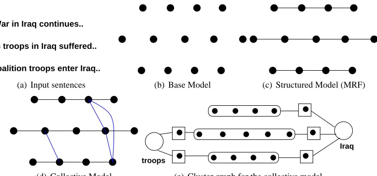
There has been a lot of work on capturing long-range dependencies between labels of non-adjacent words. This typically includes dependencies of the form—if a token repeats in a document, then the labels of the repetitions should ideally be the same (Sutton and McCallum, 2004; Bunescu and Mooney, 2004; Krishnan and Manning, 2006; Finkel et al., 2005). In Figure 1(d), we show an example where the extra dotted edges join unigram recurrences. Such long-range dependencies are termed associative since they introduce positive couplings between labels of token pairs. Apart from textual tokens, associative dependencies have also been exploited while labeling documents (Lu and Getoor, 2003; Chakrabarti et al., 1998), image pixels (Taskar et al., 2004), and annotating Web documents (Kulkarni et al., 2009). Due to these couplings, MAP inference is done collectively across all sentences so as to maximize the sum of sentence-specific and long-range associative potentials. This joint MAP computation task is traditionally called collective inference.
Previous work on collective inference can be broadly classified into two categories. The first category defines a separate associative potential over every inter-instance edge (i.e., dotted edge in Figure 1(d)). Inference on such graphs is performed by viewing it as a graphical model with pairwise potentials. A variety of generic approximation algorithms have been used to solve this typically intractable inference task, including Loopy Belief propagation (Bunescu and Mooney, 2004; Sutton and McCallum, 2004), and Gibbs sampling (Finkel et al., 2005). The second category defines an associative potential for each clique that is created from all repetitions of a unigram and the potentials can take more general forms like the Majority function (Krishnan and Manning, 2006). Collective inference on this category of models is performed using local search algorithms such as Iterative Conditional Mode fitting (ICM) (Lu and Getoor, 2003; Chakrabarti et al., 1998) or two stage algorithms (Krishnan and Manning, 2006).
This paper unifies various collective extraction tasks with different forms of associative poten-tials under a single framework. We do this by employing a cluster graph representation of the collec-tive model. Figure 1(e) illustrates the cluster graph for our toy example. The cluster graph comprises of one cluster per MRF-instance, and one cluster per clique with its corresponding associative po-tential. As in the traditional collective extraction models, we assume that a clique comprises of all the occurrences of a particular token. We emphasize that instead of clusters for chain models, the framework can also define clusters for any tractable component, such as a bipartite matching or an alignment, but since our interest is in IE tasks, we shall focus on chain models.
Collective inference in our model then simply corresponds to message passing in this cluster graph. This view of collective inference offers several advantages over earlier approaches. First, it allows us to plug in and study various clique potentials cleanly under the same cluster message passing umbrella. Second, it allows us to exploit special properties of the associative potentials to design combinatorial algorithms that are both more accurate and more efficient than existing al-gorithms. Specifically, we show that most associative potentials used in practice are symmetric
argu-ments. So the value of a symmetric potential depends only on the counts of its distinct arguments, and not their position in the clique. For example in Figure 1(d), the clique potential on ‘Iraq’ would give a low score if its end vertices had different labels, regardless of which ‘Iraq’ vertex gets what label. We present three families of symmetric clique potentials that capture label associativity in
different ways—MAX, SUM (which subsumes the popular Potts potential), and MAJORITY. The
most crucial component of the collective inference problem is then to efficiently compute outgoing messages from clique clusters governed by symmetric potentials. We denote this sub-problem as
clique inference.
1.1 Contributions
We show that the overall collective inference problem is intractable even for the case of two labels. We therefore concentrate on designing efficient and accurate message passing algorithms on our special cluster graph. We present a suite of efficient combinatorial algorithms tailored to specific symmetric clique potentials for the clique inference sub-problem. We devised a combinatorial al-gorithm calledα-pass that computes exact outgoing messages for cliques withMAXpotentials, and also for any arbitrary symmetric clique potential over two labels. We show thatα-pass provides a 1315-approximation for clique inference with the well-known and NP-hard Potts potential with the
SUMfamily. We show that this analysis is tight, and that the corresponding clique inference bound by alternative schemes likeα-expansion, LP-rounding, TRW-S and ICM are either 12. or at best lo-cally optimal. Further, the runtime ofα-pass is O(mn log n)where n is the clique size, and m is the number of labels. We also show thatα-pass can be generalized to provide a better approximation of
8
9, but with a runtime of O(m
2n log n). Alternative clique inference approaches such as the graph-cut
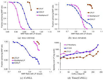
algorithm of Boykov et al. (2001) and the tree-reweighted message passing (TRWS) algorithm of Kolmogorov (2006) are quadratic in n. We present a new Lagrangian-relaxation based algorithm, called LR, forMAJORITYpotentials. The LR algorithm is nearly exact in practice but is usually two orders of magnitude faster than an exact LP-based algorithm.
Our experiments show that computing a rich set of messages leads to significantly more accuracy gains over other collective inference approaches that do not compute such messages, for example, Krishnan and Manning (2006). We also show that decomposing the problem over the cluster graph and employing fast message computation algorithms helps our collective inference scheme converge one-order faster than alternatives like loopy belief propagation. In short, we show that it makes more sense to compute messages at a cluster level, and we provide fast and accurate algorithms to do so.
War in Iraq continues..
US troops in Iraq suffered..
..coalition troops enter Iraq..
(a) Input sentences (b) Base Model (c) Structured Model (MRF)
(d) Collective Model
troops
Iraq
(e) Cluster graph for the collective model
Figure 1: Various models for named-entity recognition illustrated on a small corpus. Figure 1(e) shows the cluster graph for the collective model of (d) with one cluster per sentence (shown as flat chains), and one cluster per associative clique (shown as big circles).
At this point, we note that our previous work (Gupta et al., 2007) focused primarily on theα -pass algorithm along with a sketch of some of its properties. This paper presents a detailed treatment of the algorithm and its generalized version, with rigorous proofs of their approximation bounds, including some new bounds for a variant of the clique inference objective with Potts potential. In addition, new material in this paper includes the LR algorithm for theMAJORITYpotential, exten-sion of our framework to include properties-based associativity, and empirical studies of various collective inference techniques.
We also note that subsequent to our work (Gupta et al., 2007), there has been an abundance of research on higher order clique potentials in last few years, primarily by the computer vision com-munity. While their applications and basic graph structure are different (grids vs chains), many of their ideas are highly relevant—either in terms of special algorithms for clique/collective inference (Komodakis et al., 2007a; Komodakis and Paragios, 2009; Kumar and Torr, 2008a; Werner, 2008), reduction of clique potentials to pairwise potentials (Kohli et al., 2009; Ishikawa, 2009), and special families of clique potentials (Potetz and Lee, 2008; Rother et al., 2009; Tarlow et al., 2010). We will present theoretical and empirical comparisons and draw parallels with the relevant schemes later on in this paper.
1.2 Outline
and analyze their approximation quality. In Section 6, we extend our framework to capture more general associative properties. Section 7 contains experimental results of three types: (a) quality of theα-pass and LR algorithms; (b) effect of modeling more general associative properties in a domain adaptation task; and (c) collective inference via cluster message passing vs alternatives. Fi-nally, Section 8 discusses prior art and Section 9 contains conclusions and a discussion of future work.
2. Collective Inference with MRFs
We now review the basic first-order MRF model for information extraction, and then formally define the collective inference problem over various coupled MRFs. We denote a sentence by bold x, and its labeling vector by y. Consequently, xiand yidenote the ith token in x and its label respectively. The MRF defines a log-linear model parameterized by a weight vector w, where the conditional probability of a labeling is given by:
log P(y|x,w) =
∑
i
φi(yi,yi−1; x,w)−log Zw.
Hereφi(yi,yi−1; w)is the log of the potential on the edge between tokens i and i−1, These potentials
are local, that is, they depend only on the labels of the edge and log Zwis the normalization factor. During inference, we compute the most probable labeling of x:
arg max
y log P(y|x,w) =arg maxy
∑
i φi(yi,yi−1; x,w).If there are m possible labels at each token, and n tokens in x, then exact inference can be done using max-product message passing in O(nm2)time.
We now move to the collective model whose toy example is illustrated in Figure 1(d). Let there be N sentences{x1, . . . ,xN}. Correspondingly, we have N conditional distributions P(yk|xk,w),k= 1, . . . ,N. We use the shorthandφki(yik,yki−1)to refer toφki(yki,yki−1; xk,w).
Let t denote a token that repeats across the sentences, and let
T
denote the set of all such tokens. For a repeating token t, let D(t)be the set of all (sentence-id, token-id) locations where it occurs in the N sentences, that is, D(t) ={(k,i)|xki =t}. We express the conformance in the label assigned to positions in D(t)with a higher order clique potential Ct({yki}(k,i)∈D(t)). Our collective MRF model that couples sentences using unigrams is then given by (up to a normalization constant):log P({yk}Nk=1|{xk}Nk=1,w) ≈
N
∑
k=1log P(yk|xk,w) +
∑
t∈TCt({yki}(k,i)∈D(t)) (1)
≈
N
∑
k=1|xk
|
∑
i=1φk
i(yki,yki−1)
!
+
∑
t∈T
Ct({yki}(k,i)∈D(t)).
The clique potential Ct has two important properties: First, it is invariant under any permutation of its arguments—that is, it is a symmetric function of its input. Thus, if there are m possible labels, we can represent the arguments with an m-bin histogram. For example, if m=3 and input is{1,2,1,1,2,3,2}, then Ct(S)depends on the 3-bin histogram with values 3,3,1. Second, Ct is
associative—that is, it favors agreement of labels in its argument set, and it maximized when all
All collective extraction methods proposed in the literature fit the above framework. The earliest and the most popular collective model used associative potentials over every pair of occurrences of
t (Sutton and McCallum, 2004; Finkel et al., 2005). This pairwise potential was a Potts potential—1
if the pair had matching labels and 0 otherwise. Clearly, we can define an appropriate Ctthat mimics this behavior while staying symmetric. Consider the clique potential:
Ct({yki|(k,i)∈D(t)}) =
∑
(k,i),(l,j)∈D(t)δ(yki =ylj).
This is equivalent to all the pairwise potentials for t. Also, using the histogram view, this can be re-written up to a constant as∑mα=1n2α, where nαis the bin count for labelαin the histogram cor-responding to{yki|(k,i)∈D(t)}. Other known collective models like the ones proposed by Lu and Getoor (2003) and Krishnan and Manning (2006) can also be cast using the ‘Majority’ symmetric clique potential as we shall see in later sections.
Having defined our collective model, and shown that it subsumes popular collective models, we are ready to define the collective inference objective.
Definition 1 (Collective Inference) Collective inference is the task of finding labelings y1, . . . ,yN
that jointly maximize the probability of the collective model (Equation 1):
arg max y1,...,yN
N
∑
k=1|xk|
∑
i=1φk
i(yki,yki−1)
!
+
∑
t∈T
Ct({yki}(k,i)∈D(t)). (2)
In general terms, collective inference corresponds to labeling the nodes of a generic cyclic graph. However, our graph has a special structure—it is composed of chains and cliques, and although the intra-chain edge potentialsφcan be arbitrary, the clique potentials are associative and symmetric. However we next prove that even in this setup, collective inference is NP-hard.
Theorem 2 The collective inference problem is NP-hard even with just two labels.
Proof We reduce the well-known NP-hard problem of finding MAX-CUTs in an arbitrary graph G
to our collective inference problem (called CI). For each node u∈G define a 2-node chain u1u2in
CI where each node can take binary labels and with edge potentialφu(y,y′) =Mδ(y6=y′). M is a large positive number>2E, where E is the number of edges in G. For an edge(u,v)∈G, we add
three cliques:(u1,v1),(u1,v2)and(u2,v1). All three clique potentials are Ct({y,y′}) =δ(y=y′). The key observation is that G has a cut of size≥k iff CI has a map score of≥Mn+E+k where n is the number of nodes in G.
Suppose G has a cut (A,B) of size ≥k. Define a labeling in CI where all variables in A′,
{v1|v∈A} ∪ {v2|v∈B}are labeled 0 and the rest B′ are labeled 1. Then for every u∈G,(u1,u2)
are labeled differently, thus the total contribution from the edge potentials within chains of CI is
Mn. For an edge (u,v)∈G that is part of the cut (A,B) with u∈A,v∈B, two cliques (u1,v2)
and(u2,v1)have both their arguments labeled the same whereas for all other edges only one of the cliques (u1,v1) reaches such conformance. Thus, the total contribution from clique potentials is E+k. The converse holds the same way. Since M is sufficiently large, the edge(u1,u2)in CI will
At this point we note that our collective inference objective is related to various bodies of work on joint inference, primarily in computer vision tasks. For the sake of continuity we defer our discussion of all related work to Section 8 and instead present our framework for maximizing the collective inference objective.
3. Cluster Graph based Collective Inference Framework
Having established that optimizing the objective in Equation 2 is NP-hard, one natural choice for approximating it is ordinary pairwise belief propagation on the collective graphical model. This involves passing messages along edges inside the chains, as well as along the clique edges. How-ever this approach is not suitable due to many reasons. First, some symmetric potentials like the Majority potential cannot be decomposed along the clique edges, so we cannot compute the cor-responding messages. Second, the approach does not exploit the special nature of the clusters and the symmetric potentials. Third, this approach is not tenable if we wish to extend the framework to capture associativities of more general properties of the kind discussed in Section 6.
Hence we adopt message passing on a special cluster graph where every chain and clique cor-responds to a cluster. The clique cluster for a unigram is adjacent to all the chains that contain that unigram, as shown via singleton separator vertices in Figure 1(e). This setup of message passing on the cluster graph allows us to exploit potential-specific algorithms at the cliques, and at the same time work with any arbitrary symmetric clique potentials. Cluster graphs have been used effectively for message passing elsewhere as well (Yedidia et al., 2003; Duchi et al., 2007).
Let mk→t and mt→k denote message vectors from chain k to an incident clique t and vice-versa. A chain is said to be incident on a clique if there exists a position j in chain k which matches term
t, that is,(k,j)∈D(t). We assume that D(t)is created such that from any chain only one position belongs to it. We next discuss how these messages are computed.
3.1 Message from an Instance to a Clique
The message mk→t(y)for a(k,j)∈D(t)is given by:
mk→t(y) = max yk:yk
j=y
|xk|
∑
i=1φk(yk
i,yki−1) +
∑
t′6=t∈T,(k,j′)∈D(t′)
mt′→k(ykj′) !
.
3.2 Message from a Clique to an Instance
The more interesting message computation is that for mt→k given a(k,j)∈D(t). Let the clique t have n vertices. Then the message computation can be written as:
mt→k(y) = max
(y1,...,yk=y,...,yn)(k′,j′)∈
∑
D(t)k′6=kmk′→t(yk′) +Ct({y1, . . . ,yn}). (3)
The maximization in Equation 3 can be re-written as
−mk→t(y) + max
(y1,...,yk=y,...,yn) (k′,j
∑
′)∈D(t)mk′→t(yk′) +Ct({y1, . . . ,yn}) !
. (4)
The maximization term is an instance of the general clique inference problem defined as:
Definition 3 (Clique Inference) Given a clique over n vertices, with a symmetric clique potential C(y1, . . . ,yn), and vertex potentialsψjyfor all j≤n and labels y. Compute a labeling of the clique
vertices that maximizes:
max y1,...,yn
n
∑
j=1ψjyj+C(y1, . . . ,yn). (5)
Thus the second term in Equation 4 can be seen as clique inference by definingψjy,mj→t(y)and C,Ct. To compute mt→k(y), we can solve the clique inference problem with the easily enforceable constraint yk=y. From now on, we refer to outbound message computation at the cliques as clique inference.
4. Symmetric Clique Potentials
Having established cluster message passing as our collective inference paradigm, and clique infer-ence as our message computation tool, we turn our attention towards various families of symmetric clique potentials. As seen in Section 2, these associative clique potentials depend only on the histogram of label counts{ny|y=1, . . . ,m}over the clique, nybeing the number of clique vertices labeled y. Thus for ease of notation, we will denote the arguments of a symmetric potential Ct by ei-ther the vertex labels yt= (y1, . . . ,yn)or by its corresponding count histogram n(yt) = (n1, . . . ,nm). Here we clarify that n is used to denote the entire count histogram, nyto denote the count for label y, while n denotes the clique size. An associative symmetric clique potential is thus maximized when
ny=n for some y, that is, one label is given to all the clique vertices.
We consider specific families of clique potentials, many of which are currently used in real-life tasks. In Section 5 we will look at various potential-specific exact and approximate clique inference algorithms that exploit the specific structure of the potential at a clique.
In particular, we consider the three types of symmetric clique potentials listed in Table 1. They differ in the manner in which they reward skew in the count histogram n.
4.1 MAXClique Potentials
These clique potentials are of the form:
Name Form Remarks
MAX maxy fy(ny) fyis a non-decreasing function.
SUM ∑yfy(ny) fynon-decreasing. Includes Potts =λ∑yn2y.
MAJORITY fa(n), where a=argmaxyny A popular form is fa(n) =∑ywayny.
Table 1: Three kinds of symmetric clique potentials considered in this paper. n= (n1, . . . ,nm) de-notes the counts of various labels among the clique vertices.
for arbitrary non-decreasing functions fy. When fy(ny),ny, we get the makespan clique potential which has roots in the job-scheduling literature. This potential depends only on the biggest label count and ignores the other labels. Truncated version of this potential have been recently used in computer vision (Kohli et al., 2009).
In Section 5.1, we present theα-pass algorithm that computes messages forMAXclique poten-tials exactly in O(mn log n)time. MAXpotentials are tractable and relatively simpler potentials, but
most importantly, they provide key insights to deal with the more complexSUMpotentials.
4.2 SUMClique Potentials
SUMclique potentials are of the form:
C(n1, . . . ,nm) =
∑
yfy(ny).
This family of potentials includes functions that aggregate the histogram skew over bins, for exam-ple, the entropy potential where fy(ny)∝nylog ny. One very interesting member is the case when the well-known Potts model is applied homogeneously on all edges of a clique. Letλ>0 be the pairwise reward of assigning the same label to two nodes of an edge. The summation of these terms over a clique is equivalent (up to a constant) to the clique potential:
CPotts(n1, . . . ,nm) =λ
∑
yn2y.
This corresponds to the gini entropy of the histogram. We will show that the clique inference problem is NP-hard with the above potential and provide a 1315-approximation in Section 5.
We note that the traditional usage of Potts is in a minimization setting, that is, edges are pe-nalized by some costγif their end vertices are labeled differently. The corresponding cost version of Potts is then Cmin(y1, . . . ,yn;γ),γ∑j>iδ(yi6=yj). It is easy to see that these two versions are related by:
CPotts(y1, . . . ,yn;λ) =λn2−Cmin(y1, . . . ,yn; 2λ).
We show that our algorithm provides a32approximation for the minimization version of the problem.
4.3 MAJORITYClique Potentials
AMAJORITYpotential is defined as:
An important special subclass is the linear majority potentials defined as:
CMaj=
∑
y
wayny, a=argmaxyny.
This potential has been used for a variety of tasks such as link-based classification of web-pages (Lu and Getoor, 2003) and named-entity extraction (Krishnan and Manning, 2006). The role of the parameters way is to capture the co-existence of some label pairs in the same clique. Co-existence allows us to downplay ‘strict associativity’ viz. it permits a few cliques vertices to have similar but not necessarily the same labels. For example, consider a clique made from occurrences of the unigram ‘America’. However, some occurrences of America correspond to Location, while others might correspond to an Organization, say Bank of America. Also, it is rare for a location name to be shared with a person name. This can be captured by allowing a higher value of wαy for the (Location, Organization) pair than for the (Location, Person) pair.
Unlike Potts potential, MAJORITY potential cannot be represented using edge potentials. We
will present an exact polynomial time algorithm and several efficient approximations in Section 5.3.
5. Algorithms for Clique Inference
We will use F(y1, . . . ,yn) to denote the clique inference objective in Equation 5. As short-hand, we will denote F(y1, . . . ,yn) by F(y) =ψ(y) +C(y), where ψ(y) is the vertex score (i.e., node potential) of the clique labeling y and the second term is the clique score (i.e., clique potential). Wlog assume that all the vertex termsψiyare positive. Otherwise a constant can be added to all of them and that will not affect the maximization. The MAP clique labeling will be denoted by y∗, and ˆy will denote a possibly sub-optimal labeling.
We show that the clique inference is easy for any C()with just two labels and in Section 5.1 we present an exact algorithm calledα-pass for this case. We show that the same algorithm generalizes to give an exact solution forMAXpotentials. We address theSUMandMAJORITYclique potentials
respectively in Sections 5.2 and 5.3. Finally, in Section 5.4 we show how to extend the clique inference algorithms to efficiently batch the computation of multiple max-marginals.
5.1 α-pass Algorithm
We begin withMAXpotentials. Recall that aMAXpotential is of the form C(n(y)) =maxyfy(ny). We propose an exact inference procedure calledα-pass (Algorithm 1) for such potentials.
The α-pass algorithm guesses that the dominant label in y∗ isα, with a count of k. Of course we do not knowαor k so all(α,k)combinations are tried out. For each(α,k)combination,α-pass computes the best k vertices to assign the labelα. These k vertices are obtained by sorting all the vertices according to the criteriaψ.α−maxβ6=αψ.β, and picking the top-k vertices. Every remaining
vertex u is labeled with the best non-α label as per the vertex score, that is, with arg maxβψuβ. Let ˆyαk denote the clique labeling thus obtained in the(α,k)th combination. Trying out all(α,k) combinations,α-pass returns the ˆyαkwhose score F(ˆyαk)is the highest.
It is straightforward to see that α-pass runs in O(mn log n) time by incrementally computing
F(ˆyαk)from F(ˆyα(k−1)), that is, for eachα, we can sort the vertices just once for all k=1, . . . ,n.
For clique potentials that are decomposable over the edges, as in Potts, this runtime is much better than ordinary belief propagation, which would cost O(m2n2).
Input: Vertex scoresψ, Clique Potential C Output: Labeling ˆy
Best =−∞;
foreach labelα∈ {1, . . . ,m}do
Sort the vertices in descending order according to the metricψ.α−maxβ6=αψ.β;
foreach k∈ {1, . . . ,n}do
Assign the first k sorted vertices the labelα;
Assign the remaining vertices their individual best non-αlabel; s←score of this labeling under F();
if s>Best then
Best←s;
ˆy←current labeling;
end end end return ˆy;
Algorithm 1: Theα-pass algorithm
Claim 5.1 Assignment ˆyαk has the maximum vertex score over all y where k vertices are assigned labelα, that is,ψ(ˆyαk) =maxy:nα(y)=kψ(y).
Claim 5.2 ForMAXpotentials, C(ˆyαk)≥ fα(k).
Proof Labelαhas a count of k and theMAXpotential considers the maximum over all label counts, which is at least k.
Theorem 4 Theα-pass algorithm solves the clique inference problem exactly forMAXclique po-tentials in O(mn log n)time.
Proof Let y∗ be the true MAP and letβ=argmaxyfy(ny(y∗)), ℓ=nβ(y∗). Let ˆy be the labeling returned byα-pass. We have:
F(ˆy) = max
1≤α≤m,1≤k≤nF(ˆy
αk)
≥ F(ˆyβℓ)
= ψ(ˆyβℓ) +C(ˆyβℓ)
≥ ψ(ˆyβℓ) + fβ(ℓ) (by Claim 5.2) = ψ(ˆyβℓ) +C(y∗)
≥ ψ(y∗) +C(y∗) (by Claim 5.1) = F(y∗).
Although we had initially designed the α-pass algorithm forMAX potentials, a similar
argu-ment can be used to show thatα-pass performs exact clique inference for any arbitrary symmetric potential when we have two labels.
Proof Let the MAP y∗ have label counts n1 and n−n1, and a vertex score of ψ(y∗). Let ˆy
be the labeling returned by α-pass. Then we get F(ˆy)≥F(ˆy1n1) =ψ(ˆy1n1) +C(n1,n−n1)≥
ψ(y∗) +C(n1,n−n1) =F(y∗). Since C is arbitrary, the result follows.
We also note that in some real-life tasks the vertex terms tend to heavily dominate the clique term. In such a case too, α-pass will provide an exact solution. This follows immediately from Claim 5.1 and the observation that F(y)≈ψ(y).
5.2 Clique Inference forSUMPotentials
We focus on the Potts potential, the most popular member of the SUM family. Potts potential is
given by CPotts(y) =λ∑yn2y and the clique inference objective is:
max y1,...,yn
n
∑
j=1ψjyj+λ
∑
yn2y. (7)
In the above, λ>0 since we are interested in the associative case which encourages agreement among labels. It is well known that inference with Potts potentials over general graphs, is NP-hard (Boykov et al., 2001) when number of labels is>2 even withλ>0. So we will first show that the task remains NP-hard even for cliques. Then, we will prove thatα-pass achieves an approximation ratio of 45, followed by a more complex proof for a better and tight approximation ratio of 1315. We will then generalize theα-pass algorithm, which will result in an improved ratio of 89 at a cost of higher runtime. In contrast, theα-expansion algorithm of Boykov et al. (2001) will be shown to have a ratio of only 12.
Theorem 5 When C(y) =λ∑yn2y,λ>0, clique inference is NP-hard.
Proof We prove hardness by reduction from the NP-complete Exact Cover by 3-sets problem
(Pa-padimitriou and Steiglitz, 1982). In an instance of Exact Cover by 3-sets, we are given a universe
U of elements, a set S of subsets of U where each subset has three elements, and the goal is to find S′⊆S that covers U , while minimizing|S′|. We create an instance of clique inference as follows. We let elements of U correspond to vertices, and each set in S to a label. Assignψiy=2nλif ele-ment i belongs to set y, and zero otherwise (setλ>0 arbitrarily). Consider the problem of deciding if exactly n3 out of m subsets cover U . The MAP score in the constructed clique inference instance will be(2n2+32 n3)λiff we can find an exact cover.
The above proof establishes that there cannot be an algorithm that is polynomial in both n and m. But we have not ruled out algorithms with complexity that is polynomial in n but exponential in m, say of the form O(2mnk)for a constant k.
We next analyze the approximation guarantees provided by the α-pass algorithm. We first present an easy proof for a weaker bound of 45 and then move on to a more detailed proof for
13
15. Recall that the optimal labeling is y∗and the labeling output byα-pass is ˆy. Theorem 6 F(ˆy)≥4
Proof Without loss of generality assume that the label counts of y∗are n1≥n2≥. . .≥nm. Then
C(y∗) =λ∑yn2y≤λn1∑yny=λnn1.
F(ˆy) ≥ F(ˆy1n1) =ψ(ˆy1n1) +C(ˆy1n1) ≥ ψ(y∗) +C(ˆy1n1) (from Claim 5.1) ≥ ψ(y∗) +λn21 (sinceλ>0)
≥ ψ(y∗) +C(y∗)−λn1n+λn21
≥ F(y∗)−λn2/4. (8)
Now consider the two cases where F(y∗)≥5 4λn
2and F(y∗)<5 4λn
2. For the first case we get from
above that F(ˆy)≥F(y∗)−λn2/4≥4
5F(y∗). For the second case, we know that the score F(ˆy
mn)
where we assign all vertices the last label is at leastλn2(because all vertex scores are assumed to be non-negative) and thus F(ˆy)≥45F(y∗).
We stress that non-negativity of the vertex scores is important for the multiplicative bound of 45, else one can construct examples where F(y∗) =0. At the same time, Equation 8 provides a useful
additive bound that holds for arbitrary vertex scores.
We now state the more involved proof for showing thatα-pass actually provides a tight approx-imation bound of 1315for clique inference with Potts when the vertex scores are non-negative.
Theorem 7 F(ˆy)≥13
15F(y∗). Further, this ratio is tight. Proof See Appendix A.
We next present a generalization of theα-pass algorithm that provides provably better guarantees for Potts.
5.2.1 GENERALIZEDα-PASSALGORITHM
Inα-pass, for each labelα, we go over each count k and find the best vertex score with k vertices assigned labelα. We generalize this to go over all label subsets of size no more than q, a parameter of the algorithm that is fixed based on the desired approximation guarantee.
For each label subset A⊆ {1, . . . ,m} of size no more than q, and for each count k, maximize vertex scores with exactly k vertices assigned a label from A. For this, we sort the vertices in decreasing order of maxα∈Aψiα−maxy6∈Aψiy, assign the top k vertices their best label in A and the remaining their best label not in A. The best solution over all combinations(A,k) with|A| ≤q is
returned as the final labeling ˆy. It is easy to see that this algorithm reduces toα-pass when q=1. The complexity of this algorithm is O(nmqlog n) because there are mq
choices for the set A. In practice, we can use heuristics to prune the number of label subsets. Further, we can make the following claims about the quality of its output.
Theorem 8 Generalizedα-pass enjoys an approximation bound of 89, that is, F(ˆy)≥8 9F(y∗). Proof The bound is achieved with q=2. We provide the details in Appendix A.
5.2.2 α-EXPANSIONALGORITHM
In general graphs, a popular method that provides the approximation guarantee of 1/2 for the Potts model is the graph-cut basedα-expansion algorithm (Boykov et al., 2001). We explore the behavior of this algorithm for clique inference with Potts potentials.
In this scheme, we start with any initial labeling—for example, all vertices are assigned the first label, as suggested in Boykov et al. (2001). Next, for each labelαwe perform anα-expansion phase where we switch the labeling of an optimal set of vertices from their current label toα. We repeat this in a round over the m labels, until no vertices switch their labeling in a complete round.
For graphs whose edge potentials form a metric, an optimalα-expansion move is based on the use of the mincut algorithm of Boykov et al. (2001) which for the case of cliques can be O(n3). We next show how to perform optimalα-expansion moves more efficiently (in O(mn2)time) for all
kinds ofSUMpotentials.
Anα-expansion move: Let ˜y be the labeling at the start of this move. For each label y6=αcreate a sorted list Syof vertices assigned y in ˜y in decreasing order ofψiα−ψiy. If in an optimal move, we move ky vertices from y toα, then it is clear that we need to pick the top ky vertices from Sy. Let ri be the rank of a vertex i in Sy. Our remaining task is to decide the optimal number kyto take from each Sy. We find these using dynamic programming. Without loss of generality assumeα=m. Let
Dj(k)denote the best score when k vertices with current labels in 1. . .j switch toα. We compute
Dj(k) = max
l≤k,l≤nj(˜y)Dj−1(k−l) +fj(nj(˜y)−l) +i′:r
∑
i′≤lψi′α+
∑
i′:ri′>l
ψi′j,
where nj()is the usual cardinality of label j in the labeling. Now we can find the optimal number of vertices to switch toαas argmaxk≤n−nα(˜y)Dm−1(k) +fα(k+nα(˜y)).
5.2.3 COMPARISON WITHEXISTINGAPPROXIMATION BOUNDS
As mentioned earlier, the CPotts clique potential is equivalent to the sum of Potts potentials over edges of a complete graph. For arbitrary graphs with homogeneous Potts potential on edges, the alpha expansion algorithm of Boykov et al. (2001) and the LP relaxation algorithm of Kleinberg and Tardos (2002) provide a factor of 2 approximation guarantee for a minimization version of the objective. For cliques with homogeneous edge potentials, their objective reduces to an energy-based formulation (using their notation):
min y
∑
j
θj(yj) +γ
∑
i,j>iδ(yj6=yi)≡min y
∑
j
θj(yj) +
γ
2(n
2−
∑
y
n2y), (9)
whereθj(yj)denotes node energy and is assumed to be positive andγdenotes the homogeneous Potts parameter.
First we show thatα-expansion provides an approximation bound of 2 even for the special case of cliques. Symmetrically, we also show that the α-expansion algorithm provides a bound of 12 for our original max-version of the clique inference problem. Next, we show thatα-pass provides a bound of 32 for even the minimization objective above. Thus, for both the minimization and maximization objectives,α-pass improves upon the guarantees obtained by existing algorithms.
Proof An instance where this occurs is as follows. There are n nodes and n+1 labels y0, . . . ,yn. The
vertex energy for(xi,y0)is 2n−2 and for(xi,yi)it is 0. All other vertex energies are∞, andγ=1. Suppose initially all nodes are assigned label y0. Then the clique energy is 0 and vertex energy is n(2n−2). Now considering any other label yi,i>=1, the optimal set of nodes to switch is just
xi. But this reduces vertex energy by 2n−2 but increases clique energy by the same amount, so no switching is done. However the optimal solution has xi labeled with yi, which has a total energy of
n2−n.
Theorem 10 Theα-expansion algorithm provides no better approximation guarantee than 1/2 for the maximization objective (7).
Proof Consider an instance where m=√n+1, andλ=1. Letψu1=2√n for all u. Divide the vertices into√n groups of size √n each, and let ψu,i+1=2n for every vertex u in the ith group.
All other vertex scores are zero. Consider the solution where every vertex is assigned label 1. This labeling is locally optimal wrt anyα-expansion move, and its score is n2(1+2/√n). However, the exact solution assigns every vertex group its label, with a score n2(2+1/√n), thus giving a ratio of 1/2 in the limit.
Theorem 11 Theα-pass algorithm achieves an approximation ratio of 32 for the minimization ob-jective 9.
Proof Suppose k=maxynyis the highest count in the optimal labeling. Consider two cases, k≥n/2 and k<n/2.
If k≥n/2, the clique energy is at leastγ(n2−(k2+ (n−k)2)) =γ2k(n−k). The clique energy
inα-pass is at mostγ(2n2−k2−(n−k)) =γ(n−k)(n+k−1). The vertex energy in the optimal labeling cannot be smaller than that inα-pass. Since k>=n/2,(n+k−1)/2k≤3/2.
If k≤n/2, then the clique energy in the optimal labeling is at least γ(n2−nk) =γn(n−k). Therefore the ratio is again at most(n+k−1)/n≤3/2.
As expected, generalizedα-pass provides a superior approximation ratio for Objective 9.
Theorem 12 The generalizedα-pass algorithm with two labels (q=2) achieves an approximation
ratio of 1+
√
2
2 for objective 9.
Proof We omit the complete proof as it is quite detailed and give only a brief sketch. Wlog assume
that 1 and 2 are the two most dominant labels in the optimal labeling OPT, with counts n1,n2≤n1.
Consider two solutions—one given byα-pass (i.e., q=1) when label 1 has count n1, and another
given by generalizedα-pass with q=2 when counts of labels 1 and 2 are n1+n2. The node energies
of these two labelings cannot be worse than that of OPT (Claim 5.1). So the approximation bound depends only on the ratios of the clique energies. Therefore wlog assume thatγ=2 in Objective 9. The clique energies of the two solutions cannot exceed(n2−n2
1)and(n2−
(n1+n2)2
2 )respectively. We
can now work out the two cases whether n21≤(n1+n2)2/2 or not, and get the desired approximation
n1=n/√2 and n2=n−n/
√
2.
5.2.4 ENTROPYPOTENTIALS AND THEα-PASSALGORITHM
As an aside, let us explore the behavior ofα-pass on another family of additive potentials—entropy potentials. Entropy potentials are of the form:
C(n(y)) =λ
∑
y
nylog ny,whereλ>0.
The main reason α-pass provides a good bound for Potts potentials is that it guarantees a clique potential of at least n21where n1is the count of the most dominant label in the optimal solution y∗.
The quadratic term compensates for possible sub-optimality of counts of other labels. If we had a sub-quadratic term instead, say n1log n1for the entropy potentials, the same bound would not have
held. In fact the following theorem shows that for entropy potentials, even thoughα-pass guarantees a clique potential of at least n1log n1, that is not enough to provide a good approximation ratio. Theorem 13 α-pass does not provide a bound better than 12 for entropy potentials.
Proof Consider a counter example where there are m=n+log n labels. Divide the labels into two sets—A with log n labels and B with n labels. The vertex scores are as follows: the vertices are divided into log n chunks of size n/log n each. If the jthvertex lies in the ythchunk, then let it have a vertex score of log n with label y in A and a vertex score of log n+εwith the jthlabel in B. Let all other vertex scores be zero. Also, letλ=1.
Consider the labeling which assigns the yth label in A to the yth chunk. Its score is 2n log n−
n log log n. Now considerα-pass, withα∈A. Initially vertex y will be set to the ythlabel in B. The best labeling found byα-pass will assign every vertex toα, for a total score of roughly n+n log n.
Ifα∈B, then again the best labeling will assign everything toαfor a total score of roughly(n+
1)log n.
Thus the bound is no better than 12 as n→∞.
Thus,α-pass provides good approximations when the clique potential is heavily dominated by the most dominating label. We now look atMAJORITY potentials, which are linear in the counts
{ny}y. Looking at Theorem 13, we expect thatα-pass will not have decent approximation guarantees forMAJORITY. This is indeed the case. We will prove in Section 5.3 that neitherα-pass nor a natural modification ofα-pass enjoy good approximation guarantees.
5.3 Clique Inference forMAJORITYPotentials
Recall that MAJORITYpotentials are of the form C= fa(n), a=argmaxy ny. We consider linear majority potentials where fa(n) =∑ywayny. The matrix W ={wyy′} is not necessarily diagonally dominant or symmetric.
5.3.1 MODIFIEDα-PASSALGORITHM
Assume that we magically know the majority labelαin advance. Then for linear majority potentials, we can incorporate the linear clique term wαyny in the various vertex scores, and this leads to the following natural modifications to theα-pass algorithm: (a) While making iterations for the label
α, sort the vertices according to the modified metricψiα+wαα−maxy6=α(ψiy+wαy), and (b) While sweeping the list forαwith varying values of k, discard all candidate solutions whose majority label is notα.
However even after these modifications,α-pass does not provide the same approximation guar-antee as for homogeneous Potts potentials, as we prove next.
Theorem 14 The modifiedα-pass algorithm cannot have an approximation ratio better than 12 on linear majority potentials with arbitrary W .
Proof Consider the degenerate example where all vertex scores are zero. Letβandγbe two fixed labels and let the matrix W be defined as follows: wβγ=M+ε, wβy=M∀y6=β,γand all the other entries in W are zero.
In modifiedα-pass, whenα6=β, the labeling returned will have a zero score. Whenα=β, all vertices will prefer the label γ, so α-pass will have to assign exactly n/2 vertices to βto make it the majority label, thus returning a score of (M+2ε)n. However, consider the labeling which assigns
n/m vertices to each value, with a score of(m−1)Mn/m. Hence the approximation ratio cannot be
better than12.
5.3.2 EXACTALGORITHM
Since MAJORITY potentials are linear, we can pose the optimization problem in terms of Integer Programs (IPs). Assume that we know the majority labelα. Then, the optimization problem corre-sponds to the IP:
max z
∑
i,y
(ψiy+wαy)ziy,
s.t.∀y :
∑
i
ziy≤
∑
iziα,
∀i :
∑
y
ziy=1, ziy∈ {0,1}. (10)
We can solve m such IPs by guessing various labels as the majority label, and reporting the best overall labeling as the output. However, Equation 10 cannot be tightly relaxed to a linear program. This can be easily shown using a counter example: Consider a 3-vertex, 3-label clique with a zero W matrix. Let the vertex score vectors beψ0= (1,4,0), ψ1= (4,0,4), ψ2= (3,4,0). While solving
This issue can be resolved by making the constraint matrix totally unimodular as follows. Guess the majority labelα, its count k=nα, and solve the following IP:
max z
∑
i,y
(ψiy+wαy)ziy,
s.t.∀y6=α:
∑
iziy≤k,
∑
iziα=k,
∀i :
∑
y
ziy=1, ziy∈ {0,1}. (11)
This IP solves the degree constrained bipartite matching problem, which can be solved exactly in polynomial time. Indeed, it can be shown that the constraint matrix of this IP is totally unimodular, so its LP relaxation will have an integral solution. We refer the reader to Gupta et al. (2009) for the details. Thus we solve O(mn)such problems by varyingαand k, and report the best solution. We believe that the above LP is concave in k, so the system for a fixedαshould be efficiently solvable using golden section search.
5.3.3 LAGRANGIANRELAXATION BASEDALGORITHM FOR MAJORITYPOTENTIALS
Solving the linear system in Equation 11 is very expensive because we need to solve O(mn)LPs, whereas the system in Equation 10 cannot be solved exactly using a linear relaxation. Here, we look at a Lagrangian Relaxation based approach (LR), where we solve the system in Equation 10 but bypass the troublesome constraint∀y6=α:∑iziy≤∑iziα.
We use Lagrangian relaxation to move this constraint to the objective function. Any violation of this constraint is penalized by a positive penalty term. Consider the following modified program, also called the Lagrangian:
L(γ) =L(γ1, . . . ,γm) =max
z
∑
i,y(ψiy+wαy)ziy +∑
y γy(∑
i ziα−∑
i ziy), s.t.∀i :∑
y
ziy=1, ziy∈ {0,1}. (12)
Forγ≥0, and feasible z, L(γ)is an upper bound for our objective in Equation 10. Thus, we compute the lowest such upper bound:
L∗=min
γ≥0L(γ). (13)
Further, the penalty term in Equation 12 is linear in z, so we can merge it with the first term to get another set of modified vertex potentials:
ψα
iy,ψiy+wαy−γy+
∑y′γy′ y=α
0 y6=α .
Equation 12 can now be rewritten in terms ofψα, with the only constraint that z correspond to a valid labeling:
max y
∑
i,yψα
iyziy,
s.t.∀i :
∑
y
Hence, L(γ)can be computed by independently assigning each vertex i to its best label viz. argmaxyψαiy. We now focus on computing L∗. We use an iterative approach, beginning with γ=0, and
carefully choose a new γ at each step to get a non-increasing sequence of L(γ)’s. We describe the method of choosing a newγlater in this section, and instead outline sufficient conditions for termination and detection of optimality.
Theorem 15 z∗andγ∗are optimum solutions to Equations 10 and 13 respectively if they satisfy the conditions:
∀y :
∑
i
z∗iy≤
∑
i
z∗iα, (14)
∀y : |γ∗y(
∑
i
z∗iy−
∑
i
z∗iα)|=0. (15)
Theorem 15 holds only for fractional z∗. To see how, consider an example with three vertices and two labels. Letψi1+wα1>ψi2+wα2 for all i andα. During Lagrangian relaxation withα=2,
initiallyγ=1 will cause all vertices to be assigned label 1, violating Equation 14. Since the count
difference ∑izi1−∑izi2 ∈ {±1,±2,±3}, any non-zero γ1 will violate Equation 15. Subsequent
reduction ofγ1to zero will again cause the original violation of Equation 14. Consequently, one of
Equations 14 and 15 will never be satisfied and the algorithm will oscillate.
To tackle this, we relax Equation 15 to|γy(∑iz∗iy−∑iz∗iα)| ≤ε, whereεis a small fraction of an upper bound onγy. This helps in reporting labelings that respect the majority constraint in Equation 14 and are close to the optimal.
The outline of the algorithm is described in Figure 2.
We now discuss a somewhat conservative approach to select a new γ at every step. We ini-tially attempted subgradient optimization and golden search to compute step direction and sizes for changingγ. However, we ran into various practical difficulties. Subgradient optimization required very careful tweaking of the step size across iterations, an issue exacerbated by the discrete na-ture of our problem. On the other hand, golden search was too aggressive in practice, leading to many avoidable label flips and consequently many more iterations. So instead we implemented a conservative approach which we describe next.
5.3.4 CONSERVATIVECOORDINATEDESCENT
We perform conservative coordinate descent which avoids large changes and thus too many label flips. Let y be the worst violating label in the current iteration. We will first consider the case when its count exceeds that ofα, so that Equation 14 does not hold.
To decrease the count of y, we need to increase γy. Let i be a vertex currently assigned y and let β(i) be its second most preferred label under the vertex potentials ψαi. The vertex j=
argmaxi:ziy=1ψαiβ(i)−ψαiyis the easiest to flip. So we increaseγyjust enough to make this flip happen. The new value ofγyis therefore given by:
γy= min i:ziy=1
∆ψ
(i,y,β(i)) +γβ(i) β(i)6=α
1
assigned y may also move toα. However since the change is conservative, we expect this behavior to be limited. In our experiments, we found that this conservative scheme converges much faster than golden search over a variety of data.
We now look at the case when Equation 14 is satisfied by all labels but Equation 15 is violated by some label y. In this scenario, we need to decreaseγyto decrease the magnitude of the violation. Here too, we conservatively decreaseγybarely enough to flip one vertex to y. If i is any vertex not assigned label y andβ(i)is its current label, then the new value ofγyis given by:
γy= max i:ziy6=1
∆ψ
(i,y,β(i)) +γβ(i) β(i)6=α
1
2(∆ψ(i,y,α)−∑y′6=yγy′) β(i) =α . (17) Note that the arguments of Equations 16 and 17 are the same. In this case too, in spite of a conser-vative move, more than one vertex markedαmay flip to some other value, although at most one of them will be flipped to y. As before, the small magnitude of the change restricts this behavior in practice.
Input:ψ,W,α,maxIters,tolerance Output: approximately best assignment ˆy
γ←0;
iter←0;
ˆz←Assignment with all vertices assignedα;
while iter<maxIters do
Compute L(γ) (Equation 12), let z be the solution;
if F(z)>F(ˆz)then
ˆz←z; end
(y,∆)←Worst violator and violation (Equations 14 and 15);
if∆ <tolerance then
We are done, L∗=L(γ);
break; else
Modifyγyusing conservative coordinate descent; end
iter←iter+1;
end
Construct assignment ˆy from ˆz;
return ˆy
Algorithm 2: LR Algorithm for Majority potentials
5.4 Computing All Node Max-marginals
In this section, we discuss an important optimization that speeds up message-passing in a cluster graph. We show that for symmetric potentials we can compute max-marginals in O(m2)calls to the clique inference algorithm in practice, as opposed to the expected nm invocations. Cliques can be arbitrarily big, so removing the dependence on n is very helpful in practice.
Our basic strategy is as follows. For label pairsα,β, define a modified clique potential function Cαβthat adds “1” to the count for labelβand subtracts “1” from the count of labelα:
Find MAP labeling yαβ using the modified scoring function Fαβ(y) =ψ(y) +Cαβ(y). Let v be a vertex whose label in yαβ isα, then the max marginal Mvβ,maxy:yv=βF(y) =Fαβ(yαβ)−ψvα+
ψvβ. The outgoing message mt→v(β)is then simply Mvβ−mv→t(β)as per Equation 4. A proof of correctness of this optimization is as follows.
Theorem 16 maxy:yv=βF(y) =Fαβ(yαβ)−ψvα+ψvβ.
Proof
max
y Fαβ(y) = y:yvmax=αFαβ(y) since v is labeledαin y αβ
= max
y:yv=αψ(y) +Cαβ(y)
= max
y:yv=βψ(y)−ψvβ+ψvα+C(y)
= max
y:yv=βF(y)−ψvβ+ψvα.
We invoke the above strategy for all label pairsα,βwhen some vertex in the original MAP gets labelα. There is no guarantee that all nm messages would be generated by the above scheme. The ones that are not covered are computed using separate invocations of MAP.
This concludes the description of our various clique inference algorithms and their theoret-ical properties. The discussion until now had focused on the traditional unigram-clique collec-tive inference model. We now switch tracks and describe an extension of the colleccollec-tive inference framework—one which captures richer kinds of associativity that is often present in the data. We will see that the same cluster message passing setup and collective inference algorithms can be used almost as is in this more general scenario.
6. Properties-based Collective Inference Framework
We broaden the notion of collective inference to encourage richer forms of associativity amongst the labelings of multiple records. This more general framework has applications in domain adaptation. We illustrate this via an example.
Example: Consider extracting bibliographic information from an author’s publications homepage
using a model trained on a different set of pages. The labels of interest are Title, Author, Venue, and Date. Typically, within each homepage (a domain) we expect consistency in the style of individual publication records. For example, we expect the following properties to be largely uni-valued inside a domain:
1. The ordering of labels in the labelings (e.g., Title→Author*→Venue).
2. The token preceding the Title, or ‘Start’ if Title occurs at the beginning.
3. The label appearing after the Venue, or ‘End’ if Venue occurs at the end.
A Simulator for estimating Railway Line Capacity.
In APORS - 2003.
(Start, Date,<b>) Bhardwaj, P. (2001). Delegating Pricing Decisions.
Marketing Science 20(2). 143-169.
(‘.’, Volume,<li>)
Scheduling Loosely Connected Task Graphs.
Jour-nal of Computer and System Sciences , August 2003
.
(Start, Date,<b>) Balasubramaniam, S. and P. Bhardwaj (2004). When
not all conflict is bad: Manufacturing marketing con-flict and strategic incentive design. Management
Sci-ence 50(4). 489-502.
(‘.’, Volume,<li>)
Devanagari Pen-written Character Recognition. In
ADCOM - 2001 .
(Start, Date,<b>) Bhardwaj, P. and S. Balasubramaniam (2005).
Man-aging Channel Profits: The Role of Managerial Incen-tives. Forthcoming Quantitative Marketing and
Eco-nomics.
(‘.’, End,<li>)
Table 2: Two publications pages with different styles. Text in parentheses shows the values of three properties on the correct labelings: (i) Token before Title (ii) First non-Other label after Venue (iii) HTML tag containing Title. The properties are largely uni-modal inside a page, but the mode varies across pages.
Note that ‘IEEE’ will tend to recur across multiple records, so the last property corresponds to the unigram-based cliques that we modeled thus far. It is clear now that we can gain a lot more if we couple the records together according to ‘richer’ properties than just unigrams.
Of course the choice of properties is crucial. For all the properties illustrated above, we expect that the labelings inside the domain agree on the property value, without caring for what the value actually is (which varies from domain to domain). This allows us to use the same property on different domains, with varying formatting and authoring styles. Table 2 illustrates this for two publications pages with different styles. It shows three properties that take on largely similar values across records inside a domain, but the dominant value changes across domains. Thus we can reward associativity of these property values using the same symmetric potentials that we have used for unigram cliques.
Now assume that we have an array of such conformance-promoting properties, and a basic MRF trained on some labeled domains. An effective way of deploying this MRF on a previously unseen domain is by labeling the records in the new domain collectively while encouraging the individual labelings to agree on our set of properties. If the properties continue to remain associative in the unseen domain, then collective inference can be expected to correct a significant number of errors. This provides us with an inference-only approach, in contrast to many existing solutions for domain adaptation which require model re-training (Blei et al., 2002; Blitzer et al., 2006; Mann and McCallum, 2007).
We now give an intuitive description of how the introduction of properties causes only minor changes in our collective inference framework. The modified collective inference objective is now given by:
arg max y1,...,yN
N
∑
k=1|xk|
∑
i=1φk
i(yki,yki−1)
!
+
∑
g∈G
Cg({g(xk,yk)}k),
instead of Equation 2. Here