Risk Bounds for the Majority Vote: From a PAC-Bayesian
Analysis to a Learning Algorithm
Pascal Germain [email protected]
Alexandre Lacasse [email protected]
Fran¸cois Laviolette [email protected]
Mario Marchand [email protected]
Jean-Francis Roy [email protected]
D´epartement d’informatique et de g´enie logiciel Universit´e Laval
Qu´ebec, Canada, G1V 0A6
?All authors contributed equally to this work.
Editor:Koby Crammer
Abstract
We propose an extensive analysis of the behavior of majority votes in binary classification. In particular, we introduce a risk bound for majority votes, called theC-bound, that takes into account the average quality of the voters and their average disagreement. We also propose an extensive PAC-Bayesian analysis that shows how theC-bound can be estimated from various observations contained in the training data. The analysis intends to be self-contained and can be used as introductory material to PAC-Bayesian statistical learning theory. It starts from a general Bayesian perspective and ends with uncommon PAC-Bayesian bounds. Some of these bounds contain no Kullback-Leibler divergence and others allow kernel functions to be used as voters (via the sample compression setting). Finally, out of the analysis, we propose the MinCq learning algorithm that basically minimizes the C-bound. MinCq reduces to a simple quadratic program. Aside from being theoretically grounded, MinCq achieves state-of-the-art performance, as shown in our extensive empirical comparison with both AdaBoost and the Support Vector Machine.
Keywords: majority vote, ensemble methods, learning theory, PAC-Bayesian theory, sample compression
1. Previous Work and Implementation
This paper can be considered as an extended version of Lacasse et al. (2006) and Laviolette et al. (2011), and also contains ideas from Laviolette and Marchand (2005, 2007) and Ger-main et al. (2009, 2011). We unify this previous work, revise the mathematical approach, add new results and extend empirical experiments.
The source code to compute the various PAC-Bayesian bounds presented in this paper and the implementation of the MinCq learning algorithm is available at:
2. Introduction
In binary classification, many state-of-the-art algorithms output prediction functions that can be seen as a majority vote of “simple” classifiers. Firstly, ensemble methods such as Bagging (Breiman, 1996), Boosting (Schapire and Singer, 1999) and Random Forests (Breiman, 2001) are well-known examples of learning algorithms that output majority votes. Secondly, majority votes are also central in the Bayesian approach (see Gelman et al., 2004, for an introductory text); in this setting, the majority vote is generally called the Bayes Classifier. Thirdly, it is interesting to point out that classifiers produced by kernel methods, such as the Support Vector Machine (SVM) (Cortes and Vapnik, 1995), can also be viewed as majority votes. Indeed, to classify an examplex, the SVM classifier computes
sgn
|S|
X i=1
αiyik(xi, x)
, (1)
wherek(·,·) is a kernel function, and the input-output pairs (xi, yi) represent the examples
from the training setS. Thus, one can interpret each yik(xi,·) as a voter that chooses (with
confidence level|k(xi, x)|) between two alternatives (“positive” or “negative”), andαias the
respective weight of this voter in the majority vote. Then, if the total confidence-multiplied weight of each voter that votes positive is greater than the total confidence-multiplied weight of each voter that votes negative, the classifier outputs a +1 label (and a −1 label in the opposite case). Similarly, each neuron of the last layer of an artificial neural network can be interpreted as a majority vote, since it outputs a real value given byK(P
iwigi(x)) for
someactivation function K.1
In practice, it is well known that the classifier output by each of these learning algorithms performs much better than any of its voters individually. Indeed, voting can dramatically improve performance when the “community” of classifiers tends to compensate for individual errors. In particular, this phenomenon explains the success of Boosting algorithms (e.g., Schapire et al., 1998). The first aim of this paper is to explore how bounds on the generalized risk of the majority vote are not only able to theoretically justify learning algorithms but also to detect when the voted combination provably outperforms the average of its voters. We expect that this study of the behavior of a majority vote should improve the understanding of existing learning algorithms and even lead to new ones. We indeed present a learning algorithm based on these ideas at the end of the paper.
The PAC-Bayesian theory is a well-suited approach to analyze majority votes. Initiated by McAllester (1999), this theory aims to provide Probably Approximately Correct guar-antees (PAC guarguar-antees) to “Bayesian-like” learning algorithms. Within this approach, one considers aprior2 distributionP over a space of classifiers that characterizes its prior belief about good classifiers (before the observation of the data) and a posterior distribution Q
(over the same space of classifiers) that takes into account the additional information pro-vided by the training data. The classical PAC-Bayesian approach indirectly bounds the risk
1. In this case, each votergi has incoming weights which are also learned (often by back propagation of
errors) together with the weightswi. The analysis presented in this paper considers fixed voters. Thus,
the PAC-Bayesian theory for artificial neural networks remains to be done. Note however that the recent work by McAllester (2013) provides a first step in that direction.
of a Q-weighted majority vote by bounding the risk of an associate (stochastic) classifier, called the Gibbs classifier. A remarkable result, known as the “PAC-Bayesian Theorem”, provides a risk bound for the “true” risk of the Gibbs classifier, by considering the empir-ical risk of this Gibbs classifier on the training data and the Kullback-Leibler divergence between a posterior distribution Q and a prior distribution P. It is well known (Lang-ford and Shawe-Taylor, 2002; McAllester, 2003b; Germain et al., 2009) that the risk of the (deterministic) majority vote classifier is upper-bounded by twice the risk of the associ-ated (stochastic) Gibbs classifier. Unfortunately, and especially if the involved voters are weak, this indirect bound on the majority vote classifier is far from being tight, even if the PAC-Bayesian bound itself generally gives a tight bound on the risk of the Gibbs classifier. In practice, as stated before, the “community” of classifiers can act in such a way as to compensate for individual errors. When such compensation occurs, the risk of the majority vote is then much lower than the Gibbs risk itself and, a fortiori, much lower than twice the Gibbs risk. By limiting the analysis to Gibbs risk only, the commonly used PAC-Bayesian framework is unable to evaluate whether or not this compensation occurs. Consequently, this framework cannot help in producing highly accurate voted combinations of classifiers when these classifiers are individually weak.
In this paper, we tackle this problem by studying the margin of the majority vote as a random variable. The first and second moments of this random variable are respectively linked with the risk of the Gibbs classifier and the expected disagreement between the voters of the majority vote. As we will show, the well-known factor of two used to bound the risk of the majority vote is recovered by applying Markov’s inequality to the first moment of the margin. Based on this observation, we show that a tighter bound, that we call theC-bound, is obtained by considering the first two moments of the margin, together with Chebyshev’s inequality.
Section 4 presents, in a more detailed way, the work on theC-bound originally presented in Lacasse et al. (2006). We then present both theoretical and empirical studies that show that theC-bound is an accurate indicator of the risk of the majority vote. We also show that theC-bound can be smaller than the risk of the Gibbs classifier and can even be arbitrarily close to zero even if the risk of the Gibbs classifier is close to 1/2. This indicates that theC-bound can effectively capture the compensation of the individual errors made by the voters.
Sections 6 and 7 bring together relatively new PAC-Bayesian ideas that allow us, for one part, to derive a PAC-Bayesian bound that does not rely on the Kullback-Leibler divergence between the prior and posterior distributions (as in Catoni, 2007; Germain et al., 2011; Laviolette et al., 2011) and, for the other part, to extend the bound to the case where the voters are defined using elements of the training data,e.g., voters defined by kernel functions
yik(xi,·). This second approach is based on the sample compression theory (Floyd and
Warmuth, 1995; Laviolette and Marchand, 2007; Germain et al., 2011). In PAC-Bayesian theory, the sample compression approach is a priori problematic, since a PAC-Bayesian bound makes use of a prior distribution on the set of all voters that has to be defined before observing the data. If the voters themselves are defined using a part of the data, there is an apparent contradiction that has to be overcome.
Based on the foregoing, a learning algorithm, that we call MinCq, is presented in Sec-tion 8. The algorithm basically minimizes theC-bound, but in a particular way that is, inter alia, justified by the PAC-Bayesian analysis of Sections 6 and 7. This algorithm was origi-nally presented in Laviolette et al. (2011). Given a set of voters (either classifiers or kernel functions), MinCq builds a majority vote classifier by finding the posterior distribution Q
on the set of voters that minimizes the C-bound. Hence, MinCq takes into account not only the overall quality of the voters, but also their respective disagreements. In this way, MinCq builds a “community” of voters that can compensate for their individual errors. Even though the C-bound consists of a relatively complex quotient, the MinCq learning algorithm reduces to a simple quadratic program. Moreover, extensive empirical experi-ments confirm that MinCq is very competitive when compared with AdaBoost (Schapire and Singer, 1999) and the Support Vector Machine (Cortes and Vapnik, 1995).
In Section 9, we conclude by pointing out recent work that uses the PAC-Bayesian theory to tackle more sophisticated machine learning problems.
3. Basic Definitions
We consider classification problems where the input space X is an arbitrary set and the output space is a discrete set denotedY. Anexample (x, y) is an input-output pair where
x ∈ X and y ∈ Y. A voter is a function X → Y for some output space Y related to Y. Unless otherwise specified, we consider the binary classification problem whereY ={−1,1} and then we either consider Y as Y itself, or its convex hull [−1,+1]. In this paper, we also use the following convention: f denotes a real-valued voter (i.e., Y = [−1,1]), and h
denotes a binary-valued voter (i.e., Y ={−1,1}). Note that this notion of voters is quite general, since any uniformly bounded real-valued set of functions can be viewed as a set of voters when properly normalized.
We consider learning algorithms that construct majority votes based on a (finite) setH
of voters. Given any x∈ X, the output BQ(x) of aQ-weighted majority vote classifier BQ
(sometimes called theBayes classifier) is given by
BQ(x)
def = sgn
E
f∼Qf(x)
, (2)
Thus, in case of a tie in the majority vote – i.e., Ef∼Qf(x) = 0 –, we consider that the
majority vote classifier abstains –i.e.,BQ(x) = 0. There are other possible ways to handle
this particular case. In this paper, we choose to define sgn(0) = 0 because it simplifies the forthcoming analysis.
We adopt the PAC setting where each example (x, y) is drawn i.i.d. according to a fixed, but unknown, probability distribution Don X ×Y. The training set of m examples is denoted by S = h(x1, y1), . . . ,(xm, ym)i ∼ Dm. Throughout the paper, D0 generically
represents either the true (and unknown) distribution D, or its empirical counterpart US
(i.e., the uniform distribution over the training setS). Moreover, for notational simplicity, we often replace US by S.
In order to quantify the accuracy of a voter, we use a loss function L : Y ×Y →[0,1].
The PAC-Bayesian theory traditionally considers majority votes of binary voters of the form
h : X → {−1,1}, and the zero-one loss L01 h(x), y
def
= I h(x) 6= y
, where I(a) = 1 if predicateais true and 0 otherwise.
The extension of the zero-one loss to real-valued voters (of the form f :X →[−1,1]) is given by the following definition.
Definition 1 In the (more general) case where voters are functions f :X → [−1,1], the zero-one loss L01 is defined by
L01 f(x), y
def
= I y·f(x)≤0 .
Hence, a voter abstention –i.e., whenf(x) outputs exactly 0 – results in a loss of 1. Clearly, other choices are possible for this particular case.3
In this paper, we also consider the linear loss L` defined as follows.
Definition 2 Given a voter f :X →[−1,1], the linear loss L` is defined by
L` f(x), y
def
= 1 2
1−y·f(x)
.
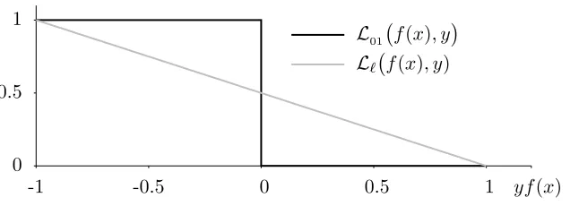
Note that the linear loss is equal to the zero-one loss when the output space is binary. That is, for any (h(x), y)∈ {−1,1}2, we always have
L` h(x), y
= L01 h(x), y
, (3)
because L` h(x), y= 1 ifh(x)6=y, and L` h(x), y= 0 ifh(x) =y. Hence, we generalize
all definitions implying classifiers to voters using the equality of Equation (3) as an inspi-ration. Figure 1 illustrates the difference between the zero-one loss and the linear loss for real-valued voters. Remember that in the casey f(x) = 0 , the loss is 1 (see Definition 1).
Definition 3 Given a loss function L and a voterf, theexpected loss ELD0(f) off relative
to distributionD0 is defined as
ELD0(f)
def
= E
(x,y)∼D0 L f(x), y
.
0 0.5 1
-1 -0.5 0 0.5 1 yf(x)
L01 f(x), y
L` f(x), y)
Figure 1: The zero-one loss L01 and the linear lossL` as a function ofyf(x).
In particular, the empirical expected loss on a training set S is given by
ELS(f) =
1
m
m
X
i=1
L f(xi), yi.
We therefore define the risk of the majority voteRD0(BQ) as follows.
Definition 4 For any probability distributionQon a set of voters, theBayes risk RD0(BQ),
also calledrisk of the majority vote, is defined as the expected zero-one loss of the majority vote classifierBQ relative toD0. Hence,
RD0(BQ) def= EL01
D0 (BQ) = E
(x,y)∼D0 I
BQ(x)6=y
= E
(x,y)∼D0 I
E
f∼Q y·f(x)≤0
.
Remember from the definition ofBQ(Equation 2) that the majority vote classifier abstains
in the case of a tie on an example (x, y). Therefore, the above Definition 4 implies that the Bayes risk is 1 in this case, as Rh(x,y)i(BQ) =L01(0, y) = 1. In practice, a tie in the vote is a
rare event, especially if there are many voters.
The output of the deterministic majority vote classifier BQ is closely related to the
output of a stochastic classifier called the Gibbs classifier. To classify an input example x, the Gibbs classifier GQ randomly chooses a voterf according toQand returnsf(x). Note
the stochasticity of the Gibbs classifier: it can output different values when given the same input x twice. We will see later how the link between BQ and GQ is used in the
PAC-Bayesian theory.
In the case of binary voters, the Gibbs risk corresponds to the probability that GQ
misclassifies an example of distributionD0. Hence,
RD0(GQ) = Pr
(x,y)∼D0
h∼Q
h(x)6=y
= E
h∼QE L01
D0 (h) = E
(x,y)∼D0 h∼EQI h(x)6=y
.
In order to handle real-valued voters, we generalize the Gibbs risk as follows.
Definition 5 For any probability distributionQon a set of voters, theGibbs risk RD0(GQ)
is defined as the expected linear loss of the Gibbs classifier GQ relative toD0. Hence,
RD0(GQ) def= E
f∼QE L`
D0(f) =
1 2
1− E
(x,y)∼D0 fE∼Qy·f(x)
Remark 6 It is well known in the PAC-Bayesian literature (e.g., Langford and Shawe-Taylor, 2002; McAllester, 2003b; Germain et al., 2009) that the Bayes risk RD0(BQ) is
bounded by twice the Gibbs risk RD0(GQ). This statement extends to our more general
definition of the Gibbs risk (Definition 5).
Proof Let (x, y)∈ X × {−1,1} be any example. We claim that
Rh(x,y)i(BQ) ≤ 2Rh(x,y)i(GQ). (4)
Notice thatRh(x,y)i(BQ) is either 0 or 1 depending of the fact thatBQ errs or not on (x, y).
In the case where Rh(x,y)i(BQ) = 0, Equation (4) is trivially true. If Rh(x,y)i(BQ) = 1, we
know by the last equality of Definition 4 that E
f∼Qy·f(x)≤0. Therefore, Definition 5 gives
2·Rh(x,y)i(GQ) = 2·
1 2
1− E
f∼Qy·f(x)
≥ 1 =Rh(x,y)i(BQ),
which proves the claim.
Now, by taking the expectation according to (x, y) ∼D0 on each side of Equation (4), we obtain
RD0(BQ) = E
(x,y)∼D0 Rh(x,y)i(BQ) ≤ (x,yE)∼D0 2Rh(x,y)i(GQ) = 2RD 0(GQ),
as wanted.
Thus, PAC-Bayesian bounds on the risk of the majority vote are usually bounds on the Gibbs risk, multiplied by a factor of two. Even if this type of bound can be tight in some situations, the factor two can also be misleading. Langford and Shawe-Taylor (2002) have shown that under some circumstances, the factor of two can be reduced to (1 +). Nevertheless, distributions Q on voters giving RD0(GQ) RD0(BQ) are common. The
extreme case happens when the expected linear loss on each example is just below one half – i.e., for all (x, y),Ef∼Q y f(x) = 12−–, leading to a perfect majority vote classifier but
an almost inaccurate Gibbs classifier. Indeed, we haveRD0(GQ) = 1
2−and RD0(BQ) = 0. Therefore, in this circumstance, the bound RD0(BQ) ≤ 1−2, given by Remark 6, fails to
represent the perfect accuracy of the majority vote. This problem is due to the fact that the Gibbs risk only considers the loss of the average output of the population of voters. Hence, the bound of Remark 6 states that the majority vote is weak whenever every individual voter is weak. The bound cannot capture the fact that it might happen that the “community” of voters compensates for individual errors. To overcome this lacuna, we need a bound that compares the output of voters between them, not only the average quality of each voter taken individually.
We can compare the output of binary voters by considering the probability of disagree-ment between them:
Pr
x∼D0 X
h1,h2∼Q
h1(x)6=h2(x)
= E
x∼D0 X
E
h1∼Qh2∼EQI
h1(x)6=h2(x)
= E
x∼D0 X
E
h1∼Q
E
h2∼Q
Ih1(x)·h2(x)6= 1
= E
x∼D0 X
E
h1∼Qh2∼EQL01 h1(x)·h2(x),1
where D0
X denotes the marginal on X of distribution D0. Definition 7 extends this notion
of disagreement to real-valued voters.
Definition 7 For any probability distribution Q on a set of voters, theexpected disagree-ment dD0
Q relative to D0 is defined as
dD0
Q
def
= E
x∼D0 X
E
f1∼Q
E
f2∼Q L
` f1(x)·f2(x),1
= 1 2
1− E
x∼D0 X
E
f1∼Q f2∼EQ1·f1(x)·f2(x)
= 1 2
1− E
x∼D0 X
E
f∼Qf(x)
2 .
Notice that the value of dD0
Q does not depend on the labelsy of the examples (x, y) ∼D0.
Therefore, we can estimate the expected disagreement with unlabeled data.
4. Bounds on the Risk of the Majority Vote
The aim of this section is to introduce the C-bound, which upper-bounds the risk of the majority vote (Definition 4) based on the Gibbs risk (Definition 5) and the expected dis-agreement (Definition 7). We start by studying the margin of a majority vote as a random variable (Section 4.1). From the first moment of the margin, we easily recover the well-known bound of twice the Gibbs risk presented by Remark 6 (Section 4.2). We therefore suggest extending this analysis to the second moment of the margin to obtain theC-bound (Section 4.3). Finally, we present some statistical properties of the C-bound (Section 4.4) and an empirical study of its predictive power (Section 4.5).
4.1 The Margin of the Majority Vote and its Moments
The bounds on the risk of a majority vote classifier proposed in this section result from the study of the weighted margin of the majority vote as a random variable.
Definition 8 Let MD0
Q be the random variable that, given any example (x, y) drawn
ac-cording toD0, outputs the margin of the majority voteBQ on that example, which is
MQ(x, y)
def = E
f∼Q y·f(x).
From Definitions 4 and 8, we have the following nice property:4
RD0(BQ) = Pr
(x,y)∼D0
MQ(x, y)≤0
. (5)
4. Note that for another choice of the zero-one loss definition (Definition 1), the tie in the majority vote –
i.e., whenMQ(x, y) = 0 – would have been more complicated to handle, and the statement should have
been relaxed to
Pr (x,y)∼D0
MQ(x, y)<0
≤ RD0(BQ) ≤ Pr
(x,y)∼D0
MQ(x, y)≤0
The margin is not only related to the risk of the majority vote, but also to Gibbs risk. For that purpose, let us consider the first moment µ1(MD
0
Q ) of the random variable MD
0
Q
which is defined as
µ1(MD
0
Q )
def
= E
(x,y)∼D0 MQ(x, y). (6)
We can now rewrite the Gibbs risk (Definition 5) as a function of µ1(MD0
Q ), since
RD0(GQ) = E
f∼QE L`
D0(f) =
1 2
1− E
(x,y)∼D0 fE∼Q y·f(x)
= 1 2
1− E
(x,y)∼D0MQ(x, y)
= 1 2
1−µ1(MD
0
Q )
. (7)
Similarly, we can rewrite the expected disagreement as a function of the second moment of the margin. We use µ2(MD
0
Q ) to denote the second moment. Since y ∈ {−1,1} and,
therefore, y2 = 1, the second moment of the margin does not rely on labels. Indeed, we have
µ2(MD0
Q )
def
= E
(x,y)∼D0 h
MQ(x, y)
i2
(8)
= E
(x,y)∼D0 y
2·h E
f∼Q f(x)
i2
= E
x∼D0 X
h
E
f∼Q f(x)
i2 .
Hence, from the last equality and Definition 7, the expected disagreement can be expressed as
dD0
Q =
1 2
1− E
x∼D0 X
E
f∼Qf(x)
2
= 1 2
1−µ2(MD0
Q )
. (9)
Equation (9) shows that 0 ≤ dD0
Q ≤ 1/2, since 0 ≤ µ2(MD
0
Q ) ≤ 1. Furthermore, we
can upper-bound the disagreement more tightly than simply saying it is at most 1/2 by making use of the value of the Gibbs risk. To do so, let us write the variance of the margin as
Var(MD0
Q )
def
= Var
(x,y)∼D0 MQ(x, y)
= µ2(MD
0
Q ) − µ1(MD
0
Q )
2
. (10)
Therefore, as the variance cannot be negative, it follows that
µ2(MD0
Q ) ≥ µ1(MD
0
Q )
which implies that
1−2·dD0
Q ≥ (1−2·RD0(GQ))
2 . (11)
Easy calculation then gives the desired bound of dD0
Q (that is based on the Gibbs risk):
dD0
Q ≤ 2·RD0(GQ)· 1−RD0(GQ). (12)
We therefore have the following proposition.
Proposition 9 For any distribution Q on a set of voters and any distribution D0 on
X ×{−1,1}, we have
dD0
Q ≤ 2·RD0(GQ)· 1−RD0(GQ) ≤ 1
2.
Moreover, if dD0
Q = 12 then RD0(GQ) = 1 2.
Proof Equation (12) gives the first inequality. The rest of the proposition directly fol-lows from the fact thatf(x) = 2x(1−x) is a parabola whose (unique) maximum is at the point (12,12).
4.2 Rediscovering the bound RD0(BQ)≤2·RD0(GQ)
The well-known factor of two with which one can transform a bound on the Gibbs risk
RD0(GQ) into a bound on the risk RD0(BQ) of the majority vote is usually justified by
an argument similar to the one given in Remark 6. However, as shown by the proof of Proposition 10, the result can also be obtained by considering that the risk of the majority vote is the probability that the marginMD0
Q is lesser than or equal to zero (Equation 5) and
by simply applying Markov’s inequality (Lemma 46, provided in Appendix A).
Proposition 10 For any distribution Q on a set of voters and any distribution D0 on
X ×{−1,1}, we have
RD0(BQ) ≤ 2·RD0(GQ).
Proof Starting from Equation (5) and using Markov’s inequality (Lemma 46), we have
RD0(BQ) = Pr
(x,y)∼D0 MQ(x, y)≤0
= Pr
(x,y)∼D0 1−MQ(x, y)≥1
≤ E
(x,y)∼D0 1−MQ(x, y)
(Markov’s inequality)
= 1− E
(x,y)∼D0 MQ(x, y) = 1−µ1(MD
0
Q ) = 2·RD0(GQ).
0 0.2 0.4 0.6 0.8 1 Var(MD′
Q)
0 0.2 0.4 0.6 0.8 1
µ2
(M
D
′
Q
)
(a) First form.
0 0.2 0.4 0.6 0.8 1 µ1(MQD′)
0 0.2 0.4 0.6 0.8 1
µ2
(M
D
′
Q
)
(b) Second form.
0 0.1 0.2 0.3 0.4 0.5 RD′(GQ)
0 0.1 0.2 0.3 0.4 0.5
d
D
′
Q
0.00 0.16 0.32 0.48 0.64 0.80 0.96
(c) Third form.
Figure 2: Contour plots of the C-bound.
This proof highlights that we can upper-bound RD0(BQ) by considering solely the first
moment of the margin µ1(MD
0
Q). Once we realize this fact, it becomes natural to extend
this result to higher moments. We do so in the following subsection where we make use of Chebyshev’s inequality (instead of Markov’s inequality), which uses not only the first, but also the second moment of the margin. This gives rise to theC-bound of Theorem 11.
4.3 TheC-bound: a Bound onRD0(BQ)That Can Be Much Smaller ThanRD0(GQ)
Here is the bound on which most of the results of this paper are based. We refer to it as the
C-bound. It was first introduced (but in a different form) in Lacasse et al. (2006).5 We give here three different (but equivalent) forms of the C-bound. Each one highlights a different property or behavior of the bound. Figure 2 illustrates these behaviors.
It is interesting to note that the proof of Theorem 11 below has the same starting point as the proof of Proposition 10, but uses Chebyshev’s inequality instead of Markov’s inequality (respectively Lemmas 48 and 46, both provided in Appendix A). Therefore, Theorem 11 is based on the variance of the margin in addition of its mean.
Theorem 11 (The C-bound) For any distribution Q on a set of voters and any distri-bution D0 on X ×{−1,1}, if µ1(MD0
Q )>0 (i.e., RD0(GQ)<1/2), we have
RD0(BQ) ≤ CD 0
Q ,
where
CQD0
def =
Var(MD0
Q)
µ2(MD
0
Q )
| {z }
First form
= 1−
µ1(MD
0
Q )
2 µ2(MD
0
Q )
| {z }
Second form
= 1−
1−2·RD0(GQ) 2
1−2·dD0
Q
| {z }
Third form
.
Proof Starting from Equation (5) and using the one-sided Chebyshev inequality (Lem-ma 48), withX=−MQ(x, y), µ= E
(x,y)∼D0 −MQ(x, y)
anda= E
(x,y)∼D0MQ(x, y), we obtain
RD0(BQ) = Pr
(x,y)∼D0
MQ(x, y)≤0
= Pr
(x,y)∼D0
−MQ(x, y) + E
(x,y)∼D0MQ(x, y)≥(x,yE)∼D0MQ(x, y)
≤
Var
(x,y)∼D0 (MQ(x, y)) Var
(x,y)∼D0 (MQ(x, y)) +
E
(x,y)∼D0 MQ(x, y)
2 (Chebyshev’s inequality)
= Var(M
D0 Q )
µ2(MD
0
Q ) −
µ1(MD
0
Q ) 2
+µ1(MD
0
Q ) 2 =
Var(MD0 Q )
µ2(MD
0
Q )
(13)
=
µ2(MD
0
Q ) −
µ1(MD
0
Q ) 2
µ2(MD
0
Q )
= 1−
µ1(MD
0
Q ) 2
µ2(MD
0
Q )
(14)
= 1−
1−2·RD0(GQ) 2
1−2·dD0
Q
. (15)
Lines (13) and (14) respectively present the first and the second forms of CQD0, and follow from the definitions of µ1(MD0
Q ), µ2(MD
0
Q ), and Var(MD
0
Q ) (see Equations 6, 8 and 10).
The third form of CD0
Q is obtained at Line (15) using µ1(MD
0
Q ) = 1−2·RD0(GQ) and µ2(MD
0
Q ) = 1−2·dD
0
Q, which can be derived directly from Equations (7) and (9).
The third form of theC-bound shows that the bound decreases when the Gibbs riskRD0(GQ)
decreases or when the disagreement dD0
Q increases. This new bound therefore suggests that
a majority vote should perform a trade-off between the Gibbs risk and the disagreement in order to achieve a low Bayes risk. This is more informative than the usual bound of Proposition 10, which focuses solely on the minimization of the Gibbs risk.
The first form of the C-bound highlights that its value is always positive (since the variance and the second moment of the margin are positive), whereas the second form of the
C-bound highlights that it cannot exceed one. Finally, the fact thatdD0
Q = 12 ⇒RD0(GQ) = 1 2 (Proposition 9) implies that the bound is always defined, sinceRD0(GQ) is here assumed to
be strictly less than 12.
Remark 12 As explained before, theC-bound was originally stated in Lacasse et al. (2006), but in a different form. It was presented as a function ofWQ(x, y), the Q-weight of voters
making an error on example (x, y). More precisely, the C-bound was presented as follows:
CQD =
Var
(x,y)∼D0 WQ(x, y)
Var
(x,y)∼D0 WQ(x, y)
It is easy to show that this form is equivalent to the three forms stated in Theorem 11, and thatWQ(x, y) and MQ(x, y) are related by
WQ(x, y) def= E
f∼Q L` f(x), y
= 1 2
1−y· E
f∼Q f(x)
= 1 2
1−MQ(x, y)
.
However, we do not discuss further this form of the C-bound here, since we now consider that the marginMQ(x, y) is a more natural notion than WQ(x, y).
4.4 Statistical Analysis of the C-bound’s Behavior
This section presents some properties of the C-bound. In the first place, we discuss the conditions under which the C-bound is optimal, in the sense that if the only information that one has about a majority vote is the first two moments of its margin distribution, it is possible that the value given by the C-bound is the Bayes risk, i.e., CD0
Q = RD0(BQ).6
In the second place, we show that the C-bound can be arbitrarily small, especially in the presence of “non-correlated” voters, even if the Gibbs risk is large,i.e.,CQD0 RD0(GQ).
4.4.1 Conditions of Optimality
For the sake of simplicity, let us focus on a random variable M that represents a margin distribution (here, we ignore underlying distributions Q on H and D0 on X ×{−1,1}) of first momentµ1(M) and second momentµ2(M). By Equation (5), we have
R(BM) def= Pr (M ≤0). (16)
Moreover, R(BM) is upper-bounded by CM, the C-bound given by the second form of
Theorem 11,
CM def= 1−
µ1(M)
2
µ2(M) . (17)
The next proposition shows when theC-bound can be achieved.
Proposition 13 (Optimality of the C-bound) LetM be any random variable that rep-resents the margin of a majority vote. Then there exists a random variable Mf such that
µ1(Mf) =µ1(M), µ2(Mf) =µ2(M), and C
f
M =CM =R(BMf) (18)
if and only if
0< µ2(M)≤µ1(M). (19) Proof First, let us show that (19) implies (18). Given 0< µ2(M)≤µ1(M), we consider a distribution Mfconcentrated in two points defined as
f
M =
0 with probabilityCM = 1−
µ1(M)2
µ2(M)
,
µ2(M)
µ1(M)
with probability 1− CM =
µ1(M)
2 µ2(M)
.
This distribution has the required moments, as
µ1(Mf) =
µ1(M)
2
µ2(M)
µ
2(M) µ1(M)
=µ1(M), and µ2(Mf) =
µ1(M)
2
µ2(M)
µ
2(M) µ1(M)
2
=µ2(M).
It follows directly from Equation (17) that C
f
M = CM. Moreover, by Equation (16) and
because µ2(M)
µ1(M) >0, we obtain as desired
R(B
f
M) = Pr (Mf≤0) = CM.
Now, let us show that (18) implies (19). Consider a distribution Mf such that the
equalities of Line (18) are satisfied. By Proposition 10 and Equation (7), we obtain the inequality
CM = R(BMf) ≤ 1−µ1(
f
M) = 1−µ1(M).
Hence, by the definition ofCM, we have
1− µ1(M)
2 µ2(M) ≤
1−µ1(M),
which, by straightforward calculations, implies 0 < µ2(M) ≤ µ1(M),and we are done.
We discussed in Section 4.1 the multiple connections between the moments of the margin, the Gibbs risk and the expected disagreement of a majority vote. In the next proposition, we exploit these connections to derive expressions equivalent to Line (19) of Proposition 13. Thus, this shows three (equivalent) necessary conditions under which the C-bound is opti-mal.
Proposition 14 For any distribution Q on a set of voters and any distribution D0 on
X ×{−1,1}, if µ1(MD
0
Q )>0 (i.e., RD0(GQ)<1/2), then the three following statements are
equivalent:
(i) µ2(MD
0
Q ) ≤ µ1(MD
0
Q ) ;
(ii) RD0(GQ) ≤ dD0
Q ;
(iii) CDQ0 ≤ 2RD0(GQ) .
Proof The truth of (i) ⇔(ii) is a direct consequence of Equations (7) and (9). To prove (ii)⇔(iii), we expressCQD0 in its third form. Straightforward calculations give
CQD0 = 1−
(1−2RD0(GQ))2
1−2dD0
Q
≤ 2RD0(GQ) ⇐⇒ RD0(GQ) ≤ dD0
Q .
4.4.2 The C-bound Can Be Arbitrarily Small, Even for Large Gibbs Risks
The next result shows that, when the number of voters tends to infinity (and the weight of each voter tends to zero), the variance ofMQwill tend to 0 provided that the average of the
covariance of the outputs of all pairs of distinct voters is ≤0. In particular, the variance will always tend to 0 if the risk of the voters is pairwise independent. To quantify the independence between voters, we use the concept of covariance of a pair of voters (f1, f2):
CovD0(f 1, f2)
def
= Cov (x,y)∼D0
y·f1(x), y·f2(x)
= E
(x,y)∼D0 f1(x)f2(x)−
E
(x,y)∼D0 f1(x) (x,yE)∼D0 f2(x)
.
Note that the covariance CovD0(f1, f2) is zero whenf1andf2are independent (uncorrelated). Proposition 15 For any countable set of voters H, any distribution Q on H, and any distribution D0 onX ×{−1,1}, we have
Var(MD0
Q ) ≤
X
f∈H
Q2(f) + X
f1∈H
X
f2∈H:
f26=f1
Q(f1)Q(f2)·CovD0(f 1, f2).
Proof By the definition of the margin (Definition 8), we rewrite MQ(x, y) as a sum of
random variables:
Var
(x,y)∼D0
MQ(x, y)
= Var
(x,y)∼D0 X
f∈H
Q(f)·y·f(x) !
= X
f∈H
Q2(f) Var (x,y)∼D0
y·f(x) + X
f1∈H X
f2∈H:
f26=f1
Q(f1)Q(f2) Cov (x,y)∼D0
y·f1(x), y·f2(x)
.
The inequality is a consequence of the fact that ∀f ∈ H: Var (x,y)∼D0
y·f(x)
≤1.
The key observation that comes out of this result is that P
f∈HQ2(f) is usually much
smaller than one. Consider, for example, the case where Qis uniform on Hwith |H|=n. Then P
f∈HQ2(f) = 1/n. Moreover, if CovD 0(f
1, f2)≤0 for each pair of distinct classifiers inH, then Var(MD0
Q )≤1/n. Hence, in these cases, we have that CD
0
Q ∈ O(1/n) whenever
1−2RD0(GQ) and 1−2dD0
Q are larger than some positive constants independent ofn. Thus,
even when RD0(GQ) is large, we see that the C-bound can be arbitrarily close to 0 as we
increase the number of classifiers having non-positive pairwise covariance of their risk. More precisely, we have
Corollary 16 Given nindependent voters under a uniform distribution Q, we have
RD0(BQ) ≤ CD 0
Q ≤
1
n·1−2dD0
Q
≤
1
Proof The first inequality directly comes from the C-bound (Theorem 11). The second inequality is a consequence of Proposition 15, considering that in the case of a uniform distribution of independent voters, we have CovD0(f
1, f2) = 0, and then Var(MD
0
Q) ≤1/n.
Applying this to the first form of theC-bound, we obtain
CQD0 =
Var(MD0
Q )
µ2(MD0
Q )
= Var(M D0
Q )
1−2dD0
Q
≤
1
n
1−2dD0
Q
= 1
n·1−2dD0
Q
.
To obtain the third inequality, we simply apply Equation (11), and we are done.
4.5 Empirical Study of The Predictive Power of the C-bound
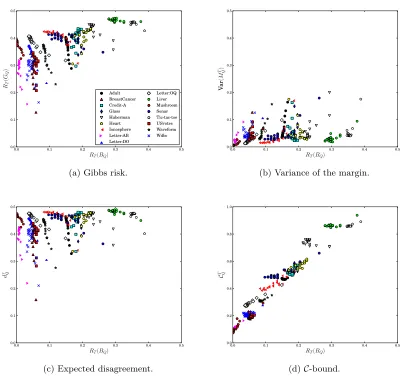
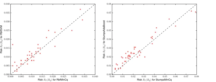
To further motivate the use of the C-bound, we investigate how its empirical value relates to the risk of the majority vote by conducting two experiments. The first experiment shows that the C-bound clearly outperforms the individual capacity of the other quantities of Theorem 11 in the task of predicting the risk of the majority vote. The second experiment shows that the C-bound is a great stopping criterion for Boosting algorithms.
4.5.1 Comparison with Other Indicators
We study howRD0(GQ), Var(MD
0
Q),dD
0
Q andCD
0
Q are respectively related toRD0(BQ). Note
that these four quantities appear in the first form or the third form of theC-bound (Theo-rem 11). We omit here the momentsµ1(MD
0
Q ) andµ2(MD
0
Q ) required by the second form of
theC-bound, as there is a linear relation betweenµ1(MD0
Q ) andRD0(GQ), as well as between µ2(MD
0
Q ) anddD
0
Q.
The results of Figure 3 are obtained with the AdaBoost algorithm of Schapire and Singer (1999), used with “decision stumps” as weak learners, on several UCI binary classification data sets (Blake and Merz, 1998). Each data set is split into two halves: a training set S
and a testing set T. We run AdaBoost on setS for 100 rounds and compute the quantities
RT(GQ), Var(MQT), dQT and CQT on set T at every 5 rounds of boosting. That is, we study
20 different majority vote classifiers per data set.
In Figure 3a, we see that we almost always haveRT(BQ)< RT(GQ). There is, however,
no clear correlation betweenRT(BQ) andRT(GQ). We also see no clear correlation between
RT(BQ) and Var(MQT) or betweenRT(BQ) anddQT in Figures 3b and 3c respectively, except
that generally RT(BQ) > Var(MQT) and RT(BQ) < dQT. In contrast, Figure 3d shows a
strong correlation betweenCQT andRT(BQ). Indeed, it is almost a linear relation! Therefore,
theC-bound seems well-suited to characterize the behavior of the Bayes risk, whereas each of the individual quantities contained in the C-bound is insufficient to do so.
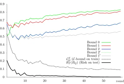
4.5.2 The C-bound as a Stopping Criterion for Boosting
0.0 0.1 0.2 0.3 0.4 0.5 RT(BQ)
0.0 0.1 0.2 0.3 0.4 0.5
RT
(
GQ
)
Adult BreastCancer Credit-A Glass Haberman Heart Ionosphere Letter:AB Letter:DO
Letter:OQ Liver Mushroom Sonar Tic-tac-toe USvotes Waveform Wdbc
(a) Gibbs risk.
0.0 0.1 0.2 0.3 0.4 0.5 RT(BQ)
0.0 0.1 0.2 0.3 0.4 0.5
Va
r
(
M
T Q)
(b) Variance of the margin.
0.0 0.1 0.2 0.3 0.4 0.5 RT(BQ)
0.0 0.1 0.2 0.3 0.4 0.5
d
TQ
(c) Expected disagreement.
0.0 0.1 0.2 0.3 0.4 0.5 RT(BQ)
0.0 0.2 0.4 0.6 0.8 1.0
C
T Q
(d)C-bound.
Figure 3: RT(BQ) versusRT(GQ), Var(MQT),dQT and CQT respectively.
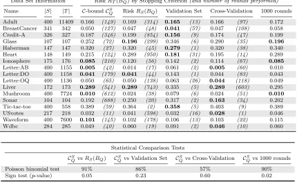
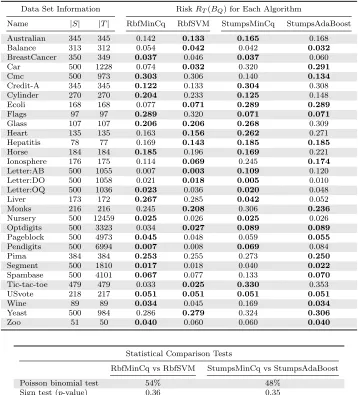
We use the same version of the algorithm and the same data sets as in the previous experiment. However, for this experiment, each data set is split into a training set S of at most 400 examples and a testing set T containing the remaining examples. We run AdaBoost on set S for 1000 rounds. At each round, we compute the empirical C-bound
CQS (on the training set). Afterwards, we select the majority vote classifier with the lowest
value ofCS
Qand compute its Bayes riskRT(BQ) (on the test set). We compare this stopping
criterion with three other methods. For the first method, we compute the empirical Bayes riskRS(BQ) at each round of boosting and, after that, we select the one having the lowest
such risk.7 The second method consists in performing 5-fold cross-validation and selecting the number of boosting rounds having the lowest cross-validation risk. Finally, the third method is to reserve 10% of S as a validation set, train AdaBoost on the remaining 90%,
Data Set Information RiskRT(BQ) by Stopping Criterion(and number of rounds performed) Name |S| |T| C-boundCS
Q RiskRS(BQ) Validation Set Cross-Validation 1000 rounds Adult 400 11409 0.166 (149) 0.169 (314) 0.165 (13) 0.166 (97) 0.172 BreastCancer 341 342 0.050 (127) 0.047 (48) 0.041 (57) 0.047 (108) 0.058 Credit-A 326 327 0.187 (346) 0.199 (854) 0.156 (9) 0.174 (47) 0.199 Glass 107 107 0.252 (72) 0.196 (299) 0.346 (6) 0.290 (35) 0.196 Haberman 147 147 0.320 (27) 0.320 (45) 0.279 (1) 0.320 (38) 0.340 Heart 148 149 0.215 (124) 0.289 (950) 0.181 (31) 0.195 (14) 0.289 Ionosphere 175 176 0.085 (210) 0.120 (56) 0.142 (2) 0.114 (67) 0.085 Letter:AB 400 1155 0.005 (42) 0.014 (17) 0.061 (2) 0.005 (60) 0.010 Letter:DO 400 1158 0.041 (179) 0.041 (44) 0.143 (1) 0.044 (83) 0.043 Letter:OQ 400 1136 0.050 (65) 0.050 (138) 0.063 (26) 0.044 (118) 0.049 Liver 172 173 0.289 (541) 0.289 (743) 0.335 (5) 0.289 (603) 0.295 Mushroom 400 7724 0.010 (612) 0.024 (38) 0.079 (6) 0.024 (51) 0.010 Sonar 104 104 0.192 (688) 0.250 (20) 0.317 (2) 0.163 (34) 0.202 Tic-tac-toe 400 558 0.389 (59) 0.364 (2) 0.358 (5) 0.403 (9) 0.389 USvotes 217 218 0.032 (11) 0.041 (598) 0.032 (16) 0.028 (1) 0.046 Waveform 400 7600 0.101 (145) 0.102 (178) 0.106 (13) 0.103 (22) 0.115 Wdbc 284 285 0.049 (40) 0.060 (19) 0.091 (2) 0.046 (10) 0.060
Statistical Comparison Tests
CS
QvsRS(BQ) CQS vs Validation Set C S
Qvs Cross-Validation C S
Qvs 1000 rounds
Poisson binomial test 91% 86% 57% 90%
Sign test (p-value) 0.05 0.23 0.60 0.02
Table 1: Comparison of various stopping criteria over 1000 rounds of boosting. The Poisson binomial test gives the probability thatCQS is a better stopping criterion than every other approach. The sign test gives ap-value representing the probability that the null hypothesis is true (i.e., the CQS stopping criterion has the same performance as every other approach).
and keep the majority vote with the lowest Bayes risk on the validation set. Note that this last method differs from the others because AdaBoost sees 10% fewer examples during the learning process, but this is the price to pay for using a validation set.
Table 1 compares the Bayes risks on the test setRT(BQ) of the majority vote classifiers
5. A PAC-Bayesian Story: From Zero to a PAC-Bayesian C-bound
In this section, we present a PAC-Bayesian theory that allows one to estimate theC-bound value CD
Q from its empirical estimate CQS. From there, we derive bounds on the risk of
the majority vote RD(BQ) based on empirical observations. We first recall the classical
PAC-Bayesian bound (here called the PAC-Bound 0) that bounds the true Gibbs risk by its empirical counterpart. We then present two different PAC-Bayesian bounds on the majority vote classifier (respectively called PAC-Bounds 1 and 2). A third bound, PAC-Bound 3, will be presented in Section 6. This analysis intends to be self-contained, and can act as an introduction to PAC-Bayesian theory.8
The first PAC-Bayesian theorem was proposed by McAllester (1999). Given a set of voters H, a prior distribution P on H chosen before observing the data, and a posterior distributionQon Hchosen after observing a training setS∼Dm (Qis typically chosen by running a learning algorithm onS), PAC-Bayesian theorems give tight risk bounds for the Gibbs classifierGQ. These bounds on RD(GQ) usually rely on two quantities:
a) The empirical Gibbs riskRS(GQ), that is computed on the mexamples of S,
RS(GQ) =
1
m
m
X
i=1 E
f∼QL`(f(xi), yi).
b) The Kullback-Leibler divergence between distributionsQandP, that measures “how far” the chosen posteriorQ is from the priorP,
KL(QkP) def= E
f∼Q ln
Q(f)
P(f). (20)
Note that the obtained PAC-Bayesian bounds are uniformly valid for all possible posteri-ors Q.
In the following, we present a very general PAC-Bayesian theorem (Section 5.1), and we specialize it to obtain a bound on the Gibbs risk RD(GQ) that is converted in a bound on
the risk of the majority voteRD(BQ) by the factor 2 of Proposition 10 (Section 5.2). Then,
we define new losses that rely on a pair of voters (Section 5.3). These new losses allow us to extend the PAC-Bayesian theory to directly bound RD(BQ) through the C-bound
(Sections 5.4 and 5.5). For each proposed bound, we explain the algorithmic procedure required to compute its value.
5.1 General PAC-Bayesian Theory for Real-Valued Losses
A key step of most PAC-Bayesian proofs is summarized by the followingChange of measure inequality (Lemma 17).
We present here the same proof as in Seldin and Tishby (2010) and McAllester (2013). Note that the same result is derived from Fenchel’s inequality in Banerjee (2006) and Donsker-Varadhan’s variational formula for relative entropy in Seldin et al. (2012); Tol-stikhin and Seldin (2013).
Lemma 17 (Change of measure inequality) For any set H, for any distributions P
and Q onH, and for any measurable function φ:H →R, we have
E
f∼Q φ(f) ≤ KL(QkP) + ln
E
f∼P e φ(f)
.
Proof The result is obtained by simple calculations, exploiting the definition of the KL-divergence given by Equation (20), and then Jensen’s inequality (Lemma 47, in Appendix A) on concave function ln(·) :
E
f∼Q φ(f) = fE∼Q lne
φ(f) = E
f∼Q ln
Q(f)
P(f) ·
P(f)
Q(f) ·e
φ(f)
= KL(QkP) + E
f∼Q ln
P(f)
Q(f) ·e
φ(f)
≤ KL(QkP) + ln
E
f∼Q
P(f)
Q(f) ·e
φ(f)
(Jensen’s inequality)
≤ KL(QkP) + ln
E
f∼P e φ(f)
.
Note that the last inequality becomes an equality ifQ andP share the same support.
Let us now present a general PAC-Bayesian theorem which bounds the expectation of any real-valued loss functionL:Y × Y →[0,1]. This theorem is slightly more general than the PAC-Bayesian theorem of Germain et al. (2009, Theorem 2.1), that is specialized to the expected linear loss, and therefore gives rise to a bound of the “generalized” Gibbs risk of Definition 5. A similar result is presented in Tolstikhin and Seldin (2013, Lemma 1).
Theorem 18 (General PAC-Bayesian theorem for real-valued losses) For any dis-tributionD on X × Y, for any setH of voters X → Y, for any loss L:Y × Y →[0,1], for any prior distribution P on H, for any δ ∈(0,1], for any m0 > 0, and for any convex functionD: [0,1]×[0,1]→R, we have
Pr S∼Dm
For all posteriorsQonH: D( E
f∼QE
L
S(f),fE
∼QE
L
D(f))≤ 1
m0
KL(QkP)+ln 1
δS∼EDmfE∼Pe
m0·D(ELS(f),E
L
D(f))
≥1−δ ,
where KL(QkP) is the Kullback-Leibler divergence between Qand P of Equation (20).
Most of the time, this theorem is used withm0 =m, the size of the training set. However, as pointed out by Lever et al. (2010), m0 does not have to be so. One can easily show
that different values of m0 affect the relative weighting between the terms KL(QkP) and ln 1δES∼DmEf∼Pem
0·D( ELS(f),E
L
D(f)) in the bound. Hence, especially in situations where these two terms have very different values, a “good” choice for the value ofm0 can tighten the bound.
Proof Note that E
f∼P e m0·D(
ELS(f),E
L
D(f)) is a non-negative random variable. By Markov’s inequality (Lemma 46, in Appendix A), we have
Pr
S∼Dm
E
f∼P e m0·D(
ELS(f),E
L
D(f)) ≤ 1
δS∼EDm fE∼P e
m0·D( ELS(f),E
L
D(f))
Hence, by taking the logarithm on each side of the innermost inequality, we obtain
Pr
S∼Dm
ln
E
f∼P e m0·D(
ELS(f),E
L
D(f))
≤ ln
1
δS∼EDm fE∼P e
m0·D( ELS(f),E
L
D(f))
≥1−δ .
We apply the change of measure inequality (Lemma 17) on the left side of innermost in-equality, with φ(f) =m0· D(ESL(f),ELD(f)). We then use Jensen’s inequality (Lemma 47,
in Appendix A), exploiting the convexity ofD :
∀Q onH: ln
E
f∼P e m0·D(
ELS(f),E
L
D(f))
≥ m0· E
f∼Q D(E L
S(f),ELD(f))−KL(QkP)
≥ m0· D( E
f∼QE L S(f), E
f∼QE L
D(f))−KL(QkP).
We therefore have
Pr S∼Dm
For all posteriorsQ:
m0
· D( E
f∼QE
L
S(f),fE
∼QE
L
D(f))−KL(QkP)≤ln
1
δS∼EDm fE∼P e
m0·D(ELS(f),E
L
D(f))
≥1−δ .
The result then follows from easy calculations.
As shown in Germain et al. (2009), the general PAC-Bayesian theorem can be used to recover many common variants of the PAC-Bayesian theorem, simply by selecting a well-suited functionD. Among these, we obtain a similar bound as the one proposed by Langford and Seeger (2001); Seeger (2002); Langford (2005) by using the Kullback-Leibler divergence between the Bernoulli distributions with probability of successqand probability of successp:
kl qkp) def= qlnq
p + (1−q) ln
1−q
1−p. (21)
Note that kl qkp) is a shorthand notation for KL(QkP) of Equation (20), withQ= (q,1−q) andP = (p,1−p). Corollary 50 (in Appendix A) shows that kl qkp) is a convex function.
In order to apply Theorem 18 withD(q, p) = kl(qkp) andm0 =m, we need the next lemma.
Lemma 19 For any distribution D on X × Y, for any voter f : X → Y, for any loss
L:Y ×Y →[0,1], and any positive integer m, we have
E
S∼Dm exp
m·klELS(f)kELD(f)
≤ ξ(m),
where
ξ(m) def=
m
X
k=0
m
k k m
k
1− k
m m−k
. (22)
Moreover, √m ≤ ξ(m) ≤ 2√m.
Proof Let us introduce a random variable Xf that follows a binomial distribution of m
As em·kl · kELD(f)
is a convex function, Lemma 51 (due to Maurer, 2004, and provided in Appendix A), shows that
E
S∼Dm exp
m·klELS(f)kELD(f)
≤ E
Xf∼B(m,ELD(f)) exp
m·klm1XfkELD(f)
.
We then have
E
Xf∼B(m,ELD(f))
emkl(m1XfkE
L
D(f))
= E
Xf∼B(m,ELD(f)) 1
mXf ELD(f)
!Xf
1− 1
mXf
1−ELD(f)
!m−Xf
=
m
X
k=0
Pr
Xf∼B(m,ELD(f))
Xf =k
·
k m ELD(f)
!k
1−mk 1−ELD(f)
!m−k
= m X k=0 m k
ELD(f)
k
1−ELD(f)
m−k ·
k m ELD(f)
!k
1− mk 1−ELD(f)
!m−k
= m X k=0 m k k m k
1− k
m m−k
= ξ(m).
Maurer (2004) shows that ξ(m) ≤2√m form ≥8, and ξ(m) ≥√m form ≥2. However, the cases form∈ {1,2,3,4,5,6,7}are easy to verify computationally.
Theorem 20 below specializes the general PAC-Bayesian theorem toD(q, p) = kl(qkp), but still applies to any real-valued loss functions. This theorem can be seen as an intermediate step to obtain Corollary 21 of the next section, which uses the linear loss to bound the Gibbs risk. However, Theorem 20 below is reused afterwards in Section 5.3 to derive PAC-Bayesian theorems for other loss functions.
Theorem 20 For any distribution D on X ×Y, for any set H of voters X → Y, for any loss L:Y × Y →[0,1], for any prior distribution P on H, for anyδ ∈(0,1], we have
Pr
S∼Dm
For all posteriors Q onH:
kl
E
f∼QE L S(f)
E
f∼QE L D(f)
≤ 1
m
KL(QkP) + lnξ(m)
δ
≥ 1−δ .
Proof By Theorem 18, with D(q, p) = kl(qkp) andm0=m, we have
Pr S∼Dm
∀QonH: kl( E
f∼QE
L
S(f)kfE
∼QE
L
D(f))≤ 1
m
KL(QkP)+ln 1
δS∼EDmfE∼Pe
m·kl(ELS(f)kE
L
D(f))
≥1−δ .
As the priorP is independent ofS, we can swap the two expectations in E
S∼DmfE∼Pe
m·kl(·k·). This observation, together with Lemma 19, gives
E
S∼Dm fE∼Pe
m·kl(ELS(f)kE
L
D(f)) = E
f∼P S∼EDme
m·kl(ELS(f)kE
L
D(f)) ≤ E
5.2 PAC-Bayesian Theory for the Gibbs Classifier
This section presents two classical PAC-Bayesian results that bound the risk of the Gibbs classifier. One of these bounds is used to express a first PAC-Bayesian bound on the risk of the majority vote classifier. Then, we explain how to compute the empirical value of this bound by a root-finding method.
5.2.1 PAC-Bayesian Theorems for the Gibbs Risk
We interpret the two following results as straightforward corollaries of Theorem 20. Indeed, from Definition 5, the expected linear loss of a Gibbs classifier GQ on a distribution D0 is
RD0(GQ). These two Corollaries are very similar to well-known PAC-Bayesian theorems. At
first, Corollary 21 is similar to the PAC-Bayesian theorem of Langford and Seeger (2001); Seeger (2002); Langford (2005), with the exception that lnm+1δ is replaced by lnξ(mδ). Since
ξ(m) ≤ 2√m ≤ m+ 1, this result gives slightly better bounds. Similarly, Corollary 22 provides a slight improvement of the PAC-Bayesian bound of McAllester (1999, 2003a).
Corollary 21 (Langford and Seeger, 2001; Seeger, 2002; Langford, 2005) For any distri-bution D onX ×{−1,1}, for any set H of voters X →[−1,1], for any prior distributionP
onH, and any δ ∈(0,1], we have
Pr
S∼Dm
For all posteriors Q onH: kl RS(GQ)
RD(GQ)
≤ 1
m
KL(QkP) + lnξ(m)
δ
≥ 1−δ .
Proof The result is directly obtained from Theorem 20 using the linear loss L = L` to
recover the Gibbs risk of Definition 5.
Corollary 22 (McAllester, 1999, 2003a) For any distribution D on X ×{−1,1}, for any setHof voters X →[−1,1], for any prior distributionP onH, and anyδ ∈(0,1], we have
Pr
S∼Dm
For all posteriors Q onH:
RD(GQ) ≤ RS(GQ) +
s
1 2m
KL(QkP) + lnξ(m)
δ
≥ 1−δ .
Proof The result is obtained from Corollary 21 together with Pinsker’s inequality 2(q−p)2 ≤ kl(qkp).
We then have
Pr S∼Dm
For all posteriorsQonH:
2·RS(GQ)−RD(GQ) 2
≤ m1
KL(QkP) + lnξ(m)
δ
≥ 1−δ .
The result is obtained by isolating RD(GQ) in the inequality, omitting the lower bound of
RD(GQ). Recall that the probability is “≥1−δ”, hence if we omit an event, the probability
5.2.2 A First Bound for the Risk of the Majority Vote
Let assume that the Gibbs risk RD(GQ) of a classifier is lower than or equal to 12. Given
an empirical Gibbs riskRS(GQ) computed on a training set ofm examples, the
Kullback-Leibler divergence KL(QkP), and a confidence parameter δ, Corollary 21 says that the Gibbs riskRD(GQ) is included (with confidence 1−δ) in the continuous setRQ,Sδ defined as
RQ,Sδ
def =
r : kl RS(GQ)
r
≤ 1
m h
KL(QkP) + lnξ(m)
δ i
and r≤ 1 2
. (23)
Thus, an upper bound onRD(GQ) is obtained by seeking the maximum value ofRQ,Sδ . As
explained by Proposition 10, we need to multiply the obtained value by a factor 2 to have an upper bound on RD(BQ). This methodology is summarized by PAC-Bound 0.
Note that PAC-Bound 0 is also valid when RD(GQ) is greater than 12, because in this
case, 2 ·supRQ,Sδ = 1 (with confidence at least 1−δ), which is a trivial upper bound of RD(BQ).
PAC-Bound 0 For any distributionDonX ×{−1,1}, for any setHof votersX →[−1,1], for any prior distribution P on H, and any δ∈(0,1], we have
Pr
S∼Dm
∀Q onH : RD(BQ) ≤ 2·supRQ,Sδ
≥ 1−δ .
Proof If supRQ,Sδ = 12, the bound is trivially valid because RD(BQ) ≤1. Otherwise, the
bound is a direct consequence of Proposition 10 and Corollary 21.
As we see, the proposed bound cannot be obtained by a closed-form expression. Thus, we need to use a strategy as the one suggested in the following.
5.2.3 Computation of PAC-Bound 0
One can compute the valuer= supRQ,Sδ of PAC-Bound 0 by solving
kl RS(GQ)
r
= m1KL(QkP) + lnξ(mδ), withRS(GQ)≤r≤ 12,
by a root-finding method. This turns out to be an easy task since the left-hand side of the equality is a convex function of r and the right-hand side is a constant value. Note that solving the same equation with the constraint r ≤ RS(GQ) gives a lower bound of
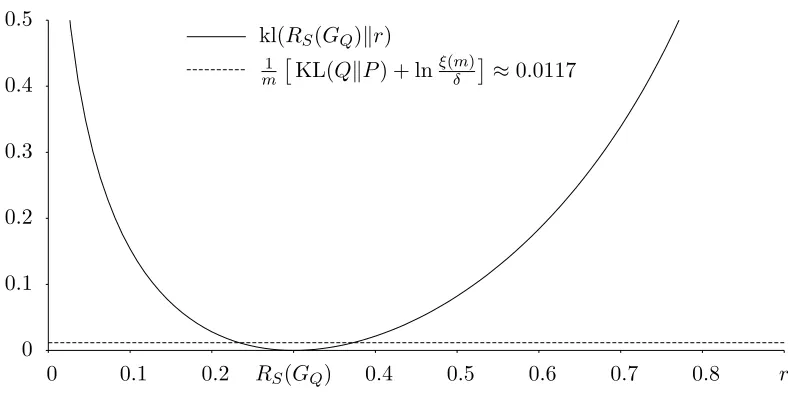
RD(GQ), but not a lower bound on RD(BQ). Figure 4 shows an application example of
PAC-Bound 0.
5.3 Joint Error, Joint Success, and Paired-voters
0 0.1 0.2 0.3 0.4 0.5
0 0.1 0.2 RS(GQ) 0.4 0.5 0.6 0.7 0.8 r
kl(RS(GQ)kr)
1
m
KL(QkP) + lnξ(mδ)
≈0.0117
Figure 4: Example of application of PAC-Bound 0. We suppose that KL(QkP) = 5, m= 1000 and δ = 0.05. If we observe an empirical Gibbs risk RS(GQ) = 0.30, then
RD(GQ) ∈ RQ,Sδ ≈ [0.233,0.373] with a confidence of 95%. On the figure, the
intersections between the two curves correspond to the limits of the intervalRQ,Sδ . Then, with these values, PAC-bound 0 givesRD(BQ).2·0.373 = 0.746.
5.3.1 The Joint Error and the Joint Success
We have already defined the expected disagreementdD0
Q of a distributionQof voters
(Defi-nition 7). In the case of binary voters, the expected disagreement corresponds to
dD0
Q = hE
1∼Q
E
h2∼Q
E
(x,y)∼D0 I(h1(x)6=h2(x))
.
Let us now define two closely related notions, the expected joint successsD0
Q and the expected
joint erroreD0
Q. In the case of binary voters, these two concepts are expressed naturally by
eD0
Q = h1∼EQ h2∼EQ
E
(x,y)∼D0 I(h1(x)=6 y)I(h2(x)6=y)
,
sD0
Q = hE
1∼Q
E
h2∼Q
E
(x,y)∼D0 I(h1(x) =y)I(h2(x) =y)
.
Let us now extend in the usual way these equations to the case of real-valued voters.
Definition 23 For any probability distributionQon a set of voters, we define theexpected joint error eD0
Q relative toD
0 and theexpected joint success sD0
Q relative toD 0 as
eD0
Q
def
= E
f1∼Qf2E∼Q
E
(x,y)∼D0 L`(f1(x), y)· L`(f2(x), y)
,
sD0
Q
def
= E
f1∼Qf2E∼Q
E (x,y)∼D0
h
1− L`(f1(x), y)
i
·h1− L`(f2(x), y)
From the definitions of the linear loss (Definition 2) and the margin (Definition 8), we can easily see that
eD0
Q = (x,yE)∼D0
1−MQ(x, y)
2
2
= 1 4
1−2·µ1(MD
0
Q ) +µ2(MD
0
Q )
,
sD0
Q = (x,yE)∼D0
1 +MQ(x, y)
2
2
= 1 4
1 + 2·µ1(MD
0
Q ) +µ2(MD
0
Q )
.
Remembering from Equation (9) that dD0
Q = 12
1−µ2(MD0
Q )
, we can conclude that eD0
Q,
sD0
Q and dD
0
Q always sum to one:9
eD0
Q + sD
0
Q + dD
0
Q = 1.
We can now rewrite the first moment of the margin and the Gibbs risk as
µ1(MD
0
Q ) = sD
0
Q −eD
0
Q = 1−(2eD
0
Q +dD
0
Q),
RD0(GQ) = 1
2(1−s D0
Q +eD
0
Q) = 12(2e D0
Q +dD
0
Q). (24)
Therefore, the third form ofC-bound of Theorem 11 can be rewritten as
CDQ0 = 1−
1−(2eD0
Q +dD
0
Q)
2
1−2dD0
Q
. (25)
5.3.2 Paired-Voters and Their Losses
This first generalization of the PAC-Bayesian theorem allows us to boundseparately either
dD
Q, eDQ or sDQ, and therefore to bound CQD. To prove this result, we need to define a new
kind of voter that we call a paired-voter.
Definition 24 Given two voters fi : X → [−1,1] and fj : X → [−1,1], the paired-voter
fij :X →[−1,1]2 outputs a tuple:
fij(x) def= hfi(x), fj(x)i.
Given a set of votersHweighted by a distributionQonH, we define a set of paired-votersH2 weighted by a distribution Q2 as
H2 def= {f
ij : fi, fj ∈ H}, and Q2(fij) def= Q(fi)·Q(fj). (26)
We now present three losses for paired-voters. Remember that a loss function has the form Y ×Y → [0,1], where Y is the voter’s output space. As a paired-voter output is a
tuple, our new loss functions map [−1,1]2× {−1,1} to [0,1]. Thus,
Le fij(x), y
def
= L`(fi(x), y)· L`(fj(x), y),
Ls fij(x), y
def
=
h
1− L`(fi(x), y)
i
·h1− L`(fj(x), y)
i ,
Ld fij(x), y
def
= L`(fi(x)·fj(x),1). (27)
The key observation to understand the next theorems is that the expected losses of paired-voters H2 defined by Equation (26) allow one to recover the values of eD0
Q,sD
0
Q and
dD0
Q. Indeed, it directly follows from Definitions 3, 7 and 23, that
eD0
Q = E
fij∼Q2
ELDe0
fij
; sD0
Q = E
fij∼Q2
ELDs0
fij
; dD0
Q = E
fij∼Q2
ELDd0
fij
. (28)
5.4 PAC-Bayesian Theory For Losses of Paired-voters
As explained in Section 5.2, classical PAC-Bayesian theorems, like Corollaries 21 and 22, provide an upper bound onRD(GQ) that holds uniformly for all posteriors Q. A bound on
RD(BQ) is typically obtained by multiplying the former bound by the usual factor of 2, as
in PAC-Bound 0.
In this subsection, we present a first bound of RD(BQ) relying on theC-bound of
Theo-rem 11. A uniform bound onCQD is obtained using the third form of theC-bound, through a bound on the Gibbs riskRD(GQ) and another bound on the disagreement dDQ. The desired
bound on RD(GQ) is obtained by Corollary 21 as in PAC-Bound 0. To obtain a bound
on dD
Q, we capitalize on the notion of paired-voters presented in the previous section. This
allows us to express two new PAC-Bayesian bounds on the risk of a majority vote, one for the supervised case and another for the semi-supervised case.
5.4.1 A PAC-Bayesian Theorem for eDQ, sDQ, or dDQ
The following PAC-Bayesian theorem can either bound the expected disagreementdD
Q, the
expected joint successsD
Qor the expected joint erroreDQof a majority vote (see Definitions 7
and 23).
Theorem 25 For any distributionD onX ×{−1,1}, for any set Hof voters X →[−1,1], for any prior distribution P on H, and any δ∈(0,1], we have
Pr
S∼Dm
For all posteriors Q on H:
kl αS
Q
αDQ
≤ 1
m
2·KL(QkP) + lnξ(m)
δ
≥ 1−δ ,
where αD0
Q can be either eD
0
Q,sD
0
Q or dD
0
Q.
Proof Theorem 25 is deduced from Theorem 20. We present here the proof forαD0
Q =eD
0
Q.
The two other cases are very similar.