Telephone: +44 (0)1582 763133 Web: http://www.rothamsted.ac.uk/
Rothamsted Repository Download
C2 - Non-edited contributions to conferences
Thompson, R. 2009. Latent mixed models. Proceedings 18th Conference
of the Association for the Advancement of Animal Breeding and Genetics:
Matching Genetics and the Environment - a New Look at an Old Topic,
Barossa Valley, 28 September - 1 October 2009 . Association for the
Advancement of Animal Breeding Genetics. pp. 398-405
The output can be accessed at:
https://repository.rothamsted.ac.uk/item/8q66w
.
© 28 September 2009, Association for the Advancement of Animal Breeding Genetics.
LATENT MIXED MODELS
Robin Thompson
Centre for Mathematical and Computational Biology, and Department of Biomathematics and Bioinformatics, Rothamsted Research, Harpenden AL5 2JQ, UK and School of Mathematical
Sciences, Queen Mary, University of London, Mile End Road, London E1 4NS, UK
SUMMARY
The linear mixed model has been a major research interest of Dr Arthur Gilmour, motivated by problems arising in research data generated by agricultural scientists. He has developed a variety of computer packages associated with the linear mixed model. He has tirelessly assisted researchers in the analysis and interpretation of their data using these packages. In this quest to help researchers he has made several important innovations. The purpose of this paper is to review some of these innovations, including improved iterative schemes for estimating variance parameters, developing a powerful scheme for specification of linear mixed models and exploiting sparsity to reduce the computational burden. Some of these innovations are only implicitly described in computer user guides and deserve wider recognition.
INTRODUCTION
In this paper we review some of the contributions of Dr Arthur Gilmour to the analysis of correlated data, especially that generated by agricultural scientists. He has developed several packages that help with this analysis including REG (Gilmour 1993a), a generalised linear model program, TwoD (Gilmour 1992), a program for the analysis of spatial data, BVEST (Gilmour 1993b), a program for the prediction of breeding values using best linear unbiased prediction (BLUP) and more recently ASReml (Gilmour et al. 2006) a program for the analysis of mixed models. In this paper some of the features involved in the development of this program will be reviewed, including some of the theory behind the program, the specification of the model and taking account of sparsity in various algorithms introduced to reduce the computational burden.
THEORY
Some of the main points arise by considering a linear model of the form
′ ′
′ ′
′ ′
(1)
where y is the vector of phenotypic measurements and X is the design matrix for fixed effects, τ,
Z is the design matrix for random effects, u, and e is the vector of model residuals and where effects vector, u, and the residual vector, e, are assumed to be multivariate normally distributed with varu . Because this linear model includes fixed effects, τ, and random effects, u,
this is called a mixed model. It has many applications. In the analysis of experiments interest is in estimation of treatment effects, , taking account of the correlated variance structure. In some genetic applications there is interest in estimation of the genetic variances and covariances in G, adjusting the data for the fixed effects . In other applications, which particularly motivated Henderson, there is interest in predicting the random effects u and Henderson (1973) introduced the system of equations
(2)
and showed that the solutions for the random effects are the Best Linear Unbiased Predictors (BLUPs) of those effects. Given R and G, the solution for the fixed effects given by these equations is the same as given by solving where ′. Because of the similarity of these equations to least squares equations, which are the same as (2) but without the term, these equations are now called Henderson’s mixed model equations.
′ ′
In other cases there is interest in parameterizing R and G, as a function of variance parameters and estimating these variance parameters. Patterson and Thompson (1971) introduced a residual maximum likelihood (REML) method based on maximising the likelihood of error contrasts i.e. contrasts that contributed no information on fixed effects. This REML method agreed with analysis of variance methods in balanced cases and effectively eliminated bias in variance estimation due to not knowing the fixed effects. Convenient forms of the residual log-likelihood (Harville 1974, Smith and Graser 1985) are
L=-(0.5)(D+S), where D=logdet(V)+logdet( ) = logdet(G)+logdet(R)+logdet(C) and , is a residual sum of squares with
with W=[X Z].
This residual likelihood is of the same form as the full likelihood with the addition of the last term in D that is sometimes thought of as a penalty for estimating the fixed effects. Smith and Graser (1985) introduced the form that is a function of C that naturally leads to sequential formation of the likelihood. The terms D and S can be formed sequentially by using terms associated with eliminating, or absorbing, the fixed and random effects one by one from the MME. An advantage of this is that C–1 is not calculated and, because of the large number of zero elements in C, computation can be substantially reduced by using sparse matrix methods. One disadvantage was that the differentials of the likelihood were not easily available. To maximize the likelihood with one parameter Smith and Graser (1985) suggested using a quadratic approximation. With more than one parameter, methods that avoid calculating derivatives become a popular flexible alternative, and the DFREML program written by Meyer (1991a) was used extensively. For example, these methods were used for Animal and Reduced Animal Models, both for univariate and multivariate data (Meyer, 1989, 1991b). The basic framework was extended to include more biologically appropriate models with genetic components, including maternal models with both Wilham and Falconer terms (Koerhuis and Thompson, 1997), and models with mutation terms (Wray, 1990).
the differential of the sum of squares S, and can be written in the similar way to S itself, using working variables based on estimates of the fixed effects and predictors of the random effects.
A synthesis of comparisons of different algorithms used to compute REML estimates was carried out by Hofer (1998) and is updated in Table 1. These comparisons show the expected improvement of EM methods over derivative free methods. The comparisons also show that most second differential methods converge in relatively few iterations.
Table 1. Results of empirical comparison of REML algorithms with regards to rounds of iteration (function evaluations for DF) and total time to convergence a
Refa MMEb Parc DFd EM NR/AIe F.Eval Time (h) Rounds Time (h) Rounds Time (h)
1 4895 3 26 0.01 24 0.05
9790 9 238 0.31 33 0.26
14685 18 583 1.77 45 1.02
2 6192 9 699 1.27 6 0.45
10230 12 1236 2.33 8 0.90
14274 18 4751 11.10 18 3.33
3 5731 5 169 0.34 6 0.07
4 8765 6 927 70.6 109 1.14 7 1.86
5 5073 2 39 0.02 23 4.97 5 0.02
6f 233796 55 37021 2083 185 40.10
7 46581 12 1435 15.2 1006 88.6 6 0.58
55410 19 5813 30.6 6 1.00
a
References 1 Misztal 1999; 2 Meyer and Smith 1996; 3 Johnson and Thompson 1995 ; 4 Gilmour et al. 1995; 5 Madsen et al. 1994 ; 6 Neumaier and Groeneveld 1998;
7 Jensen et al. 1997
b
Dimension of mixed model equations (MME).
c
Number of (co)variance components.
d
‘DF’ = derivative free
e
‘NR’ = quasi-Newton using computed analytic differences.
f
quasi -Newton using finite differences.
APPLICATION
With the availability of an efficient algorithm for the calculation of the sparse inverse of C and for the calculation of an AI matrix there was interest in developing a general program for estimating variance parameters. This program ,now called ASReml (Gilmour et al. 2006), was designed taking into account features in existing programs. These included REG (Gilmour 1993 )a program for estimation of generalized linear models, TwoD (Gilmour 1992), a program for spatial analysis, REML (Thompson 1977,Robinson et al. 1982), a program developed for the analysis of variety trials that had been ported to Genstat, (Welham and Thompson 1990) and DFEML (Meyer 1991a).
Linear model specification. The specification of the design matrices X and Z in (1) initially followed the Wilkinson and Rogers (1973) syntax that allowed interaction between factorial terms and the specification of polynomial and regression sub models associated with factorial terms. This specification of models was very general but several modifications were found to be of value to ease the setting up of the linear model terms.
Conditional factors. Sometimes effects are only required to be fitted for subsets of the data. The at() function allows this. For example at(HERD.1).SEASON allows SEASON effects just for data with HERD =1. If no levels of the conditioning factor (at(HERD).SEASON in this case) are specified in the at() function, a complete set of conditioning terms is generate and this allows estimation of variance models for SEASON effects for each level of HERD.
Combining design matrices. There is sometimes the need to combine or overlay design matrices. The and() function allows this. For example SIREBREED and(DAMBREED) allows models with equal SIREBREED and DAMBREED effects to be fitted and this might be useful in the analysis of diallel crosses .Sometimes there is the need to associate competition effects from animals in the same group(Bijma et al.,2006). For example if there are 4 animals in each group and DIRECT is a factor indicating each animal and INDIRECT1, INDIRECT2, INDIRECT3 are factors indicating the 3 animals in the same group this can again be modelled using DIRECT and(INDIRECT1) and(INDIRECT2) and(INDIRECT3).
Functions of covariates and factorial effects. ASReml originally allowed model terms that were polynomials of covariates but there is sometimes interest in forming other functions ,for example when fitting splines. To add generality the facility to form user generated functions was added .For example, if the values of a covariate c are then reading in a file with i-th row
with i=1,…,L and j=1,…,L* and allows the functions with j=1,…,L* to be constructed and used in a model. Similarly if the effects, , for a factor with L levels are required to be replaced by , for example if some elements of are constrained, then again the ,possibly non-zero, elements of the L matrix F can be read in and the effects incorporated into the linear model.
, … ,
Variance specification. In the simplest case when the random effects were all uncorrelated allowed easy specification of the variance structure of the model. However the programs REML and TwoD and the need of users for various models including seperable spatial processes, random regression models and multivariate animal models inspired a wider class of models. Firstly both R
and G were allowed to be expressed as a direct sum of respectively s and b parts i.e.
and
and
and
The effects associated with each part are uncorrelated with effects in the other parts. This generality of R was partly to allow the analysis of a series of trials with possibly different numbers of plots and different variance parameters in each trial. The parameter b relates to the number of sets of random effects embedded in the random effects u. Models for the component matrices
are allowed to be formed as the direct product of models for up to three correlated
random factorsof the form .
A range of models are available for the components of both R and G, They include correlation models and covariance models. Correlation models generate variance matrices, C , with diagonals one, include uniform, banded and general correlation and models motivated by time-series analysis including autoregressive, moving average and autoregressive-moving average models. The covariance models, generate a variance matrix V, include diagonal, ante dependence, unstructured and factor analytic models. There is also the facility to form homogeneous variance matrices
correlation matrix C, the scalar and the parameters in the diagonal matrix (Gilmour et al. 1998). There is also the facility to form an additive relationship matrix from a pedigree, and fit cubic splines by incorporating an equivalent mixed model (Verbyla et al., 1999).Typically a variance structure applies to individual terms in the linear model but the facility is available to impose structure on a combination of terms, for example if there are effects ANIMAL and ANIMAL.TIME with ANIMAL representing animal effects and TIME a covariate and wish to impose random animal terms and animal regression terms and a covariance between these two sets of terms.
/
then if
. .
.
Despite the generality of the variance models one cannot always predict the ingenuity of users (for example Jaffervic et al. 2004)and so there is the facility to read in a user generated relationship matrix or its inverse and there is a facility to allow users to define variance matrices (or their inverses) as functions of parameters to be estimated. One problem with user generated relationship matrices is that they may, perhaps due to sampling, be singular. For example a relationship matrix
A may have rank r and have s singularities, then if we reorder A so that A and the associated
random effects can be partitioned as and with of rank r
then because of the s singularities . and the random effects are given by . One might extend using
with the same size as and setup MME using and
replacing u and in (2).Note that if is positive definite then with absorption of the mixed model equations reduce to the usual form. If , can be thought ofas introducing Lagrange multipliers to take account of the constraints on .
Exploiting sparsity. The MME and the inverse variance matrices involved in the MME are typically sparse with a large number of zero elements. Some of the computational work can be reduced if due account of this sparsity is taken. This reduction includes calculation of the likelihood and its differentials, calculation of variances of linear functions of the effects, and calculations involved with factor analysis models.
Calculation of the likelihood and its differentials. This involves the sequential calculation of the weighted sum of squares, S, and the calculation of the sparse inverse of Cdepend on the order that the order of terms in C. For example in a simple example with model with a grand mean and h uncorrelated herd effects, then C has h+1 rows and columns and 1+3h non-zero elements in C.If the sequential formation starts by eliminating the grand mean the resulting updated C matrix fills in the non-zero elements of C and the sparse inverse requires calculation of all elements of C–1.By contrast, if in the sequential formation the grand mean is the last term then there is no in-fill of C
and only the 1+3h elements, corresponding to the non-zero elements in the initial C, need calculating in the sparse inverse of C. The computation time with the initial ordering is proportional to and proportional to h in the later scheme.
(iii) absorb rows shorter than the cut-off at the time they are considered for absorption, starting with the shortest row. Once all rows with non-zero elements less than the cut-off have been absorbed then the program goes back to step (i) and the process is repeated until all the rows have been absorbed.
After experimentation an extra grouping step was introduced giving a grouped nested search algorithm(GNS).This grouping step identifies rows which have the same columns present. Each such group of rows is represented by just one member in the list of equations yet to be absorbed; the whole group is absorbed when that representative is absorbed. This has little impact on the order obtained but does reduce the work required to determine the order.
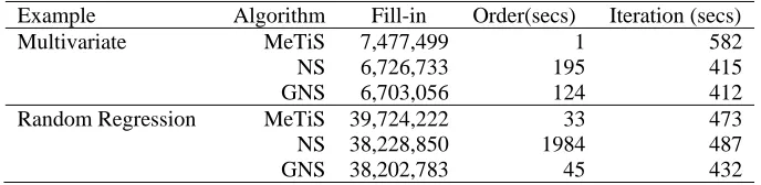
Timings for two examples are given in Table 2 for these two ordering algorithms (NS and GNS) and another suggested ordering (MeTiS). Ducrocq and Druet (2003) identified the MeTiS suite of ordering algorithms (Karypis and Kumar, 1998) as being very suitable for the solution of
Table 2. Fill-in(size of coefficient matrix after absorption) and timing for ordering and one iteration for two examples and three algorithms run on a 32bit Linux.
Example Algorithm Fill-in Order(secs) Iteration (secs)
Multivariate MeTiS 7,477,499 1 582
NS 6,726,733 195 415
GNS 6,703,056 124 412
Random Regression MeTiS 39,724,222 33 473
NS 38,228,850 1984 487
GNS 38,202,783 45 432
mixed model equations. These algorithms are based on a multilevel k-way partitioning of graphs. MeTiS uses initial coarsening, partitioning and then uncoarsening resulting in multilevel, nested dissection involving top-down and bottom-up ordering. Meyer (2005) evaluated MeTiS in her software, comparing it to a range of other published algorithms including the multiple minimum degree routine GENMMD (George and Liu, 1981, Lui, 1985) and various refinements extracted from the MUMPS package (Amestoy et al., 1998, 2001). She concluded MeTiS produced orderings which required about half the execution time of the minimum degree algorithms although the times vary a little with the particular characteristics of the example.
The first example is a six trait multivariate sire model analysis of data from 26875 animals fitting 31745 equations and 39 variance parameters. The second example is a multivariate random regression of 437,632 data records fitting 536,288 equations and 116 variance parameters. The MeTiS ordering routines quickly find a good order for solving mixed model equations. However, in the context of ASReml, the MeTiS order is on balance not the optimum order when compared with the GNS ordering algorithm. This is often 10-20% faster per iteration.
Calculation of variances of linear functions of the effects. It sometimes required to estimate a linear combination of the fixed and random effects and with the variance of this combination is . By replacing the right hand side of equation (3) by it can be shown (Gilmour et al. 2004) that the variance of the linear combination could be found in a sparse way in exactly same way as the fitted sum of squares from the linear model (1).
as , , and of size , and respectively.
can be then be written as ′
′ with var
and
may represent the performance of the i-th genotype in p environments or p different traits.This is motivated by writing the elements of as linear combinations of the k elements of and the first r of the elements of having extra components based on .The variance matrix of
′ ′
.If r=0 then we have
a reduced rank model (Meyer2005). If are usedinstead of using ,in the mixed model equations then the sparsity increases especially if k is much less than p because the inverse matrix associated with these terms is sparser than the inverse variance matrix associated with . Thompson et al. (2003) give examples where the alternative parameterization had savings of 50% of computational time when p=3 and k=3 and savings of 90% when p=62 and k=3.
Also if the effects are associated with genotype i, and are combined into a vector u , and the genotypes have an additive relationship matrix A then var(u)= . The calculation of the average information matrix requires the calculation of terms such as s=Ar where r is a vector of residuals (Kelly et al. 2009). As is much sparser than A, Kelly et al . (2009) found it useful to think ofsas the solution to s=r. This solution can be found in a recursive way first adjusting the right hand sides of ancestors for direct descendants and then adjusting direct descendents for ancestors (Kelly et al. 2009).This computation avoids the formation of A and the computational effort is linear in the number of genotypes.
DISCUSSION
The initial motivation in developing the computer program was to generate a kernel to be ported into Genstat. Such was the enthusiasm for the methods that a standalone program was developed, partly using code from REG to allow a wide range of data transformations. This has needed much more support but has the advantage that the algorithm has been made available to a wider user community. The user guide has been cited in over 1,000 publications. These publications are an appropriate testimony to the insight and innovations of Arthur Gilmour.
ACKNOWLEDGEMENTS
This research was supported by Lawes Agricultural Trust. I acknowledge the unstinting help Arthur Gilmour has given me over my career.
REFERENCES
Amestoy, P.R., Duff, I.S. and Excellent, J.-Y. (1998) Comp. Methods Appl. Mech. Eng.184 :501 Amestoy, P.R., Duff, I.S., Koster, J. and Excellent, J.-Y. (2001) SIAM J. Matrix Anal. Appl.23 :15. Bijma,P., Muir, W.M., Ellen, E.D., Wolf, J.B. and Van Arendonk, J.A.M. (2007) Genetics 175:
289.
Ducrocq, V. and Druet, T. (2003) 54th Annual Meeting, Europ. Ass. Anim. Prod. :1.
Henderson, C.R. (1973) In “Proc. Animal Breeding and Genetics. Symposium in Honor of Dr. Jay L. Lush” Amer. Soc. of Anim. Sci. and Amer. Dairy Sci. Assoc., Champaign, Illinois, p. 10. George, A. and Liu, J. W.-H. (1981) Computer Solution of Large Positive Definite Systems. Prentice-Hall, Inc., Englewood Cliffs, New Jersey.
Gilmour, A.R. (1992) “TwoD. A program to fit a mixed linear model with two dimensional spatial adjustments for local trend” NSW Agriculture, Tamworth, Australia.
Gilmour, A.R. (1993a) “REG - A generalised linear models program” NSW Agriculture, Orange, Australia.
Gilmour, A.R., Cullis, B.R., Frensham, A.B. and Thompson, R. (1998). Compstat'98 Proceedings 53.
Gilmour, A.R., Cullis, B.C., Welham, S.J., Gogel, B.J. and Thompson, R (2004) Computational Statistics and Data Analysis 44:571.
Gilmour, A.R., Gogel, B., Cullis, B.R. and Thompson, R. (2006) “ASReml 2 User Guide” VSN International, Hemel Hempstead, UK.
Gilmour, A.R. and Thompson, R. (2006) 8th World Congr. Genet. Appl. Livest. Prod. 27:12. Gilmour, A.R., Thompson, R. and Cullis, B.R. (1995) Biometrics 51:1440.
Harville, D.A. (1974) Biometrika 61:383.
Hill, W.G. and Thompson, R. (1978) Biometrics 34: 429. Hofer, A. (1998). J. Anim. Breed. Genet. 115:247.
Jaffrézic, F. , White, I. M. S. , Thompson, R. , Hill, W. G. and Visscher, P. (2002) J. of Dairy Science 85:968.
Johnson, D.L. and Thompson, R (1995) J. Dairy Sci., 78:449.
Jensen, J., Mantysaari, E.A., Madsen, P. and Thompson, R. (1997) Indian Journal of Agric. Stat.
49: 215.
Karypis, G. and Kumar, V. (1998) SIAM Journal of Scientific Computing, 20: 359.
Kelly, A.M., Cullis, B.R., Gilmour, A.R., Eccleston, J.A. and Thompson, R. (2009) Genetics, Selection and Evolution 41:33.
Koerhuis, A.N.M. and Thompson, R. (1997). Genetics, Selection and Evolution 29:225. Liu, J. W.-H. (1985) ACM Trans. Mathh. Soft. 11 :141.
Madsen, P., Jensen, J. and Thompson, R. (1994) 5th World Congr. Genet. Appl. Livest. Prod.
22:19.
Meyer, K. (1989) Genetics, Selection and Evolution 21:317.
Meyer, K. (1991a) “DFREML User Notes Version 2.0” University of New England, Armidale, Australia.
Meyer, K. (1991b) Genetics, Selection and Evolution 23:67.
Meyer, K. and Smith, S.P. (1996). Genetics, Selection and Evolution 28:23. Meyer, K. (2005) Proc. Assoc. Advmt. Anim. Breed. Genet. 16: 282. Meyer, K. (2008) Genetics, Selection and Evolution 40:3.
Misztal, I. (1994) J. Anim. Breed. Genet. 111:346.
Misztal, I. and Perez-Enciso, M. (1993) J. Dairy Sci. 76:1479. Neumaier, A. and Groeneveld, E. (1998) Genet. Sel. Evol. 30: 3.
Robinson, D.L., Thompson, R. and Digby, P.G.N. 1982. COMPSTAT 1982, II, Physica-Verlag, Wien :231.
Patterson, H.D. and Thompson, R. (1971) Biometrika58:545. Thompson, R. (1977) Biometrics 33:497.
Thompson, R., Cullis, B.C., Smith, A. and Gilmour, A.R. (2003) Australian and New Zealand Journal of Statistics 45:445.
Smith, S.P. (1995) J. Comp. Graph Stat. 4:134.
Smith, S.P. and Graser, H.-U. (1986) J. Dairy Sci. 69:1156.
Takahashi, K., Fagan, J. and Chin, M.S. (1973). Proc. 8th Inst. PICA Conf., Minneapolis: 63. Verbyla, A. P., Cullis, B. R., Kenward, M. G. and Welham, S. J. (1999) Applied Statistics 48:269. Welham, S. J. and Thompson, R. (1990) In “Genstat 5, Release 2, Reference Manual Supplement”
Numerical Algorithms Group, Oxford p86.