Disease Control and Pest Management
The Effect of Landscape Pattern on the Optimal Eradication Zone
of an Invading Epidemic
S. Parnell, T. R. Gottwald, C. A. Gilligan, N. J. Cunniffe, and F. van den Bosch
First and fifth authors: Biomathematics and Bioinformatics Division, Rothamsted Research, Harpenden, AL5 2JQ, UK; second author: U.S. Department of Agriculture, Agricultural Research Service, Ft. Pierce, FL 34945; and third and fourth authors: Department of Plant Sciences, University of Cambridge, Downing Street, Cambridge CB2 3EA, UK.
Accepted for publication 10 March 2010.
ABSTRACT
Parnell, S., Gottwald, T. R., Gilligan, C. A., Cunniffe, N. J., and van den Bosch, F. 2010. The effect of landscape pattern on the optimal eradication zone of an invading epidemic. Phytopathology 100:638-644.
A number of high profile eradication attempts on plant pathogens have recently been attempted in response to the increasing number of intro-ductions of economically significant nonnative pathogen species. Eradi-cation programs involve the removal of a large proportion of a host population and can thus lead to significant social and economic costs. In this paper we use a spatially explicit stochastic model to simulate an invading pathogen and show that it is possible to identify an optimal
control radius, i.e., one that minimizes the total number of hosts removed during an eradication campaign that is effective in eradicating the pathogen. However, by simulating the epidemic and eradication processes in multiple landscapes, we demonstrate that the optimal radius depends critically on landscape pattern (i.e., the spatial configuration of hosts within the landscape). In particular, we find that the optimal radius, and also the number of host removals associated with it, increases with both the level of aggregation and the density of hosts in the landscape. The result is of practical significance and demonstrates that the location of an invading epidemic should be a key consideration in the design of future eradication strategies.
The control of invading exotic plant pathogens has emerged as one of the major challenges facing plant pathology worldwide. Recent increases in introductions of exotic pathogens have been associated with increases in international trade and travel and have caused severe economic and environmental damage (1,12). In many cases effective disease management measures are not in place, or do not exist, for nonnative pathogens and so strict quarantines are imposed on agricultural areas which harbor them. As a result, the eradication of an exotic pathogen is often at-tempted. This is usually achieved by the elimination of pathogen inoculum via the removal of symptomatic hosts and their neigh-bors. However, eradication is an expensive and controversial practice and can lead to significant damage to host populations in agricultural, residential, and seminatural environments. Prominent examples include eradication attempts on citrus canker in Florida and South America (7) and sudden oak death in California and Europe (8,14).
Recent epidemiological modeling studies have demonstrated that it is possible to determine optimal eradication strategies which minimize the number of hosts removed during an eradica-tion campaign (4,13,16). The design of an optimal eradicaeradica-tion strategy is largely dependent on the spatial processes that deter-mine pathogen spread; a key determinant of which is the spatial pattern of the host in the landscape (i.e., the configuration of susceptible host individuals, e.g., trees, plantations, or fields). For example, a model of the livestock disease foot and mouth re-vealed that the optimal eradication strategy for the UK would differ markedly to that of Denmark due to differences in sheep and pig densities between the two countries (15). The influence of
landscape pattern is a consequence of pathogen transmission which is often very localized and thus strongly influenced by the distances between neighboring hosts. Developments have been made in studying eradication strategy in specific host populations (13,15) but a broader understanding of how landscape pattern influences eradication strategy is missing.
Using a stochastic spatially explicit epidemiological model we study the effect of landscape pattern by considering simulated landscapes which differ in density and aggregation of hosts. We identify an optimal eradication radius and demonstrate how this depends critically on landscape pattern and also increases in length with both density and level of aggregation. Additionally, we show that landscape pattern determines the total number of hosts removed during the optimal strategy and thus is a key determinant of the feasibility and acceptability of an eradication program.
THEORY AND APPROACHES
We use a stochastic spatially explicit simulation model to capture the spatial and temporal aspects of disease spread and eradication. The simulation is performed on stochastically gen-erated host landscapes where hosts within each landscape are individually represented by a two-dimensional Cartesian coor-dinate. The spatial components of the epidemic and eradication program are therefore explicitly incorporated into the model. In this section we first describe the generation of the host landscapes and then outline the derivation of the epidemic and eradication simulation model.
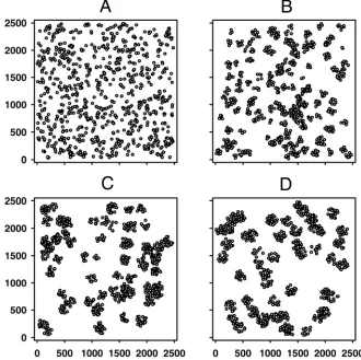
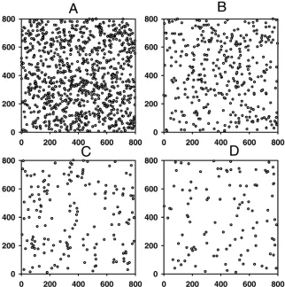
Generation of host landscapes. We generate landscapes of hosts where each host represents a discrete susceptible unit (e.g., a tree, plantation or field). Each landscape consists of 1,000 hosts which are considered to be uniformly susceptible to the disease. To explore the effects of the density and aggregation of the host landscape, we consider 20 landscapes of varying aggregation (Fig. 1) and 18 random host landscapes of varying density (Fig. Corresponding author: S. Parnell; E-mail address: [email protected]
doi:10.1094 / PHYTO-100-7-0638
2). Selections of the landscapes are chosen to be representative of those used during the parameterization of the model (2) (see next section), and variations of these landscapes are also used to dem-onstrate contrasting results. Host landscapes of varying density are generated by altering the dimensions of the square grid in which the set of 1,000 hosts are confined. Within each grid, hosts are randomly allocated an x- and y-coordinate and hence a loca-tion in Cartesian space. The highest density considered is given by a grid area of 0.7 km2 and the lowest by 5.8 km2 with intermediate increments of 0.3 km2 for the 18 density-varying host populations (Fig. 2). Host landscapes of varying aggregation are generated by simulating a clustered spatial point pattern process (3). The same host density, i.e., square grid size, is used for each aggregated host landscape. Centre positions for a number of clusters are randomly determined and hosts are allocated a random location within a predefined radius of a randomly chosen centre position. The level of aggregation is varied by altering the number of centre positions in each host landscape, i.e., the number of clusters, and then adjusting the radius of each cluster (i.e., the radius around the center position) to maintain a constant within-cluster density of hosts across all aggregated host land-scapes. The lowest level of aggregation is given by a landscape with 1,000 cluster center positions (expectation of 1 host per cluster) with a radius of ≈23 m (approximately equivalent to a random distribution) and the highest by 50 center positions (expectation of 20 hosts per cluster) with a cluster radius of ≈103 m (Fig. 1).
The epidemic and eradication model. The epidemic and eradication model and parameter values follow from that of Cook et al. (2) and Parnell et al. (13) where the reader is referred for further information on model derivation and parameterization.
The simulation process is performed independently on each generated host landscape and proceeds as follows: at t = 0 a single host is randomly chosen to be infected. A number of time steps are then performed in which the remaining hosts can stay susceptible, become infected, or be removed by the eradication process. This continues until all infected hosts are removed and there is no infection remaining in the host population. Each iteration, or time step Δt, represents a single day. The probability that a susceptible host, i, becomes infected in a single day is determined by its distance to all currently infected hosts, j, and declines exponentially with rate parameter, α, and Euclidean dis-tance, dij. We also allow for the primary infection rate, ε, which
represents the density- and distance-independent infection pres-sure from the immigration of inoculum external to the host population. The transmission rate of infection is denoted by β. This gives the following expression
probability i infected at Δt = 1 – exp
(
−βΣN∈ −αdij+ε)
jinfectiousexp
Each infected host remains infectious until it is removed by the eradication program. Hosts become symptomatic following a period of 107 days on average. This represents the number of elapsed days following infection when symptoms are known to be best visualized in the field (6). The time to detectable symptom appearance is drawn from a Weibull distribution with mean and variance informed by data (6) and observations from the field (T. R. Gottwald, personal communication). The Weibull distribution has many advantages over the normal, for example it has greater statistical flexibility and also does not generate negative values which are not realistic when describing events occurring in time.
Fig. 1. Simulated distributions of hosts for different levels of clustering, generated by a clustered spatial point-pattern process. Each host distribution contains
Rounds of host removal occur in intervals of 30 days from a randomly chosen starting point (within the first 30 days of the epidemic) and involve the removal of all symptomatic hosts and all other hosts captured within a predetermined control radius. This is based on an actual plant pathogen eradication protocol in the United States (5). This mimics a situation whereby there is regular surveillance for the pathogen before and after its intro-duction. Due to the primary infection parameter, ε, permanent eradication will not occur in the simulation model. Therefore, we define the point of eradication of the epidemic as the first instance when no infectious hosts are in the population.
We perform 1,000 realizations of the simulation process for each host landscape and repeat this for different control radii. Multiple replicates of the simulation are computationally expen-sive and were achieved using parallel computing resources. The computation time is a function of the number of hosts in the landscape and there is therefore a trade-off between the number of hosts required to generate realistic results and the range of param-eter sets that can be analyzed. In the current paper, we choose to focus on the effect of the spatial characteristics of the landscape and choose fixed but informed values for the epidemiological and eradication parameters (2). We also consider variations of the epidemiological parameter values to illustrate the robustness of the main results to them. For each realization, we record the number of hosts removed by the eradication process and also the duration of the epidemic (i.e., the number of elapsed days be-tween the initial infection and the point of eradication).
RESULTS
The results show that a clear optimum control radius can be identified for each host landscape analyzed (Fig. 3A and B). That
is, for each host landscape, very small and very large control radii lead to a high number of host removals during eradication. However, there exists an intermediate length of control radius which minimizes the number of hosts removed. We refer to this length of control radius as the optimum control radius.
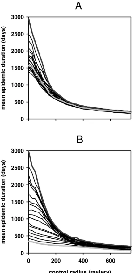
We show that the optimum control radius differs depending on the level of aggregation and density of hosts in the landscape (Fig. 3A and B). In general, the optimum control radius is larger for landscapes characterized by a high level of aggregation than in those with a low level of aggregation (Fig. 3A). We also find that the total number of hosts removed associated with this optimum increases with the level of aggregation of the landscape (Fig. 3A). For example, for the lowest level of aggregation considered, which is close to a random distribution of hosts, we identify an optimum control radius of approximately 175 m (Fig. 3A). This is associated with a total host removal of approximately 400. How-ever, for the highest level of aggregation considered the optimum radius is almost double this at approximately 300 m and is associated with a total host removal of approximately 525, which represents an ≈24% increase (Fig. 3A). Similarly, host landscapes with increased densities also lead to an increase in the length of the optimum control radius and to an increase in the total number of hosts removed associated with this optimum (Fig. 3B). For the lowest density host landscape considered, the optimum control radius was approximately 200 m and was associated with a total host removal of around 450 (Fig. 3B). However, for the highest density considered the optimum radius increased to almost 600 m and was associated with a total host loss of around 875 hosts. The total duration of the epidemic, i.e., the time from initial infection until eradication is achieved, was also recorded at the end of each simulation run (Fig. 4A and B). Although we find that increases in both the aggregation and density of a host population lead to
Fig. 2. Simulated distributions of hosts for different levels of density, generated stochastically. Each host distribution contains 1,000 hosts. The x- and y-axes
increases in the optimum control radius length and the total number of hosts removed, we find that this is associated with a decrease in the time to eradicate the epidemic (i.e., the epidemic duration) (Fig. 4A and B). That is, the results indicate that epidemics in landscapes with higher levels of aggregation and density are eradicated in shorter time frames but are more costly, in terms of the total number of hosts removed, than those in landscapes of lower density and less aggregation (Fig. 4A and B).
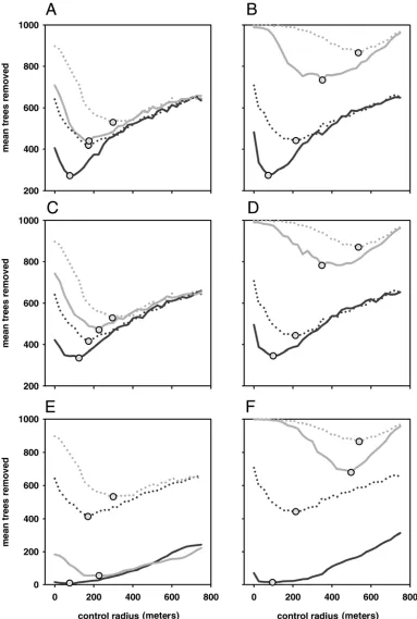
Alternative values of the epidemiological parameters (transmis-sion rate, β; exponent of the dispersal kernel, α; and the rate of primary infection, ε) also led to an increase in the optimum control radius, and the total number of host removals associated with it, with increases in the level of aggregation and density of hosts in the landscape (Fig. 5). For the same host landscapes, the transmission rate, β, exponent of the dispersal kernel, α, and rate
of primary infection, ε, were altered to reduce the rate of increase of the epidemic and consequently each led to a decrease in the optimum control radius and the number of host removals (Fig. 5). However, for high values of control radius the number of host removals was the same for all values of transmission rate, β, and dispersal kernel, α, for the same landscapes (Fig. 5). In contrast, different values of the primary infection rate, ε, led to different numbers of host removals regardless of the control radius (Fig. 5). An exception to this was observed for the landscape of the highest density where very low and very high control radii led to almost all hosts being removed irrespective of the rate of primary infection (Fig. 5). The affects of a number of further epidemio-logical parameter combinations were investigated but were not found to deviate from the qualitative behaviors described above (data not shown).
Fig. 3. The mean number of hosts removed during eradication for different
lengths of control radius. A, The effect of varying the level of clustering of hosts. The light gray line denotes the highest level of clustering and the dark gray line denotes the lowest level of clustering. Black lines are intermediate levels of clustering. B, The effect of varying the density of hosts. The light gray line denotes the highest density analyzed and the dark gray line denotes the lowest density analyzed. Black lines are intermediate densities. Gray dots denote the position of the optimum control radii (unsmoothed curves; shown for highest and lowest density/aggregation landscapes only). Default param-eter values are α = 0.027, β = 0.01, and ε = 4 × 10⁻⁵. Results are averages
from 1,000 realizations of the simulation process.
Fig. 4.The mean duration of the epidemic for different lengths of control
radius. A, The effect of varying the level of clustering of hosts. The light gray line denotes the highest level of clustering and the dark gray line denotes the lowest level of clustering. Black lines are intermediate levels of clustering. B,
The effect of varying the density of hosts. The light gray line denotes the highest density analyzed and the dark gray line denotes the lowest density analyzed. Black lines are intermediate densities. Default parameter values are
α = 0.027, β = 0.01, and ε = 4 × 10⁻⁵. Results are averages from 1,000
DISCUSSION
Recent studies have shown that epidemiological models can be used to identify an optimum control radius for an eradication campaign; that is, an intermediate radius which minimizes the
number of hosts removed (4,13). The central message of this paper is that this depends critically on landscape pattern (i.e., the density and configuration of susceptible hosts within a land-scape). Further, we find that landscape pattern not only has a strong influence on the length of the optimum control radius but
Fig. 5. The mean number of hosts removed during eradication for different lengths of control radius for altered epidemiological parameter values (solid lines
denote altered parameter values and dotted lines denote default parameter values). The left plots are results for landscapes varying in the level of clustering (A, C,
and E) and the right plots are results for landscapes varying in density (B, D, and F). The light gray lines denote the highest level of clustering or the highest
also on the total number of host removals associated with it. Thus, depending on landscape pattern, even the optimal strategy may be deemed an unfeasible and unacceptable option by policy makers. (However, although for epidemics capable of rapid spread the number of hosts removed can be high as a proportion of the hosts in the landscape, we only consider a landscape surrounding a single outbreak. The costs of eradicating this outbreak need to be put in context with the benefit of preventing spread to hosts in other areas.) Specifically, the length of the optimum control radius, and the number of host removals, increases with both aggregation and density (Fig. 3A and B). Studies have shown that host aggregation can lead to decreased epidemic expansion due to the limitation it imposes on local spread (i.e. between-cluster spread) (1,12). Thus, intuition may imply that a shorter control radius be used to eradicate an epidemic in an aggregated landscape, however, we find the contrary to this (Fig. 3A). This can be understood as follows: although the within-cluster rate of epidemic spread is high, it requires a rarer long range dispersal event for an epidemic to jump out of the cluster to the rest of the host population. That is, within-cluster spread occurs much quicker than between-cluster spread. The optimal strategy is therefore to deploy a large control radius to ensure the early re-moval of the cluster of hosts where infection has been found in order to minimize the probability that infection escapes out of the cluster to the rest of the host population. Thus, we find aggregated landscapes are associated with increased lengths of optimum control radii (Fig. 3A) and reduced epidemic durations (Fig. 4A). For landscapes with higher densities of hosts we also find that the length of the optimum control radius and the number of host removals increases. Intuition would suggest that in high density populations it would be optimal to reduce the length of control radius of eradication because so many more hosts would be removed per detected individual than in a lower density popu-lation. However, we show that this not the case. The local spread of an epidemic is facilitated by increased density (due to the decreased distances between neighboring hosts) and therefore a longer control radius is required to contain local spread. This typically controls the epidemic quickly (Fig. 4B) but results in a high number of host removals (Fig. 3B).
Although the parameter choices in the current paper were estimated from data sets of citrus canker disease the key results from the study are robust to different epidemiological parameter values (Fig. 5). That is, the optimum control radius and the total number of host removals associated with it, increase with the level of aggregation and with the density of the hosts in the landscape (Fig. 5). Generally, for the same host landscapes, increases in each of the epidemiological parameters also lead to an increase in the optimum control radius and the number of re-movals associated with it (Fig. 5). For values of the epidemio-logical parameters which lead to a very rapid increase in the epidemic the optimum radius will be less pronounced as all con-trol radii will result in the removal of almost all hosts. Conversely, for epidemiological parameters which lead to a very slow epi-demic increase very few hosts will be removed and the optimum radius will approach zero, i.e., it will only be necessary to remove symptomatic hosts in order to eradicate the epidemic. Neither of these extremes is likely to be exhibited in practice but the results shown here shed light on the spectrum of possible outcomes that are of practical relevance.
The results show that for the same host landscapes, if the control radius is long enough, different transmission rates and dispersal kernels lead to the same number of host removals (Fig. 5). This was not the case for different rates of primary infection however (Fig. 5). The transmission rate and dispersal kernel mainly influence local spread and this is what the control radius acts on. If the control radius oversteps a large cluster of disease it will also overstep a smaller cluster of disease. Thus, for a large enough control radius the same number of hosts are removed
regardless of the extent of local spread. The rate of primary infection influences the number of local clusters of disease, not their size, and thus the same effect does not occur, i.e., for different rates of primary infection there is no control radius that leads to the same number of host removals. For this reason the number of hosts removed is particularly sensitive to the rate of primary infection. This is not surprising because even rare long-distance infection events (i.e., primary infection events) have been shown to be key drivers of epidemic dynamics due to their role in establishing new disease foci in susceptible host areas (9–11). Thus, increases in the rate of primary infection lead to large in-creases in the number of hosts removed during eradication (Fig. 5). In this paper, we have used a simple definition of the optimum control radius, i.e., that which minimizes the mean number of hosts removed during eradication, in order to illustrate the impact of landscape pattern on an optimal eradication strategy. More complicated approaches using multiple criteria will be explored in future work (for example, by incorporating the duration of the epidemic, multiple types of host, sampling costs, and variability in the number of removals) the specific effect of which will depend on the allocation of costs between the various criterion. In the current study we choose to determine density by changing the size of the landscape area and holding the number of hosts con-stant. An alternative approach is to change the number of hosts and hold the size of the landscape area constant. A number of simulations were performed to test this but none were found to qualitatively change the results. Other extensions of the current work include the analysis of the model results for variations in the length of the asymptomatic period, the period between surveys, and the delay between detection and removal. The delay between detection and removal will be of particular importance. For ex-ample, in the recent citrus canker eradication program delays of up to 120 days occurred due to the logistics of moving equipment and survey crews around in addition to legal obstacles in ob-taining permission to enter private properties (5,7). Although out-side the scope of the current study this delay will allow for additional rounds of dispersal and infection to occur and thus increase the optimum control radius and the number of host removals associated with it.
ACKNOWLEDGMENTS
Rothamsted receives support from the Biotechnology and Biological Sciences Research Council (BBSRC). C. A. Gilligan gratefully acknowl-edges a BBSRC professorial fellowship. Part of this work was funded by the U.S. Animal and Plant Health Inspection Service (USDA-APHIS).
LITERATURE CITED
1. Condeso, T. E., and Meentemeyer, R. K. 2007. Effects of landscape heterogeneity on the emerging forest disease sudden oak death. J. Ecol. 95:364-375.
2. Cook, A. R., Gibson, G. J., Gottwald, T. R., and Gilligan, C. A. 2008. Constructing the effect of alternative intervention strategies on historic epidemics. J. Roy. Soc. Interface 5:1203-1213.
3. Diggle, P. J. 2003. Statistical Analysis of Spatial Point Patterns. 2nd ed. Arnold, London.
4. Dybiec, B., Kleczkowski, A., and Gilligan, C. A. 2004. Controlling dis-ease spread on networks with incomplete knowledge. Phys. Rev. E 70:5. 5. Gottwald, T. R., Hughes, G., Graham, J. H., Sun, X., and Riley, T. 2001.
The citrus canker epidemic in Florida: The scientific basis of regulatory eradication policy for an invasive species. Phytopathology 91:30-34. 6. Gottwald, T. R., Sun, X., Riley, T., Graham, J. H., Ferrandino, F., and
Taylor, E. L. 2002. Geo-referenced spatiotemporal analysis of the urban citrus canker epidemic in Florida. Phytopathology 92:361-377.
7. Graham, J. H., Gottwald, T. R., Cubero, J., and Achor, D. S. 2004. Xanthomonas axonopodis pv. citri: Factors affecting successful eradi-cation of citrus canker. Mol. Plant Pathol. 5:1-15.
9. Kot, M., Lewis, M. A., and van den Driessche, P. 1996. Dispersal data and the spread of invading organisms. Ecology 77:2027-2042.
10. Lewis, M. A. 1997. Variability, patchiness, and jump dispersal in the spread of an invading population. Pages 46-69 in: Spatial Ecology: The Role of Space in Population Dynamics and Interspecific Interactions. D. Tilman and P. Kareiva, eds. Princeton University Press, Princeton, NJ. 11. Neubert, M. G., and Caswell, H. 2000. Demography and dispersal:
Calculation and sensitivity analysis of invasion speed for structured populations. Ecology 81:1613-1628.
12. Ostfeld, R. S., Glass, G. E., and Keesing, F. 2005. Spatial epidemiology: An emerging (or re-emerging) discipline. Trends Ecol. Evol. 20:328-336. 13. Parnell, S., Gottwald, T. R., van den Bosch, F., and Gilligan, C. A. 2009.
Optimal strategies for the eradication of Asiatic citrus canker in hetero-geneous host landscapes. Phytopathology 99:1370-1376.
14. Prospero, S., Hansen, E. M., Grunwald, N. J., and Winton, L. M. 2007. Population dynamics of the sudden oak death pathogen Phytophthora ramorum in Oregon from 2001 to 2004. Mol. Ecol. 16:2958-2973. 15. Tildesley, M. J., and Keeling, M. J. 2008. Modelling foot-and-mouth
disease: A comparison between the UK and Denmark. Preventive Vet. Med. 85:107-124.