https://doi.org/10.5194/bg-15-2361-2018 © Author(s) 2018. This work is distributed under the Creative Commons Attribution 4.0 License.
Interannual drivers of the seasonal cycle of CO
2
in the Southern Ocean
Luke Gregor1,2, Schalk Kok3, and Pedro M. S. Monteiro1
1Southern Ocean Carbon-Climate Observatory (SOCCO), CSIR, Cape Town, South Africa 2University of Cape Town, Department of Oceanography, Cape Town, South Africa 3University of Pretoria, Department of Mechanical and Aeronautical Engineering,
Pretoria, South Africa
Correspondence:Luke Gregor (luke.gregor@uct.ac.za)
Received: 25 August 2017 – Discussion started: 20 September 2017
Revised: 9 March 2018 – Accepted: 14 March 2018 – Published: 19 April 2018
Abstract. Resolving and understanding the drivers of vari-ability of CO2in the Southern Ocean and its potential
cli-mate feedback is one of the major scientific challenges of the ocean-climate community. Here we use a regional ap-proach on empirical estimates ofpCO2to understand the role
that seasonal variability has in long-term CO2changes in the
Southern Ocean. Machine learning has become the preferred empirical modelling tool to interpolate time- and location-restricted ship measurements ofpCO2. In this study we use
an ensemble of three machine-learning products: support vector regression (SVR) and random forest regression (RFR) from Gregor et al. (2017), and the self-organising-map feed-forward neural network (SOM-FFN) method from Land-schützer et al. (2016). The interpolated estimates of1pCO2
are separated into nine regions in the Southern Ocean defined by basin (Indian, Pacific, and Atlantic) and biomes (as de-fined by Fay and McKinley, 2014a). The regional approach shows that, while there is good agreement in the overall trend of the products, there are periods and regions where the con-fidence in estimated1pCO2is low due to disagreement
be-tween the products. The regional breakdown of the data high-lighted the seasonal decoupling of the modes for summer and winter interannual variability. Winter interannual vari-ability had a longer mode of varivari-ability compared to sum-mer, which varied on a 4–6-year timescale. We separate the analysis of the1pCO2and its drivers into summer and
win-ter. We find that understanding the variability of1pCO2and
its drivers on shorter timescales is critical to resolving the long-term variability of1pCO2. Results show that1pCO2
is rarely driven by thermodynamics during winter, but rather
by mixing and stratification due to the stronger correlation of 1pCO2variability with mixed layer depth. SummerpCO2
variability is consistent with chlorophyllavariability, where higher concentrations of chlorophyllacorrespond with lower pCO2concentrations. In regions of low chlorophylla
con-centrations, wind stress and sea surface temperature emerged as stronger drivers of1pCO2. In summary we propose that
sub-decadal variability is explained by summer drivers, while winter variability contributes to the long-term changes asso-ciated with the SAM. This approach is a useful framework to assess the drivers of1pCO2but would greatly benefit from
improved estimates of1pCO2and a longer time series.
1 Introduction
The Southern Ocean plays a key role in the uptake of an-thropogenic CO2 (Khatiwala et al., 2013; DeVries et al.,
2017). Moreover, it has been shown that the Southern Ocean is sensitive to anthropogenically influenced climate variabil-ity, such as the intensification of the westerlies (Le Quéré et al., 2007; Lenton et al., 2009; Swart and Fyfe, 2012; DeVries et al., 2017). Until recently, the research community has not been able to quantify the contemporary changes of CO2in
the Southern Ocean accurately due to a paucity of observa-tions, let alone understand the drivers (Bakker et al., 2016). Empirical models provide an interim solution to this chal-lenge until prognostic ocean biogeochemical models are able to represent Southern Ocean CO2fluxes adequately (Lenton
The research community agrees on large changes in CO2
fluxes in the Southern Ocean from a weakening sink in the 1990s to a strengthening sink in the 2000s; however, there is disagreement over the drivers of the changes in CO2uptake
(Lovenduski et al., 2008; Landschützer et al., 2015; DeVries et al., 2017; Ritter et al., 2017). This study aims to under-stand the drivers of the changing CO2sink in the Southern
Ocean, based on an ensemble of empirical estimates using a seasonal analysis framework.
Empirical methods estimate CO2by extrapolating sparse
ship-based CO2 measurements using proxy variables. The
proxies are often observable by satellite but may include climatologies or output from assimilative models. Empirical methods have improved our understanding of CO2trends in
the Southern Ocean by increasing the data coverage. How-ever, there is still disagreement between many of the methods due to the paucity of data and the way in which each method interpolates sparse data (Rödenbeck et al., 2015; Ritter et al., 2017).
In a key study, Landschützer et al. (2015) showed, using an artificial neural network (ANN), that there was signif-icant strengthening of Southern Ocean CO2 uptake during
the period 2002–2010. While previous studies suggested that changes in wind strength have led to changes in meridional overturning and thus CO2uptake (Lenton and Matear, 2007;
Lovenduski et al., 2007; Lenton et al., 2009; DeVries et al., 2017), Landschützer et al. (2015) suggested that atmospheric circulation has become more zonally asymmetric since the mid-2000s, which has led to an oceanic dipole of cooling and warming. The net impact of cooling and warming, together with changes in the DIC and TA (dissolved inorganic carbon and total alkalinity), led to an increase in the uptake of CO2
(Landschützer et al., 2015). During this period, southward advection in the Atlantic basin reduced upwelled DIC in sur-face waters, overcoming the effect of the concomitant warm-ing in the region. Conversely, in the eastern Pacific sector of the Southern Ocean, strong cooling overwhelmed increased upwelling (Landschützer et al., 2015). This is supported by observations from the Drake Passage and south of Australia showing that variability of upwelling has affected 1pCO2
(Munro et al., 2015; Xue et al., 2015).
In a subsequent study, Landschützer et al. (2016) proposed that interannual variability of CO2 in the Southern Ocean
is tied to the decadal variability of the Southern Annular Mode (SAM) – the dominant mode of atmospheric variabil-ity in the Southern Hemisphere (Marshall, 2003). This con-curs with previous studies, which suggested that the increase in the SAM during the 1990s resulted in the weakening of the Southern Ocean sink (Le Quéré et al., 2007; Lenton and Matear, 2007; Lovenduski et al., 2007; Lenton et al., 2009; Xue et al., 2015). The work by Fogt et al. (2012) bridges the gap between the proposed asymmetric atmospheric cir-culation of Landschützer et al. (2015) and the observed cor-relation with the SAM of Landschützer et al. (2016). Fogt et al. (2012) show that changes in the SAM have been
zon-ally asymmetric and that this variability is highly seasonal, thus amplifying or suppressing the amplitude of the seasonal mode.
Assessing the changes through a seasonal framework may thus help shed light on the drivers of CO2 in the
South-ern Ocean. SouthSouth-ern Ocean seasonal dynamics suggest that the processes drivingpCO2are complex, but with two clear
contrasting extremes. In winter, the dominant deep mixing and entrainment processes are zonally uniform, driving an increase inpCO2, with the region south of the Polar Front
(PF) becoming a net source and weakening the net sink north of the PF (Lenton et al., 2013). In summer, the picture is more spatially heterogeneous, with net primary production being the primary driver of variability (Mahadevan et al., 2011; Thomalla et al., 2011; Lenton et al., 2013). The com-peting influence between light and iron limitation results in heterogeneous distribution of chlorophylla (Chla) in both space and time, with similar implications forpCO2
(Thoma-lla et al., 2011; Carranza and Gille, 2015). The interaction between the large-scale drivers, such as wind stress, sur-face heating, and mesoscale ocean dynamics, are the primary cause of this complex picture (McGillicuddy, 2016; Mahade-van et al., 2012). Some regions of elevated mesoscale and sub-mesoscale dynamics, mainly in the Sub-Antarctic Zone (SAZ), are also characterized by strong intra-seasonal modes in summer primary production andpCO2 (Thomalla et al.,
2011; Monteiro et al., 2015). In general, the opposing effects of mixing and primary production result in the seasonal cy-cle being the dominant mode of variability in the Southern Ocean (Lenton et al., 2013).
In this study we examine winter and summer interannual variability of1pCO2in the Southern Ocean between 1998
and 2014 to understand the drivers of long-term changes in CO2uptake.
2 Methodology
2.1 Empirical methods and data
The SVR and RFR implementations used in this study are trained with the monthly 1 by 1◦gridded SOCAT
(Sur-face Ocean CO2Atlas) v3 dataset (Bakker et al., 2016). The
SOM-FFN (run ID:netGO5) used in this study was trained with SOCAT v4 (Landschützer et al., 2017).
Table 1 shows the proxy variables used for each of the methods. Sea surface salinity (SSS) and mixed layer depth (MLD) for SVR and RFR are from Estimating the Circula-tion and Climate of the Ocean, Phase II (ECCO2)
(Mene-menlis et al., 2008). The use of these assimilative modelled products may in some cases produce results that are unre-alistic. This may have influenced the use of the de Boyer Montégut et al. (2004) MLD climatology in the SOM-FFN, where ECCO2 was used in previous iterations of the
prod-uct. The trade-off of using the climatology is that no in-terannual changes in MLD are taken into account. We ac-knowledge that using different proxy variables could re-sult in different 1pCO2 estimates, but comparing the
dif-ferent proxies used in each of the CO2 products is beyond
the scope of this study. Other data sources that are con-sistent between methods are sea surface temperature (SST) and sea-ice fraction by Reynolds et al. (2007), Chl a by Maritorena and Siegel (2005), absolute dynamic topogra-phy (ADT) generated by DUACS and distributed by AVISO (ftp://ftp.aviso.oceanobs.com, last access: 12 July 2012), and xCO2(CDIAC, 2016) withpCO2(atm)calculated from inter-polated xCO2 using NCEP2 sea level pressure (Kanamitsu
et al., 2002). In the case of Chlafor SVR and RFR, Gregor et al. (2017) filled the cloud gaps with climatological Chla. Note that ADT coverage is limited to regions of no to very low concentrations of sea-ice cover, so estimates for SVR and RFR do not extend into the ice-covered regions during winter. Our analyses are thus limited to the region north of the maximum sea-ice extent.
Seasonality of the data is preserved by transforming the day of the year (j) and is included in both SVR and RFR analyses: t= cos
j· 2π 365
sin
j· 2π 365 . (1)
Transformed coordinate vectors are passed to SVR only usingn-vector transformations of latitude (λ) and longitude (µ) (Gade, 2010; Sasse et al., 2013), withN containing the following:
N =8
sin(λ)
sin(µ)·cos(λ) −cos(µ)·sin(λ)
(2)
Wind speed, while not used in the empirical methods, is used in the assessment of the drivers of CO2. We use CCMP
v2, which is an observation-based product that combines re-mote sensing, ship, and weather buoy data (originally pub-lished by Atlas et al., 2011 and updated by Wentz et al.,
2015). Swart et al. (2015a) compared a number of wind re-analysis products with CCMP v1 (where CCMP was the benchmark). The authors found that many of the reanaly-sis products had spurious trends, particularly in the South-ern Hemisphere where data are sparse. Our choice of CCMP, which is based on observations, aims to minimise the as-sumptions that are otherwise made by reanalysis products. 2.2 Uncertainties
The machine-learning approaches used in this study are by no means able to estimate1pCO2 with absolute certainty.
To account for the uncertainty, we use the same approach as Landschützer et al. (2014) to calculate total errors for each of the methods:
e(t )= q
e2
meas+egrid2 +e2map, (3)
whereem(t )is the total error associated with a method (m); emeas is the error associated with SOCAT measurements,
which is fixed at 5 µatm (Pfeil et al., 2013), where 1 µatm is 101 325 Pa;egrid is the 5 µatm error associated with
grid-ding the data into monthly by 1◦bins (Sabine et al., 2013).
Lastlyemapis the root mean squared error (RMSE) calculated
for each method, as shown in Table 1 taken from Gregor et al. (2017).
These errors are used to calculate the average “within-method” error as defined by Gurney et al. (2004):
Ew=
r 1 M·
XM m=1 em(t )
2
, (4)
whereem(t )is the method-specific error as defined in Eq. (3) andM is the number of methods (three in this case). For a measure of the difference between methods we use the “between-method” approach used in Gurney et al. (2004):
Eb=
r 1 M·
XM
m=1 Sm−S
2
, (5)
whereSm is the method estimate of 1pCO2 and S is the
mean of the methods. This is analogous to the standard devi-ation (for a known populdevi-ation size). We later use an adapta-tion of this metric as a threshold to determine the confidence around anomalies.
2.3 Regional coherence framework
Southern Ocean CO2is spatially heterogeneous, both zonally
Table 1. Three empirical methods used in the ensemble. RFR and SVR are described in Gregor et al. (2017). SOM-FFN is from Land-schützer et al. (2016). SST=sea surface temperature, MLD=mixed layer depth, SSS=sea surface salinity, ADT=absolute dynamic topography, Chla=chlorophylla,pCO2(atm)=fugacity of atmospheric CO2,xCO2(atm)=mole fraction of atmospheric CO2,8(lat.,
long.)=N−vector transformations of latitude and longitude,t(day of year)=trigonometric transformation of the day of the year. Note that SOM-FFN uses the de Boyer Montégut et al. (2004) climatology for MLD (dBM2004). The root mean squared errors (RMSEs) listed in the last column are for the Southern Ocean from Gregor et al. (2017).
Method Input variables RMSE (µatm) RFR SST, MLD, SSS, ADT, Chl-a(clim),pCO2(atm),8(lat., long.),t(day of year) 16.45 SVR SST, MLD, SSS, ADT, Chl-a(clim),pCO2(atm),8(lat., long.),t(day of year) 24.04 SOM-FFN SST, MLDdBM2004, SSS, Chla,xCO2(atm) 14.84
used throughout the rest of the study. The Southern Ocean is further split into basins where the boundaries are defined by lines of longitude (70◦W – Atlantic – 20◦E – Indian – 145◦E – Pacific – 70◦W).
3 Results and discussion
The first section of the results examines the uncertainties of the ensemble and its members. We then look at the seasonal cycle of the ensemble mean in time and space. This is done to lay the foundation for the interpretation of the results when assessed with the regional framework. In the regional inter-pretation the estimates are decomposed into nine regions, as shown in Fig. 1. Lastly, we implement a seasonal decompo-sition of the estimates to interpret the drivers of the changes observed in1pCO2.
3.1 Ensemble member performance and variability
We use the RMSE scores as presented in Gregor et al. (2017) with abbreviated results shown in Table 1. The SOM-FFN method has the best score (14.84 µatm). SVR scores the low-est (24.04 µatm), but is still included due to the method’s sensitivity to sparse data, which is favourable to the poorly sampled winter period (Gregor et al., 2017). This compli-ments the RFR method, which scores well (16.45 µatm) but is prone to being insensitive to sparse data (Gregor et al., 2017). These RMSE scores are used to calculate the total errors for each method and region using Eq. (3), where the measurement and mapping errors are both 5 µatm each (Pfeil et al., 2013; Sabine et al., 2013). These results are shown in Table 2.
[image:4.612.320.533.219.452.2]Total errors are used to calculate the within-method error, which is an estimate of the combined total error of the three machine-learning methods (Eq. 4). The between-method er-rors are the mean of the standard deviation between the meth-ods (Eq. 5). The within-method errors are much larger than the between-method errors (Table 2). However, the within-method errors are normally distributed and are mechanisti-cally consistent (Gregor et al., 2017). The between-method
Figure 1.A map showing the regions used throughout this study. The three biomes used in this study, SAZ, PFZ, and MIZ, are de-fined by Fay and McKinley (2014a). The regions are also split by basin.
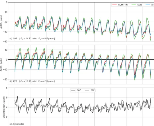
error (shown in Fig. 2c) is thus used to determine whether observed variability is consistent between the three methods. Figure 2 shows the1pCO2time series for the SAZ and
PFZ. Note that we exclude the MIZ from the remaining analyses due to large Eb and Ew (Table 2) and inconsis-tent coverage between products due to sea-ice cover (MIZ data are shown in the Supplement S2, S4). In general, there is good agreement amongst the methods and the magnitude of these differences is within the average within-method er-ror (Ew), but the differences are important to highlight as they contribute to the between-method error (Eb). In the SAZ (Fig. 2a), the SOM-FFN differs from the other meth-ods for summer and autumn from 1998 to 2008. The SVR method overestimates the seasonal amplitude1pCO2(where
Table 2.A regional summary of the errors for the different methods. Note that the propagated errors are calculated as shown in Eq. (3) where the measurement and gridding errors are assumed to be constant at 5 µatm each (Pfeil et al., 2013; Sabine et al., 2013). The within-method and between-method errors are calculated using Eqs. (4) and (5) respectively.
Propagated errors (µatm)
Biome SVR RFR SOM- Within- Between-FFN method error method error (µatm) (µatm) SAZ 17.48 14.50 12.30 14.91 4.88 PFZ 15.94 12.71 13.09 13.99 4.78 MIZ 36.38 24.53 22.46 28.46 10.81 Southern Ocean 25.06 17.91 16.44 20.16 6.79
methods for 2012 to 2014. In the PFZ (Fig. 2b), the SVR overestimates 1pCO2relative to the other methods during
winter from 1998 to 2004, likely due to the method’s sensi-tivity to sparse winter data (Gregor et al., 2017).
Figure 2c shows the time evolution of between-method er-rors for each biome. This panel highlights the seasonality of the estimates, specifically the increased heterogeneity of 1pCO2in summer and the impact this has on1pCO2
esti-mates. This is due to the more complex competing processes affectingpCO2during summer. To gain a better
understand-ing of the seasonal processes, we consider the mean state of each season to characterise the drivers of opposing fluxes.
3.2 Ensemble seasonal cycle
The seasonal cycle of the1pCO2for each biome (Figs. 2a–b
and 3a–d) is coherent with seasonal processes reported in the literature (Metzl et al., 2006; Thomalla et al., 2011; Lenton et al., 2012, 2013). In all biomes, uptake of CO2is stronger
dur-ing summer than in winter, givdur-ing rise to the strong seasonal cycle. This is due to the opposing influences of the domi-nant winter and summer drivers, partially damped by the sea-sonal cycle of temperature (Takahashi et al., 2002; Thoma-lla et al., 2011; Lenton et al., 2013). In winter, the domi-nant processes of mixing and entrainment results in increased surface pCO2 and thus outgassing (Takahashi et al., 2009;
Lenton et al., 2013; Rodgers et al., 2014). In summer, strat-ification allows for increased biological production and the consequent uptake of CO2, thus reducing the entrained
win-ter DIC and associatedpCO2(Bakker et al., 2008; Thomalla
et al., 2011). However, stratification typically limits entrain-ment other than during periods of intense mixing driven by storms. This has an impact on primary productivity, DIC and pCO2(Lévy et al., 2012; Monteiro et al., 2015; Nicholson et
al., 2016; Whitt et al., 2017).
The SAZ (Fig. 2a) is a continuous sink, where summer uptake (Fig. 3a) is enhanced by biological production and winter (Fig. 3c) mixing results in a weaker sink (Metzl et al., 2006; Lenton et al., 2012, 2013). The same processes pro-duce a similar seasonal amplitude in the PFZ (Fig. 2b), but
stronger upwelling and weaker biological uptake result in a positive shift of the mean. This results in an opposing net summer sink and winter source. However, this is according to the mean state in the PFZ, and winter estimates of1pCO2
do in fact approach 0 µatm toward the end of the time series (Fig. 2b).
Also apparent from Fig. 3 is that, over and above the latitudinal gradient, 1pCO2 is zonally asymmetric within
each biome during summer (Fig. 3a), when biological up-take of CO2 increases. Zonal integration of 1pCO2 could
thus dampen magnitudes of regional1pCO2. A regional
ap-proach is therefore needed to examine the regional character-istics of seasonal and interannual variability of1pCO2and
to understand its drivers.
3.3 Regional1pCO2variability: zonal and basin contrasts
In Fig. 4,1pCO2is decomposed into nine domains by biome
and basin, with the boundaries defined in Fig. 1 (showing the SAZ and PFZ; air–sea CO2fluxes displayed in Fig. S4 in the
Supplement). The regional estimates are plotted as time se-ries for1pCO2(black lines). The blue and orange lines show
the respective annual maxima (typically winter) and minima (typically summer). The projected summer minima (dashed blue lines) are calculated by subtracting the mean seasonal amplitude from the winter maxima (Fig. 4). The projected summer minima are the expected summer1pCO2under the
assumption that summer1pCO2is dependent on, but not
re-stricted to, the baseline set by winter.
As found by Landschützer et al. (2015), the estimates of 1pCO2(Fig. 4) show that the Southern Ocean sink
strength-ens from 2002 to 2011 in all domains, referred to as the rein-vigoration. This is preceded by a period of a net weakening sink (Fig. 4b, d, e) in the 1990s, referred to as thesaturation
between-Figure 2.Time series of the three ensemble methods for each biome, as defined by Fay and McKinley (2014a):(a)SAZ,(b) PFZ and (c)the standard deviation between ensemble members for the three biomes, which is analogous to the between-method error (Eq. 5). The within-method (Ew)and between-method (Eb)errors are shown for each biome. For a more detailed breakdown of the errors see Table 2.
method error in Fig. 4 (see Fig. S4 for the spread of the prod-uct estimates, including the Jena mixed layer scheme by Rö-denbeck et al., 2014). This disagreement between methods is likely driven by the sparse coverage ofpCO2measurements
in the Southern Ocean, with empirical methods interpolat-ing the sparse data differently (Rödenbeck et al., 2015; Ritter et al., 2017). We thus present our methods and results as a framework to assess the drivers of interannual variability of 1pCO2.
Key to understanding the mean interannual variability is that it is the net effect of the decoupled seasonal modes of variability for summer and winter. This is particularly evident in the PFZ (Fig. 4d–f). Here, and in the other biomes, the net strengthening of the CO2sink is mainly linked to a reduction
of1pCO2in winter for the majority of the time series. This
corresponds with the findings of Landschützer et al. (2016), who linked the reinvigoration to the decadal variability of the SAM – the dominant mode of atmospheric variability in the Southern Hemisphere (Marshall, 2003). In contrast, sum-mer1pCO2variability is shorter (roughly 4–6 years), thus
providing interannual modulation of longer-timescale winter variability. This is demonstrated well in the Indian sector of the PFZ, where a decrease in winter1pCO2from 2002 to
2011 is offset by weakening of the summer sink from 2006 to 2010 (Fig. 4d). Similarly, in the Atlantic and Pacific sec-tors of the PFZ, decoupling occurs from∼2011 to the end of 2014, with a rapid increase in the strength of the summer sink.
The mean amplitude of the seasonal cycle of1pCO2– the
[image:6.612.52.548.66.472.2]win-Figure 3.The mean seasonal states of1pCO2of the empirical ensemble mean. These are shown for(a)summer,(b)autumn,(c)winter, and
[image:7.612.128.469.71.356.2](d)spring. The black contour lines show the SAZ, PFZ, and MIZ (masked) from north to south, as defined by Fay and McKinley (2014a).
Figure 4.Panels(a–f)show the ensemble mean of1pCO2(black) plotted by biome (rows) and basin (columns). Biomes are defined by Fay
and McKinley (2014a). The blue line shows the maximum for each year (winter outgassing) and the dashed blue line shows the same line less the average seasonal amplitude (diff)– this is the expected amplitude. The orange line shows the minimum1pCO2for each summer
season. The shaded regions around the seasonal maxima and minima show the standard deviation of the three products.Ebis the average between-method error and1pCO2is the average for the entire time series. Light grey shading in(a–f)shows the periods used in Figs. 5 and
[image:7.612.71.522.411.637.2]ter maxima – is perhaps a better way of understanding the strength of the seasonal drivers than the mean1pCO2. For
example, the Atlantic sectors of the SAZ and PFZ (Fig. 4c, f) have the strongest seasonal variability (14.11 and 25.83 µatm respectively). This contrasts with the relatively weak sea-sonal amplitude in the Indian sector of the Southern Ocean, which has mean amplitudes of 7.06 and 13.64 µatm for the SAZ and PFZ respectively (Fig. 4b, e). This contrast can also be seen by comparing the mean seasonal maps of1pCO2in
Fig. 3a and c. In summer, strong uptake in the eastern At-lantic sector of the Southern Ocean is indicative of large bio-logical drawdown of CO2by phytoplankton (Thomalla et al.,
2011). Conversely, relatively low primary production in the Indian sectors of the SAZ and PFZ result in a small seasonal amplitude (Thomalla et al., 2011). This large discrepancy in biological primary production is related to the availability of iron, a micronutrient required for photosynthesis. The lack of large land masses, which are a source of iron, in the Indian sector of the Southern Ocean could be a contributing factor to the lack of biomass (Boyd and Ellwood, 2010; Thomalla et al., 2011).
3.4 Framework: seasonal deconstruction of interannual variability
Figure 4 gives us insight into the magnitude of interannual 1pCO2variability as well as the character of these changes,
i.e. decoupling of interannual winter and summer modes of variability. This alludes to the point that1pCO2is
respond-ing to different adjustments of seasonal large-scale atmo-spheric forcing and/or responses of internal ocean dynamics in the Southern Ocean (Landschützer et al., 2015, 2016; De-Vries et al., 2017).
In order to capture the decoupled 4–6-year short-term vari-ability observed in summer, the estimates are divided into four objectively selected periods (P1 to P4). The periods are each 4 years long with the exception of P1, which is 5 years long due to the fact that the duration of the time series is not divisible by 4 (with a total duration of 17 years). Given a longer time series, this analysis would benefit from test-ing different durations for each period, as well as varytest-ing the starting and end years.
These four periods are too short for trend analyses (Fay et al., 2014), but the intention here is to identify periods that are short enough to resolve interannual changes of large-scale drivers of the winter and summer pCO2 that would
other-wise be averaged out over longer periods. We then calculate the relative anomaly between each successive period rather than an anomaly of the mean state (e.g. P2–P1). As a result, four periods give rise to three sub-decadal-scale transition anomalies for summer and winter: A(P2–P1), B (P3–P2), andC(P4–P3). We do this separately for each method rather than using the ensemble mean (see Sect. 3.1.4 for calcula-tions). The mean of the method anomalies for each transition is then taken. These anomalies are considered significant if
the absolute estimate of the anomaly is larger than the stan-dard deviation between the methods for each period.
Note that although only summer and winter anomalies are discussed, it is recognised that autumn and spring could be equally mechanistically important. Winter anomalies of 1pCO2, wind stress, SST, and MLD are shown in Fig. 6,
while summer anomalies of1pCO2, wind stress, SST, and
Chla are shown in Fig. 7. Chla is potentially a more im-portant driver in summer than the generally shallow summer MLD (the omitted plots are shown in Figs. S5 and S6). 3.4.1 Uncertainty of transition anomalies
The transition anomalies are not calculated from the mean of the three products. Rather, we calculate the anomalies for each individual product with
an(p0)=Sn(p)−Sn(p−1), (6)
wheres are the estimates for a particular product,n repre-sents an individual product andp represents P1 to P4. The result,an(p0)thus represents the anomaly for two periods for
a particular product. We then calculate the average of the anomalies with
ap0 =
1 N ·
XN
n=1an(p0), (7)
whereN is 3, the number of products. We then calculate the standard deviation of the three anomalies (ep0), which is
anal-ogous to the between-method error, with ep0=
r 1 N ·
XN
n=1 an(p0)−an(p0)
2
, (8)
where the terms are consistent with those above. We useep0
as an uncertainty threshold where anomalies are only con-sidered significant if|ap0|> ep0. These regions are masked
in Figs. 6a–c and 7a–c. Figure 5 shows the winter (a–c) and summer (d–f)ep0 for each transition anomaly.
3.5 Drivers of winter1pCO2variability
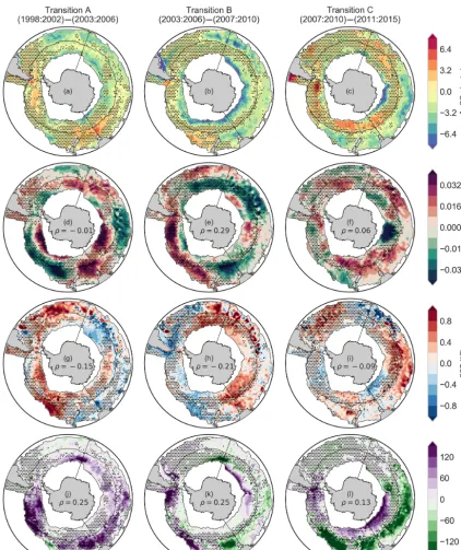
Figure 6 shows the three transition anomalies for the four periods shown in Fig. 4. It is clear that there is large uncer-tainty around the1pCO2anomalies in the Southern Ocean
owing to the differences between the three empirical meth-ods, caused by a paucity of in situ measurements of1pCO2.
However, there are still small regions that show anomalies with confidence. Figure 6d–l also show the Pearson’s correla-tion coefficients for each of the driver variables with1pCO2
for the regions that are above the uncertainty threshold. The correlations in Fig. 6 show that MLD is a dominant predictor ofpCO2in winter (Fig. 6j–l), with wind stress
be-ing a stronger predictor only in Transition B (6e). However, these correlations are all less than|0.3|, indicating that the relationship between1pCO2and MLD is complex and
Figure 5.Maps of the standard deviation between empirical methods for the anomalies. These are used as thresholds for1pCO2in Figs. 6a–c
and 7a–c for winter and summer respectively. When the standard deviation exceeds the absolute value average anomaly, the values are masked, as shown in Figs. 6 and 7.
are applied for the entire domain (above the threshold). This is likely due to MLD being a metric that measures the com-plex interaction of heat, stratification, and mixing processes (Abernathy et al., 2011) – mechanisms relating to SST and wind stress. We now discuss the results by transition.
In Transition A (first column of Fig. 6), MLD is the strongest driver. Deeper mixed layers in the Pacific and east-ern Indian sectors of the Southeast-ern Ocean correspond with in-creased deepening, correlating with inin-creased 1pCO2. The
reduction of1pCO2along the boundary of the Atlantic and
Indian sectors of the SAZ corresponds with increased SST. This agrees with the hypothesis put forward by Landschützer et al. (2015) that warmer SSTs in the Atlantic led to increased uptake of CO2. However, the same is not true for the western
Indian sector of the PFZ, where cooling and deepening MLD results in a reduction of1pCO2.
Increased uptake of 1pCO2 across the boundary of the
Atlantic and Indian sectors of the SAZ continues into Transi-tion B (second column of Fig. 6). This is again accompanied by an increase in SST (Fig. 6h). The reduction of1pCO2
extends to the eastern Indian sector of the SAZ and Tasman Sea. This corresponds with weak shoaling of the MLD, weak warming and a reduction of wind stress (Fig. 6e, h, k). Con-versely, in the eastern Pacific, cooling surface temperatures, weaker winds, and shallower MLDs correspond with a re-duction of1pCO2, again in agreement with Landschützer et
al. (2015). The large reduction of1pCO2in the Indian
sec-tor of the PFZ corresponds with an increase in temperature; however, there is also an increase in the depth of the MLD
– this interaction is mechanistically unlikely and may be an artefact of the sparse data in this region.
In Transition C, the reduction of1pCO2in the Indian and
western Pacific sector of the SAZ corresponds with warmer SST and shallower MLDs. Once again there is a region in the Indian sector of the PFZ that experiences a potentially spuri-ous reduction of1pCO2corresponding with deeper MLDs.
The anomalies in the rest of the domain are not significant.
3.5.1 MLD-driven interannual variability ofpCO2in winter
Our results indicate that there is not one dominant driver of1pCO2interannual transition anomalies in winter. While
MLD is on average the stronger driver, its dominance of 1pCO2is only marginal over SST and wind stress (Fig. 6).
This marginal dominance over the two other drivers is likely due to MLD being a metric that integrates the complex inter-action between wind-driven mixing and winter heat loss to the atmosphere, of which SST is a response (De Boyer Mon-tégut et al., 2004; Sallée et al., 2010). Mechanistically, deeper MLDs would result in greater entrainment of DIC-rich deep waters, while shallower MLDs entrain less DIC-rich waters, thus reducing the DIC pool in winter resulting in potentially stronger1pCO2uptake in the surface ocean (Lenton et al.,
2013).
An important point to note is that SST is negatively corre-lated with1pCO2in Fig. 6g–i. This is contrary to what is
Figure 6.Transitions (relative anomalies) of winter1pCO2(a–c), wind stress(d–f), sea surface temperature(g–i), and mixed layer depth
(j–l)for four periods. The thin black lines show the boundaries for each of the nine regions described by the biomes (Fay and McKinley, 2014a) and basin boundaries. Regions with dots are where1pCO2anomalies are not significant; i.e. standard deviation of the anomalies
between methods are greater than the absolute mean of method anomalies, as described in Eqs. (6)–(8).
al., 1993). This indicates that SST – a response to underlying variability and trends in winter buoyancy and mixing – is not a driver of1pCO2changes in most regions of the Southern
Ocean. There are some small sub-regions, where SST could drive the 1pCO2 trend, such as in the eastern Pacific
sec-tor of the PFZ during Transition B (Fig. 6b, h) but they are
Wind-stress anomalies (Fig. 6d–f) do not correlate strongly withpCO2anomalies, with the exception of
Tran-sition B, when it has the strongest correlation. We propose that this lack of coherence between the two variables may be a result of two compounding points. Firstly, wind stress is the only truly independent driver in the analysis, with SST and MLD both being used as proxies for 1pCO2 in
each of the products. Secondly, the wind stress shown in Fig. 6d–f considers only wind strength, so it does not take into account potential meridional changes in atmospheric cir-culation. This is the primary hypothesis presented in Land-schützer et al. (2015), suggesting that atmospheric circula-tion became more zonally asymmetric. This induced a south-ward shift of warmer waters over the Atlantic and Indian sectors, reducing the depth of the MLD. Conversely, in the eastern Pacific cold winds induced colder SST and thus an increase in solubility.
Past studies have related the variability of Southern Ocean wind stress to the SAM, where the multi-decadal increas-ing trend has been cited as a reason for the saturation in the 1990s (Marshall, 2003; Le Quéré et al., 2007; Lenton and Matear, 2007; Lovenduski et al., 2008). The SAM is often represented as a zonally integrating index (Marshall, 2003), but more recent studies have shown that the SAM, as the first empirical mode of atmospheric variability, is zonally asym-metric (Fogt et al., 2012). The zonal asymmetry of the SAM is thought to be linked with the El Niño–Southern Oscillation and is strongest in winter, particularly over the Pacific sec-tor of the Southern Ocean during a positive phase, in accord with the dipole nature of the Pacific–Indian winter wind-stress transition observed in Fig. 6d, e (Barnes and Hartmann, 2010; Fogt et al., 2012). Fogt et al. (2012) noted that the SAM has become more zonally symmetric in summer since the 1980s, matching the characteristics of the anomalies of wind-stress transitions seen in Fig. 6d–f and the hypothesis of Landschützer et al. (2015).
In summary, our analysis of the drivers of1pCO2is
con-sistent with the atmospheric asymmetry (dipole) conceptual model associated with the SAM proposed by Landschützer et al. (2015). However, our results suggest that interannual 1pCO2trends are explained by DIC dynamics rather than
by the thermodynamic response ofpCO2. A key part of this
emphasis on DIC is that our results indicate that1pCO2and
SST are not correlated in a way that supports a thermody-namic control of1pCO2.The reasons for these differences are not clear at this stage, but they could include differences in the temporal resolution of the two studies: the resolution of the seasonal extremes in this study (seasonal modes) vs. annual mean in Landschützer et al. (2015).
3.6 Anomalies of1pCO2and its summer drivers
Compared to the winter transitions, summer transitions (Fig. 7) have larger areas where the anomalies between prod-ucts are within the bounds of the uncertainty. This may be
due to the larger magnitude of the anomalies in summer com-pared to winter (Fig. 6). In summer we also see that Chla (Fig. 7j–l) is likely the first-order driver with the highest cor-relation scores for transitions A and B.
Transition A (P2–P1 in Fig. 7a) is marked by a decrease of CO2in the SAZ (Tasman shelf region), coinciding with an
increase in Chla. The Drake Passage region experiences a strong reduction of1pCO2in the PFZ, as found by Munro
et al. (2015) and Landschützer et al. (2015). Unlike in the Tasman basin, this reduction of1pCO2is not accompanied
by a strong increase in Chla, but rather a reduction of wind stress and an increase in SST. This is contrary to the annu-ally integrated analysis of Landschützer et al. (2015), who found that cooling drove a reduction ofpCO2in the eastern
Pacific sector of the PFZ. This difference likely arises from the integration of seasons and a longer period (2002–2011) compared to the framework used in this study. In the Indian sector of the PFZ the products agree on a weak increase in 1pCO2corresponding with a weak reduction of Chla.
Transition B (P3–P2 in Fig. 7b) shows a large reduction of 1pCO2 in the Atlantic sector of the PFZ and southern
SAZ. The reduction coincides with an increase in Chla and SST in the same region, in agreement with Landschützer et al. (2015).
In Transition C (P4–P3 in Fig. 7c) the reduction of the 1pCO2 is widespread in the Indian and Pacific oceans in
both biomes, as the increase in Chlais similarly widespread; however, the increase in Chlain the Indian sector of the SAZ is not strong compared to other regions where1pCO2 and
Chlavariability correspond. Conversely, there is a reduction in Chlaand concomitant increase in1pCO2along the Polar
Front in the Atlantic sector, coinciding with the position of the Antarctic Circumpolar Current (ACC) – a region with high eddy kinetic energy (EKE) (Meredith, 2016).
Based on these cases we suggest that1pCO2is driven
pri-marily by Chla in regions with high-Chla concentrations. Note that we will not try to explain Chlavariability, which is complex due to the multitude of factors influencing phyto-plankton growth (Thomalla et al., 2011). We further suggest that in regions of low Chla, buoyancy forcing and mixing are higher-order drivers. As suggested for winter variability, these two mechanisms are a complex interaction of variables of which SST and wind stress are a part (Abernathy et al., 2011).
This then raises the importance of the magnitudes of the interannual variability of1pCO2and its drivers. For
exam-ple, the anomalies of 1pCO2 and SST are larger in
sum-mer than in winter. Conversely, the wind-stress anomalies are larger for winter than in summer. This is an important consideration for analyses that aim to understand the driv-ing mechanisms, where annual averagdriv-ing would weight sea-sonally asymmetric responses of1pCO2and its drivers
Figure 7.Relative anomalies of summer1pCO2(a–c), wind stress(d–f), sea surface temperature(g–i), and mixed-layer depth(j–l)for four
periods (as shown above each column). The thin black lines show the boundaries for each of the nine regions described by the biomes (Fay and McKinley, 2014a) and basin boundaries. Regions with dots are where1pCO2anomalies are not significant; i.e. standard deviation of
the anomalies between methods are greater than the absolute mean of method anomalies, as described in Eqs. (6)–(7).
3.6.1 Chlorophyll-dominated interannual anomalies of pCO2in summer
Our finding that Chlais the dominant driver of interannual 1pCO2variability should not be surprising given that
mod-els and observations support this notion (Hoppema et al.,
1999; Bakker et al., 2008; Mahadevan et al., 2011; Wang et al., 2012; Hauck et al., 2013, 2015; Shetye et al., 2015). How-ever, our data show that the dominance of interannual Chla variability over1pCO2 is largely limited to regions where
Figure 8. Chl a seasonal cycle reproducibility and iron-supply mechanisms in the Southern Ocean. Regions of chlorophyll biomass and seasonal cycle reproducibility from Thomalla et al. (2011) (us-ing SeaWIFS data). Seasonality is calculated as the correlation be-tween the mean annual seasonal cycle compared to the observed chlorophyll time series. A correlation threshold of 0.4 is applied to each time series to distinguish between regions of high and low seasonality; similarly, a threshold of 0.25 mg m−3is used to distin-guish between low or high chlorophyll waters. Black lines showing the fronts are calculated using altimetry thresholds from Swart et al. (2010).
The spatial variability of high Chlaregions in the South-ern Ocean is complex due to the dynamics of light and iron limitation (Arrigo et al., 2008; Boyd and Ellwood, 2010; Thomalla et al., 2011; Tagliabue et al., 2014, 2017). This complexity is highlighted in Thomalla et al. (2011), where the Chl ais characterized into regions of concentration and seasonal cycle reproducibility (SCR; Fig. 8). The SCR is cal-culated as the correlation between the mean annual seasonal cycle and the observed chlorophyll time series. Here we use the approach of Thomalla et al. (2011), in Fig. 8, as a con-ceptual framework to understand the interannual variability of1pCO2.
3.6.2 High-chlorophyll regions
While regions of high SCR (dark green in Fig. 8) do not cor-respond with the interannual variability of Chla(Fig. 7j–l), the framework by Thomalla et al. (2011) does present a hy-pothesis by which the variability of Chlaand its drivers can
be interpreted, i.e. that the variability of Chla in a region is a complex interaction of the response of the underlying physics (mixing vs. buoyancy forcing, which modulate light via MLD and iron supply) to the interannual variability in the drivers (SST and wind stress). This complexity is exem-plified by strong warming in the Atlantic during Transition B, which results in both an increase and decrease in Chla, with inverse consequences for 1pCO2. The effect is even
stronger in Transition C, where strong cooling in the Atlantic results in both a decrease and increase of Chla (Fig. 7i, l). In both transition A and B, the respective increase and de-crease of Chla occur roughly over the ACC, while the op-posing effects during transitions A and B occur roughly to the north and south of the ACC region. These temperature changes may impact the stratification of the region, but com-plex interaction with the underlying physics results in vari-able changes in Chla.
It is clear that, while there is a relationship between Chla and pCO2 as well as a relationship between wind stress
and SST in summer, the relationship between wind forcing, Chla, andpCO2 is not as strong as in the winter
anoma-lies (Fig. 6). It may be that enhanced summer buoyancy forc-ing resultforc-ing from summer warmforc-ing and mixed layer eddies drives a more complex response to wind stress in the form of vertical velocities and mixing, which influence the iron supply and the depth of mixing (McGillicuddy, 2016; Ma-hadevan et al., 2012).
Mesoscale and sub-mesoscale processes may have a part to play in these dynamic responses of Chla to changes in SST and wind stress (amongst other drivers). For example, eddy-driven slumping could act to shoal the mixed layer rapidly (Mahadevan et al., 2012; Swart et al., 2015b; du Plessis et al., 2017). This allows phytoplankton to remain within the euphotic zone, thus ensuring growth as long as iron is not limiting. Similarly, Nicholson et al. (2016) and Whitt et al. (2017) demonstrated that sub-mesoscale pro-cesses could supply iron to the mixed layer by sub-mesoscale mixing. Importantly, these mechanisms rely on a mixing transition layer that has sufficient iron to sustain growth – weak dissolved iron gradients in the Pacific and eastern In-dian sectors of the Southern Ocean could explain the lack of phytoplankton in these regions (Tagliabue et al., 2014; Nicholson et al., 2016). Much of the spatial character of the transition anomalies occurs at mesoscale, which strengthens the view that these mesoscale and sub-mesoscale processes may be key to explaining changes in Chla(Fig. 7j–l). 3.6.3 Low-chlorophyll regions
cooling in the western Indian sector of the PFZ results in a weak increase in1pCO2during the same transition. In both
these cases, the effect of cooling or warming on 1pCO2is
negligible relative to the impact of entrainment or stratifica-tion respectively. The effect is reversed in the eastern Pacific during Transition B, where strong cooling results in a weak reduction of1pCO2rather than the increase that would be
expected from entrainment. This is the mechanism that Land-schützer et al. (2015) ascribed to the reduction of1pCO2in
the Pacific, but the effect observed in Fig. 6b is weak. In summary, regions with high-biomass Chl a integrate the complex interactions between SST, wind stress, MLD, and sub-mesoscale variability, resulting in large interannual pCO2 variability compared to low-biomass regions, where
wind-driven entrainment and stratification are more likely drivers of1pCO2.
4 Synthesis
In this study, an ensemble mean of empirically estimated 1pCO2is used to investigate the trends and the drivers of
these trends in the Southern Ocean. The estimated1pCO2
shows that the seasonal cycle is the dominant mode of vari-ability imposed upon weaker interannual varivari-ability. The en-semble estimates are separated into domains defined by func-tional biomes and oceanic basins to account for the roughly basin-scale zonal asymmetry observed in preliminary anal-yses of 1pCO2 (Fay and McKinley, 2014a). A seasonal
framework is applied to the domains, revealing that winter and summer variability is decoupled for each region. The in-crease and subsequent dein-crease ofpCO2(and air–sea CO2
fluxes) is in accordance with recent studies showing a satura-tion of the Southern Ocean CO2sink in the 1990s, followed
by the reinvigoration in the 2000s (Le Quéré et al., 2007; Landschützer et al., 2015).
While there is agreement around the mean of the ensem-ble, there is a large amount of uncertainty around the esti-mates due to a lack of agreement between products on a re-gional level. This uncertainty likely stems from the way that each method interpolates sparse winter data (Rödenbeck et al., 2015; Gregor et al., 2017). We thus interpret only regions where the three empirical products are in agreement.
We suggest that changes in the characteristics of the sea-sonal cycle of the drivers of pCO2 define the interannual
variability of pCO2. In other words, the mechanisms that
drive interannual modes of variability are embedded in the seasonal cycle.
Using this approach, we propose a refinement of the hy-pothesis put forward by Landschützer et al. (2015) by adding a seasonal constraint. The authors posit that 1pCO2
vari-ability is driven by changes in atmospheric circulation that in turn affect advection of water masses, thus impacting stratifi-cation. Our results also show that winter 1pCO2
variabil-ity is best correlated with MLD, which indicates that
en-trainment of deep DIC-rich water masses is an important mechanism of1pCO2variability (Lenton et al., 2009, 2013;
Landschützer et al., 2015). The inverse relationship between SST and1pCO2 also suggests that in most cases 1pCO2
is not thermodynamically controlled. Winter 1pCO2
vari-ability has a longer mode than summer varivari-ability, which we attribute to the decadal-mode variability of the Southern An-nular Mode (Lovenduski et al., 2008; Fogt et al., 2012; Land-schützer et al., 2016). This mechanism is likely dominant in winter due to its role in large seasonal net heat losses that drive convective overturning of the water column.
We suggest that interannual summer variability of1pCO2
occurs from a baseline set by an interannual winter trend. Moreover, the shorter-timescale summer interannual vari-ability of1pCO2(roughly 4–6 years) is driven primarily by
Chla. Buoyancy forcing and mixing still influence1pCO2
in summer but are lower-order drivers. We propose that the interannual variability of the summer seasonal peak is linked to the complex interaction of mid-latitude storms with the strong mesoscale and sub-mesoscale gradients in the South-ern Ocean.
Overall, we propose that although mechanisms linked to winter wind stress explain the decadal trends in the strength-ening and weakstrength-ening of CO2uptake by the Southern Ocean,
summer drivers may explain the shorter-term interannual variability (Lovenduski et al., 2008; Landschützer et al., 2015).
Lastly, it is important to note that this study can be im-proved by two factors. Firstly, increasing the length of the time series would allow for the identification of regular seasonal modes of variability. Moreover, the length of the anomaly periods could also then be adjusted to understand the variability of the drivers better. Secondly, improving machine-learning estimates ofpCO2so that there is better
re-gional agreement between products would decrease the area of insignificant variability. Rödenbeck et al. (2015) and Ritter et al. (2017) attribute the uncertainty to the individual meth-ods’ interpolation of sparse data in the Southern Ocean. This issue is being addressed by the community with autonomous sampling platforms closing the “observation gap”. However, strategic deployment and sampling strategies will be critical to constrain and improve our understanding of CO2 in the
non-stationary context (McNeil and Matear, 2013; Monteiro et al., 2015).
Data availability. The data used in this study has been published (Gregor et al., 2017) and can be accessed at https://doi.org/10.6084/ m9.figshare.5369038.v3
Competing interests. The authors declare that they have no conflict of interest.
Acknowledgements. This work is part of a PhD funded by the AC-CESS program. This work was partly enabled by the Centre for High Performance Computing (CSIR).
The Surface Ocean CO2 Atlas (SOCAT) is an international
effort, endorsed by the International Ocean Carbon Coordina-tion Project (IOCCP), the Surface Ocean Lower Atmosphere Study (SOLAS), and the Integrated Marine Biogeochemistry and Ecosystem Research program (IMBER), to deliver a uniformly quality-controlled surface ocean CO2 database. The many
re-searchers and funding agencies responsible for the collection of data and quality control are thanked for their contributions to SOCAT.
Edited by: Katja Fennel
Reviewed by: two anonymous referees
References
Abernathey, R., Marshall, J. C., and Ferreira, D.: The Dependence of Southern Ocean Meridional Overturning on Wind Stress, J. Phys. Oeanogr., 41, 2261–2278, https://doi.org/10.1175/JPO-D-11-023.1, 2011.
Arrigo, K. R., van Dijken, G. L., and Bushinsky, S.: Primary pro-duction in the Southern Ocean, 1997–2006, J. Geophys. Res., 113, 1–27, https://doi.org/10.1029/2007JC004551, 2008. Atlas, R., Hoffman, R. N., Ardizzone, J., Leidner, S. M., Jusem, J.
C., Smith, D. K., and Gombos, D.: A Cross-calibrated, Multi-platform Ocean Surface Wind Velocity Product for Meteorologi-cal and Oceanographic Applications, B. Am. Meteorol. Soc., 92, 157–174, https://doi.org/10.1175/2010BAMS2946.1, 2011. Bakker, D. C. E., Hoppema, M., Schröder, M., Geibert, W., and de
Baar, H. J. W.: A rapid transition from ice covered CO2-rich
wa-ters to a biologically mediated CO2sink in the eastern Weddell
Gyre, Biogeosciences, 5, 1373–1386, https://doi.org/10.5194/bg-5-1373-2008, 2008.
Bakker, D. C. E., Pfeil, B., Landa, C. S., Metzl, N., O’Brien, K. M., Olsen, A., Smith, K., Cosca, C., Harasawa, S., Jones, S. D., Nakaoka, S.-I., Nojiri, Y., Schuster, U., Steinhoff, T., Sweeney, C., Takahashi, T., Tilbrook, B., Wada, C., Wanninkhof, R., Alin, S. R., Balestrini, C. F., Barbero, L., Bates, N. R., Bianchi, A. A., Bonou, F., Boutin, J., Bozec, Y., Burger, E. F., Cai, W.-J., Castle, R. D., Chen, L., Chierici, M., Currie, K., Evans, W., Feather-stone, C., Feely, R. A., Fransson, A., Goyet, C., Greenwood, N., Gregor, L., Hankin, S., Hardman-Mountford, N. J., Harlay, J., Hauck, J., Hoppema, M., Humphreys, M. P., Hunt, C. W., Huss, B., Ibánhez, J. S. P., Johannessen, T., Keeling, R., Kitidis, V., Körtzinger, A., Kozyr, A., Krasakopoulou, E., Kuwata, A., Land-schützer, P., Lauvset, S. K., Lefèvre, N., Lo Monaco, C., Manke, A., Mathis, J. T., Merlivat, L., Millero, F. J., Monteiro, P. M. S., Munro, D. R., Murata, A., Newberger, T., Omar, A. M., Ono, T., Paterson, K., Pearce, D., Pierrot, D., Robbins, L. L., Saito, S., Salisbury, J., Schlitzer, R., Schneider, B., Schweitzer, R., Sieger, R., Skjelvan, I., Sullivan, K. F., Sutherland, S. C., Sutton, A. J., Tadokoro, K., Telszewski, M., Tuma, M., van Heuven, S. M. A.
C., Vandemark, D., Ward, B., Watson, A. J., and Xu, S.: A multi-decade record of high-qualityfCO2data in version 3 of the
Sur-face Ocean CO2Atlas (SOCAT), Earth Syst. Sci. Data, 8, 383– 413, https://doi.org/10.5194/essd-8-383-2016, 2016.
Barnes, E. A. and Hartmann, D. L.: Dynamical Feedbacks of the Southern Annular Mode in Winter and Summer, J. Atmos. Sci., 67, 2320–2330, https://doi.org/10.1175/2010JAS3385.1, 2010. Boyd, P. W. and Ellwood, M. J.: The biogeochemical
cy-cle of iron in the ocean, Nat. Geosci., 3, 675–682, https://doi.org/10.1038/ngeo964, 2010.
Carranza, M. M. and Gille, S. T.: Southern Ocean wind-driven entrainment enhances satellite chlorophyll a through the summer, J. Geophys. Res.-Oceans, 120, 304–323, https://doi.org/10.1002/2014JC010203, 2015.
CDIAC: Multi-laboratory compilation of atmospheric carbon diox-ide data for the period 1957–2016, NOAA Earth System Re-search Laboratory, Global Monitoring Division, available at: https://doi.org/10.15138/G3CW4Q, last access: 15 June 2017. de Boyer Montégut, C., Madec, G., Fischer, A. S., Lazar, A., and
Iu-dicone, D.: Mixed layer depth over the global ocean: An exam-ination of profile data and a profile-based climatology, J. Geo-phys. Res., 109, 1–20, https://doi.org/10.1029/2004JC002378, 2004.
DeVries, T., Holzer, M., and Primeau, F.: Recent increase in oceanic carbon uptake driven by weaker upper-ocean overturning, Na-ture, 542, 215–218, https://doi.org/10.1038/nature21068, 2017. du Plessis, M., Swart, S., Ansorge, I. J., and Mahadevan, A.:
Submesoscale processes promote seasonal restratification in the Subantarctic Ocean, J. Geophys. Res., 12, 2960–2975, https://doi.org/10.1002/2016JC012494, 2017.
Fay, A. R. and McKinley, G. A.: Global open-ocean biomes: mean and temporal variability, Earth Syst. Sci. Data, 6, 273–284, https://doi.org/10.5194/essd-6-273-2014, 2014a.
Fay, A. R., McKinley, G. A., and Lovenduski, N. S.: Southern Ocean carbon trends: Sensitivity to methods, Geophys. Res. Lett., 41, 6833–6840, https://doi.org/10.1002/2014GL061324, 2014.
Fogt, R. L., Jones, J. M., and Renwick, J.: Seasonal zonal asym-metries in the southern annular mode and their impact on regional temperature anomalies, J. Climate, 25, 6253–6270, https://doi.org/10.1175/JCLI-D-11-00474.1, 2012.
Gade, K.: A Non-singular Horizontal Position Representation, J. Navigation, 63, 395–417, https://doi.org/10.1017/S0373463309990415, 2010.
Gregor, L., Kok, S., and Monteiro, P. M. S.: Empirical meth-ods for the estimation of Southern Ocean CO2: support vector
and random forest regression, Biogeosciences, 14, 5551–5569, https://doi.org/10.5194/bg-14-5551-2017, 2017.
Gregor, L., Monteiro, P. M. S., and Kok, S.: Dataset for empirically estimatedpCO2for the Southern Ocean: RFR and SVR,
avail-able at: https://doi.org/10.6084/m9.figshare.5369038.v3, last ac-cess 23 July 2017.
Gurney, K. R., Law, R. M., Denning, A. S., Rayner, P. J., Pak, B. C., Baker, D., and Taguchi, S.: Transcom 3 inversion intercom-parison: Model mean results for the estimation of seasonal car-bon sources and sinks, Global Biogeochem. Cy., 18, GB1010, https://doi.org/10.1029/2003GB002111, 2004.
changes in the Southern Ocean in response to the south-ern annular mode, Global Biogeochem. Cy., 27, 1236–1245, https://doi.org/10.1002/2013GB004600, 2013.
Hauck, J. and Völker, C.: A multi-model study on the South-ern Ocean CO2 uptake and the role of the biological carbon
pump in the 21st century, EGU General Assembly, 17, 12225, https://doi.org/10.1002/2015GB005140, 2015.
Hoppema, M., Fahrbach, E., Stoll, M. H. C., and de Baar, H. J. W.: Annual uptake of atmospheric CO2by the Weddell sea
de-rived from a surface layer balance, including estimations of en-trainment and new production, J. Marine Syst., 19, 219–233, https://doi.org/10.1016/S0924-7963(98)00091-8, 1999. Jones, S. D., Le Quéré, C., and Rödenbeck, C.:
Auto-correlation characteristics of surface ocean pCO2 and
air-sea CO2 fluxes, Global Biogeochem. Cy., 26, 1–12,
https://doi.org/10.1029/2010GB004017, 2012.
Kanamitsu, M., Ebisuzaki, W., Woollen, J., Yang, S. K., Hnilo, J. J., Fiorino, M., and Potter, G. L.: NCEP-DOE AMIP-II reanalysis (R-2), B. Am. Meteorol. Soc., 83, 1631–1643, https://doi.org/10.1175/BAMS-83-11-1631, 2002.
Khatiwala, S., Tanhua, T., Mikaloff Fletcher, S., Gerber, M., Doney, S. C., Graven, H. D., Gruber, N., McKinley, G. A., Murata, A., Ríos, A. F., and Sabine, C. L.: Global ocean stor-age of anthropogenic carbon, Biogeosciences, 10, 2169–2191, https://doi.org/10.5194/bg-10-2169-2013, 2013.
Landschützer, P., Gruber, N., Bakker, D. C. E., and Schuster, U.: Recent variability of the global ocean carbon sink, Global Biogeochem. Cy., 28, 927–949, https://doi.org/10.1002/2014GB004853, 2014.
Landschützer, P., Gruber, N., Haumann, F. A., Rödenbeck, C., Bakker, D. C. E., Van Heuven, S. M. A. C., and Wanninkhof, R. H.: The reinvigoration of the Southern Ocean carbon sink, Sci-ence, 349, 1221–1224, https://doi.org/10.1126/science.aab2620, 2015.
Landschützer, P., Gruber, N., and Bakker, D. C. E.: Decadal variations and trends of the global ocean car-bon sink, Global Biogeochem. Cy., 30, 1396–1417, https://doi.org/10.1002/2015GB005359, 2016.
Landschützer, P., Gruber, N., and Bakker, D. C. E.: An updated observation-based global monthly gridded sea surface pCO2
and air-sea CO2 flux product from 1982 through 2015 and its
monthly climatology (NCEI Accession 0160558) Version 2.2, 2017.
Lenton, A. and Matear, R. J.: Role of the Southern Annular Mode (SAM) in Southern Ocean CO2uptake, Global Biogeochem. Cy.,
21, 1–17, https://doi.org/10.1029/2006GB002714, 2007. Lenton, A., Codron, F., Bopp, L., Metzl, N., Cadule, P., Tagliabue,
A., and Le Sommer, J.: Stratospheric ozone depletion reduces ocean carbon uptake and enhances ocean acidification, Geophys. Res. Lett., 36, 1–5, https://doi.org/10.1029/2009GL038227, 2009.
Lenton, A., Metzl, N., Takahashi, T. T., Kuchinke, M., Matear, R. J., Roy, T., and Tilbrook, B.: The observed evolution of oceanic pCO2 and its drivers over the
last two decades, Global Biogeochem. Cy., 26, 1–14, https://doi.org/10.1029/2011GB004095, 2012.
Lenton, A., Tilbrook, B., Law, R. M., Bakker, D., Doney, S. C., Gruber, N., Ishii, M., Hoppema, M., Lovenduski, N. S., Matear, R. J., McNeil, B. I., Metzl, N., Mikaloff Fletcher, S. E., Monteiro,
P. M. S., Rödenbeck, C., Sweeney, C., and Takahashi, T.: Sea-air CO2fluxes in the Southern Ocean for the period 1990–2009,
Biogeosciences, 10, 4037–4054, https://doi.org/10.5194/bg-10-4037-2013, 2013.
Le Quéré, C., Rödenbeck, C., Buitenhuis, E. T., Conway, T. J., Lan-genfelds, R., Gomez, A., and Heimann, M.: Saturation of the Southern Ocean CO2Sink Due to Recent Climate Change,
Sci-ence, 316, 1735–1738, https://doi.org/10.1126/science.1137004, 2007.
Lévy, M., Iovino, D., Resplandy, L., Klein, P., Madec, G., Tréguier, A. M., and Takahashi, K.: Large-scale im-pacts of submesoscale dynamics on phytoplankton: Lo-cal and remote effects, Ocean Model., 43–44, 77–93, https://doi.org/10.1016/j.ocemod.2011.12.003, 2012.
Lovenduski, N. S., Gruber, N., Doney, S. C., and Lima, I. D.: En-hanced CO2outgassing in the Southern Ocean from a positive
phase of the Southern Annular Mode, Global Biogeochem. Cy., 21, 1–14, https://doi.org/10.1029/2006GB002900, 2007. Lovenduski, N. S., Gruber, N., and Doney, S. C.: Toward a
mechanistic understanding of the decadal trends in the South-ern Ocean carbon sink, Global Biogeochem. Cy., 22, GB3016, https://doi.org/10.1029/2007GB003139, 2008.
Mahadevan, A., Tagliabue, A., Bopp, L., Lenton, A., Mémery, L., and Lévy, M.: Impact of episodic vertical fluxes on sea surface pCO2, Philos. T. R. Soc. A., 369, 2009–2025,
https://doi.org/10.1098/rsta.2010.0340, 2011.
Mahadevan, A., D’Asaro, E., Lee, C., and Perry, M. J.: Eddy-Driven Stratification Initiates North Atlantic Spring Phytoplankton Blooms, Science, 337, 54–58, https://doi.org/10.1126/science.1218740, 2012.
Maritorena, S. and Siegel, D. A.: Consistent merg-ing of satellite ocean color data sets using a bio-optical model, Remote Sens. Environ., 94, 429–440, https://doi.org/10.1016/j.rse.2004.08.014, 2005.
Marshall, G. J.: Trends in the Southern Annular Mode from observations and reanalyses, J. Cli-mate, 16, 4134–4143, https://doi.org/10.1175/1520-0442(2003)016<4134:TITSAM>2.0.CO;2, 2003.
McGillicuddy, D. J.: Mechanisms of Physical-Biological-Biogeochemical Interaction at the Oceanic Mesoscale, Annu. Rev. Mar. Sci., 8, 125–159, https://doi.org/10.1146/annurev-marine-010814-015606, 2016.
McNeil, B. I. and Matear, R. J.: The non-steady state oceanic CO2 signal: its importance, magnitude and a novel way to detect it, Biogeosciences, 10, 2219–2228, https://doi.org/10.5194/bg-10-2219-2013, 2013.
Menemenlis, D., Campin, J., Heimbach, P., Hill, C. N., Lee, T., Nguyen, A., and Campin J.-M.: ECCO2: High Resolution Global Ocean and Sea Ice Data Synthesis, Mercator Ocean Quarterly Newsletter, 31, 13–21, 2008.
Meredith, M. P.: Understanding the structure of changes in the Southern Ocean eddy field, Geophys. Res. Lett., 43, 5829–5832, https://doi.org/10.1002/2014JC010066, 2016.
Metzl, N., Brunet, C., Jabaud-Jan, A., Poisson, A., and Schauer, B.: Summer and winter air-sea CO2 fluxes in
the Southern Ocean, Deep-Sea Res. Pt. I, 53, 1548–1563, https://doi.org/10.1016/j.dsr.2006.07.006, 2006.
fluxes in the Southern Ocean, Ocean Model., 106, 90–103, https://doi.org/10.1016/j.ocemod.2016.09.006, 2016.
Monteiro, P. M. S., Gregor, L., Lévy, M., Maenner, S., Sabine, C. L., and Swart, S.: Intraseasonal variability linked to sampling alias in air-sea CO2fluxes in the Southern Ocean, Geophys. Res. Lett.,
42, 8507–8514, https://doi.org/10.1002/2015GL066009, 2015. Munro, D. R., Lovenduski, N. S., Takahashi, T. T., Stephens, B. B.,
Newberger, T., and Sweeney, C.: Recent evidence for a strength-ening CO2sink in the Southern Ocean from carbonate system
measurements in the Drake Passage (2002–2015), Geophys. Res. Lett., 42, 7623–7630, https://doi.org/10.1002/2015GL065194, 2015.
Nicholson, S. A., Lévy, M., Llort, J., Swart, S., and Monteiro, P. M. S.: Investigation into the impact of storms on sustaining summer primary productivity in the Sub-Antarctic Ocean, Geophys. Res. Lett., 43, 9192–9199, https://doi.org/10.1002/2016GL069973, 2016.
Pfeil, B., Olsen, A., Bakker, D. C. E., Hankin, S., Koyuk, H., Kozyr, A., Malczyk, J., Manke, A., Metzl, N., Sabine, C. L., Akl, J., Alin, S. R., Bates, N., Bellerby, R. G. J., Borges, A., Boutin, J., Brown, P. J., Cai, W.-J., Chavez, F. P., Chen, A., Cosca, C., Fassbender, A. J., Feely, R. A., González-Dávila, M., Goyet, C., Hales, B., Hardman-Mountford, N., Heinze, C., Hood, M., Hoppema, M., Hunt, C. W., Hydes, D., Ishii, M., Johannessen, T., Jones, S. D., Key, R. M., Körtzinger, A., Landschützer, P., Lauvset, S. K., Lefèvre, N., Lenton, A., Lourantou, A., Merlivat, L., Midorikawa, T., Mintrop, L., Miyazaki, C., Murata, A., Naka-date, A., Nakano, Y., Nakaoka, S., Nojiri, Y., Omar, A. M., Padin, X. A., Park, G.-H., Paterson, K., Perez, F. F., Pierrot, D., Poisson, A., Ríos, A. F., Santana-Casiano, J. M., Salisbury, J., Sarma, V. V. S. S., Schlitzer, R., Schneider, B., Schuster, U., Sieger, R., Skjel-van, I., Steinhoff, T., Suzuki, T., Takahashi, T., Tedesco, K., Tel-szewski, M., Thomas, H., Tilbrook, B., Tjiputra, J., Vandemark, D., Veness, T., Wanninkhof, R., Watson, A. J., Weiss, R., Wong, C. S., and Yoshikawa-Inoue, H.: A uniform, quality controlled Surface Ocean CO2 Atlas (SOCAT), Earth Syst. Sci. Data, 5,
125–143, https://doi.org/10.5194/essd-5-125-2013, 2013. Reynolds, R. W., Smith, T. M., Liu, C., Chelton, D. B., Casey,
K. S., and Schlax, M. G.: Daily high-resolution-blended anal-yses for sea surface temperature, J. Climate, 20, 5473–5496, https://doi.org/10.1175/2007JCLI1824.1, 2007.
Ritter, R., Landschützer, P., Gruber, N., Fay, A. R., Iida, Y., Jones, S., and Zeng, J.: Observation-Based Trends of the South-ern Ocean Carbon Sink, Geophys. Res. Lett., 2, 339–348, https://doi.org/10.1002/2017GL074837, 2017.
Rödenbeck, C., Bakker, D. C. E., Metzl, N., Olsen, A., Sabine, C., Cassar, N., Reum, F., Keeling, R. F., and Heimann, M.: Interannual sea-air CO2 flux variability from an
observation-driven ocean mixed-layer scheme, Biogeosciences, 11, 4599– 4613, https://doi.org/10.5194/bg-11-4599-2014, 2014.
Rödenbeck, C., Bakker, D. C. E., Gruber, N., Iida, Y., Jacob-son, A. R., Jones, S., Landschützer, P., Metzl, N., Nakaoka, S., Olsen, A., Park, G.-H., Peylin, P., Rodgers, K. B., Sasse, T. P., Schuster, U., Shutler, J. D., Valsala, V., Wanninkhof, R., and Zeng, J.: Data-based estimates of the ocean carbon sink variability – first results of the Surface Ocean pCO2
Map-ping intercomparison (SOCOM), Biogeosciences, 12, 7251– 7278, https://doi.org/10.5194/bg-12-7251-2015, 2015.
Rodgers, K. B., Aumont, O., Mikaloff Fletcher, S. E., Plancherel, Y., Bopp, L., de Boyer Montégut, C., Iudicone, D., Keeling, R. F., Madec, G., and Wanninkhof, R.: Strong sensitivity of South-ern Ocean carbon uptake and nutrient cycling to wind stirring, Biogeosciences, 11, 4077–4098, https://doi.org/10.5194/bg-11-4077-2014, 2014.
Sabine, C. L., Hankin, S., Koyuk, H., Bakker, D. C. E., Pfeil, B., Olsen, A., Metzl, N., Kozyr, A., Fassbender, A., Manke, A., Malczyk, J., Akl, J., Alin, S. R., Bellerby, R. G. J., Borges, A., Boutin, J., Brown, P. J., Cai, W.-J., Chavez, F. P., Chen, A., Cosca, C., Feely, R. A., González-Dávila, M., Goyet, C., Hardman-Mountford, N., Heinze, C., Hoppema, M., Hunt, C. W., Hydes, D., Ishii, M., Johannessen, T., Key, R. M., Körtzinger, A., Landschützer, P., Lauvset, S. K., Lefèvre, N., Lenton, A., Lourantou, A., Merlivat, L., Midorikawa, T., Mintrop, L., Miyazaki, C., Murata, A., Nakadate, A., Nakano, Y., Nakaoka, S., Nojiri, Y., Omar, A. M., Padin, X. A., Park, G.-H., Pater-son, K., Perez, F. F., Pierrot, D., PoisPater-son, A., Ríos, A. F., Sal-isbury, J., Santana-Casiano, J. M., Sarma, V. V. S. S., Schlitzer, R., Schneider, B., Schuster, U., Sieger, R., Skjelvan, I., Stein-hoff, T., Suzuki, T., Takahashi, T., Tedesco, K., Telszewski, M., Thomas, H., Tilbrook, B., Vandemark, D., Veness, T., Watson, A. J., Weiss, R., Wong, C. S., and Yoshikawa-Inoue, H.: Surface Ocean CO2 Atlas (SOCAT) gridded data products, Earth Syst.
Sci. Data, 5, 145–153, https://doi.org/10.5194/essd-5-145-2013, 2013.
Sallée, J.-B., Speer, K., and Rintoul, S. R.: Zonally asym-metric response of the Southern Ocean mixed-layer depth to the Southern Annular Mode, Nat. Geosci., 3, 273–279, https://doi.org/10.1038/ngeo812, 2010.
Sasse, T. P., McNeil, B. I., and Abramowitz, G.: A novel method for diagnosing seasonal to inter-annual surface ocean carbon dy-namics from bottle data using neural networks, Biogeosciences, 10, 4319–4340, https://doi.org/10.5194/bg-10-4319-2013, 2013. Shetye, S. S., Mohan, R., Patil, S., Jena, B., Chacko, R., George, J. V., and Sudhakar, M.: Oceanic pCO2 in the
In-dian sector of the Southern Ocean during the austral summer– winter transition phase, Deep-Sea Res. Pt. II, 118, 250–260, https://doi.org/10.1016/j.dsr2.2015.05.017, 2015.
Swart, N. C. and Fyfe, J. C.: Observed and simulated changes in the Southern Hemisphere surface westerly wind-stress, Geophys. Res. Lett., 39, 6–11, https://doi.org/10.1029/2012GL052810, 2012.
Swart, S., Speich, S., Ansorge, I. J., and Lutjeharms, J. R. E.: An altimetry-based gravest empirical mode south of Africa: 1. Development and validation, J. Geophys. Res., 115, 1–19, https://doi.org/10.1029/2009JC005299, 2010.
Swart, N. C., Fyfe, J. C., Gillett, N., and Marshall, G. J.: Compar-ing trends in the southern annular mode and surface westerly jet, J. Climate, 28, 8840–8859, https://doi.org/10.1175/JCLI-D-15-0334.1, 2015a.
Swart, S., Thomalla, S. J., and Monteiro, P. M. S.: The seasonal cycle of mixed layer dynamics and phyto-plankton biomass in the Sub-Antarctic Zone: A high-resolution glider experiment, J. Marine Syst., 147, 103–115, https://doi.org/10.1016/j.jmarsys.2014.06.002, 2015b.
Ocean sustained by deep winter mixing, Nat. Geosci., 7, 314– 320, https://doi.org/10.1038/NGEO2101, 2014.
Tagliabue, A., Bowie, A. R., Philip, W., Buck, K. N., Johnson, K. S., and Saito, M. A.: The integral role of iron in ocean biogeochem-istry, Nature, 543, 51–59, https://doi.org/10.1038/nature21058, 2017.
Takahashi, T. T., Olafsson, J., Goddard, J. G., Chipman, D. W., and Sutherland, S. C.: Seasonal variation of CO2and nutrients in the
high-latitude surface oceans: A comparative study, Global Bio-geochem. Cy., 7, 843–878, https://doi.org/10.1029/93GB02263, 1993.
Takahashi, T. T., Sutherland, S. C., Sweeney, C., Poisson, A., Metzl, N., Tilbrook, B., and Nojiri, Y.: Global sea-air CO2flux based
on climatological surface oceanpCO2, and seasonal biological
and temperature effects, Deep-Sea Res. Pt. II, 49, 1601–1622, https://doi.org/10.1016/S0967-0645(02)00003-6, 2002. Takahashi, T. T., Sutherland, S. C., Wanninkhof, R. H., Sweeney,
C., Feely, R. A., Chipman, D. W., and de Baar, H. J. W.: Clima-tological mean and decadal change in surface oceanpCO2, and net sea–air CO2flux over the global oceans, Deep-Sea Res. Pt. II,
56, 554–577, https://doi.org/10.1016/j.dsr2.2008.12.009, 2009.
Thomalla, S. J., Fauchereau, N., Swart, S., and Monteiro, P. M. S.: Regional scale characteristics of the seasonal cycle of chloro-phyll in the Southern Ocean, Biogeosciences, 8, 2849–2866, https://doi.org/10.5194/bg-8-2849-2011, 2011.
Wang, S. and Moore, J. K.: Variability of primary production and air-sea CO2 flux in the Southern Ocean, Global Biogeochem.
Cy., 26, 1–12, https://doi.org/10.1029/2010GB003981, 2012. Wentz, F. J., Scott, J., Hoffman, R., Leidner, M., Atlas, R., and
Ardizzone, J.: Remote Sensing Systems Cross-Calibrated Multi-Platform (CCMP) 6-hourly ocean vector wind analysis product on 0.25 deg grid, Version 2.0, available at: www.remss.com/ measurements/ccmp(last access: 5 March 2017), 2015.
Whitt, D. B., Lévy, M., and Taylor, J. R.: Low-frequency and high-frequency oscillatory winds synergistically enhance nutrient en-trainment and phytoplankton at fronts, J. Geophys. Res., 122, 1016–1041, https://doi.org/10.1002/2016JC012400, 2017. Xue, L., Gao, L., Cai, W. J., Yu, W., and Wei, M.: Response of
sea surface fugacity of CO2to the SAM shift south of