Identification of a general light use efficiency model for gross primary production

www.biogeosciences.net/8/999/2011/ doi:10.5194/bg-8-999-2011

© Author(s) 2011. CC Attribution 3.0 License.

Biogeosciences

Identification of a general light use efficiency model

for gross primary production

J. E. Horn1,*and K. Schulz1

1_{Department of Geography, Ludwig-Maximilians-Universit¨at M¨unchen, Luisenstr. 37, 80333 Munich, Germany} *_{now at: Institute of Photogrammetry and Remote Sensing, Karlsruhe Institute of Technology (KIT), Kaiserstr. 12,}

76131 Karlsruhe, Germany

Received: 29 September 2010 – Published in Biogeosciences Discuss.: 22 October 2010 Revised: 11 March 2011 – Accepted: 21 March 2011 – Published: 21 April 2011

Abstract. Non-stationary and non-linear dynamic time se-ries analysis tools are applied to multi-annual eddy covari-ance and micrometeorological data from 44 FLUXNET sites to derive a light use efficiency model for gross primary pro-duction on a daily basis. The extracted typical behaviour of the canopies in response to meteorological forcing leads to a model formulation allowing for a variable influence of the environmental drivers temperature and moisture availability modulating the light use efficiency. Thereby, the model is applicable to a broad range of vegetation types and climatic conditions. The proposed model explains large proportions of the variation of the gross carbon uptake at the study sites while the optimized set of six parameters is well defined. With the parameters showing explainable and meaningful re-lations to site-specific environmental conditions, the model has the potential to serve as basis for general regionalization strategies for large scale carbon flux predictions.

1 Introduction

The atmosphere and the terrestrial biosphere are tightly cou-pled through the exchange of energy and matter (Monteith and Unsworth, 2008). A central component of this coupling is the assimilation and release of CO2by photosynthesis and

respiration; these opposed fluxes modulate substantially the global carbon cycle (Schimel et al., 2001). The rising CO2

concentration in the atmosphere and the associated chang-ing climate factors have implications on the functionchang-ing of ecosystems and hence provoke a feedback on the carbon cy-cle in turn (Cox et al., 2000).

Correspondence to: J. E. Horn (judith.horn@kit.edu)

Consequently, quantifying the global carbon balance un-der current conditions and predicting its characteristics in a future environment with enhanced atmospheric CO2

concen-trations implies the quantification of CO2 uptake and

res-piration rates of ecosystem as well as descriptions of their main drivers (Cramer et al., 2001). With plants trading wa-ter vapour with CO2, the CO2assimilation additionally has

effects on the hydrologic cycle, another global key cycle in a changing environment (Law et al., 2002; Jackson et al., 2005; Barr et al., 2007).

et al., 2005; Williams et al., 2004). This tactic has been made feasible by a growing number of ecosystem observa-tion networks such as FLUXNET, satellite driven programs from ESA or NASA and integrative platforms like NESDIS (National Environmental Satellite, Data and Information Ser-vice).

Some studies go even further to overcome the restrictions of lacking information content in the available data to con-strain model processes and to make the quantification of gross primary productivity better applicable for larger scales and chose very parsimonious model structures without the implementation of explicit physiological processes occurring at cell and leaf scale. Such models treat canopies as func-tional units aggregating and averaging processes over space and time. A very popular approach uses the concept of light use efficiency. The light use efficiency,, represents the ra-tio of carbon biomass producra-tion per unit of absorbed light (Watson, 1947; Monteith, 1972; Monteith and Unsworth, 2008). Various studies have proven the light use efficiency to be quite constant over the day, a fact which renders the light use efficiency concept suitable for daily-step models (Ruimy et al., 1995; Rosati and Dejong, 2003; Sims et al., 2005). The light use efficiency parameter has been imple-mented in ecosystem models as a constant (Landsberg and Waring, 1997; Veroustraete et al., 2002) or as time-varying parameter. In the latter case, global or biome-specific max-imum or potential light use efficiency is modified by one or more restricting environmental factors such as temperature and vapour pressure deficit with predefined functions (Potter et al., 1993; McMurtrie et al., 1994; Prince et al., 1995; Ver-oustraete et al., 2002; Xiao et al., 2004a; Yuan et al., 2007; M¨akel¨a et al., 2008). The LUE approach has been used as a stand-alone application (Yuan et al., 2007; M¨akel¨a et al., 2008) as well as integrated in ecosystem models (Coops et al., 2005), it has been driven with ground measurement data as well as combined with remote sensing data (Potter et al., 1993; Law and Waring, 1994; Prince et al., 1995). The MODIS-GPP algorithm (Running et al., 1999; Zhao et al., 2005) is principally based on the light use efficiency ap-proach, too.

But despite numerous models proposed, many questions have remained unanswered and primary production mod-elling on landscape scale is still “an active area of re-search” (Hilker et al., 2008, p.418). Garbulsky et al. (2010) states that the relationships between the light use efficiency and its climatological drivers for different biomes are still not clarified, and, furthermore, “a substantial number of

In this study, we address the discussed drawbacks of existing approaches and explore the benefits of applying a data-based modeling approach, which leads to a parsimonious model, which is subsequently site-specifically parametrized.

Basic relationships like the light use efficiency are well suited as a starting point for model identification proce-dures in a top-down fashion. Such methodologies try to develop models specifically at the scale of interest begin-ning with the most robust functional relationships which are iteratively refined according to data analysis results. No a priori assumptions beside very basic functional relation-ships are made. In this way, observed data is given more weight in the model building process than in purely mecha-nistic based model building approaches without disregard-ing the robust mechanistic processes. This leads to hy-brid stochastic-mechanistic models with not more complex-ity than can be supported by the observation data information content. Suitable tools for this methodology are – amongst others – non-parametric state-dependent parameter estima-tion (SDP) and dynamic linear regression (DLR) based on Kalman filtering and smoothing techniques. They allow for the time and state dependent evolution of parameters to be es-timated directly from time series data (Young and Pedegral, 1999; Young et al., 2001) and have shown to be capable of capturing seasonal behaviour of ecosystems (Young, 1998; Schulz and Jarvis, 2004; Jarvis et al., 2004; Gamier, 2006; Taylor et al., 2007).

Apparently, the described approach relies on the existence of suitable data sets. Indeed, the growing number of mi-crometeorological and flux measurements in the FLUXNET framework makes such data-led model identification proce-dures more feasible than ever. FLUXNET (Baldocchi et al., 2001) is a global research network of currently over 400 eddy covariance towers which measure the exchange of energy, water vapour and CO2along with important

micrometeoro-logical variables. This long-term measurement effort pro-vides valuable insights into the functioning of ecosystems (Friend et al., 2007).

and the gross primary production) vs. the potential drivers. The such derived relationships form the basis for the subse-quent formulation of the subfunctions modifying the maxi-mum light use efficiency. Such an approach has already been applied by Jarvis et al. (2004) for two deciduous forest sites. They extracted a sigmoidal functional form for the light use efficiency depending on the lagged soil temperature. Here, we want to enhance this study to more sites and different vegetation and climate classes. As will be seen, this makes it necessary to refine the found model structures by Jarvis et al. (2004) – in the following called the “Jarvis-model” – and to account for additionally forcing moisture availability proxies. The model parameters are calibrated site specifi-cally following the assumption that there is no single set of parameters that describes the behaviour of sites across cli-mate classes and vegetation types. Finally, found parameters are tested for patterns which relate themselves to site spe-cific characteristics serving – as a first step – the final aim to regionalize the model parameters.

2 Data and methods

2.1 Micro-meteorological data

44 forest and grassland FLUXNET sites in climate zones reaching from boreal to semi-arid were chosen as data base for this study (Table 1). The selection criterion was the existence of at least three measurement years and no mea-surement gaps longer than three weeks with respect to the core variables (CO2, radiation and temperature). The

se-lected sites are located in North America and Europe com-prising 12 coniferous forest sites, 18 deciduous, 5 mixed, 2 evergreen forests as well as 7 grasslands. Table 1 summa-rizes their characteristics. The data were downloaded from the web gateways of the regional FLUXNET sub-networks AmeriFlux and CarboEurope as hourly and half-hourly data. As there is still an ongoing debate on whether and how to apply friction velocity filtering of measured surface fluxes (Falk et al., 2005; Papale et al., 2006; Acevedo et al., 2009), we follow Jarvis et al. (2004) in using the complete data-set. Being aware of the potential of thereby introducing a slight bias (Papale et al., 2006), this does not limit our derived re-sults. The downloaded data including energy and carbon fluxes along with meteorological variables have measure-ment gaps which were filled in the following way: Short gaps up to three hours of meteorological variables are linearly in-terpolated. The average values of the respective values at the time of day in a 14-day moving time window around the gap (Falge et al., 2001) serve to fill gaps of medium length up to 4 days. Even larger gaps are replaced with the respective val-ues averaged over the whole time series available. Missing data in the time series ofFN are replenished on the hourly

time scale with the multidimensional semi-parametric spline interpolation scheme explained in Stauch and Jarvis (2006).

This method forms a multi-dimensional spline-hypersurface through the measured data in a space spanned by the tem-perature, radiation and time. Thereby, the method is sim-ilar to a three-dimensional look-up table approach which avoids a binning of the data, or it can be seen as “a non-linear regression without a prescribed functional form” (De-sai et al., 2008, p.823). The methodology compares well to other gap-filling techniques for eddy covariance net carbon fluxes (Moffat et al., 2007). The gap-filled net flux was fi-nally split up into respiration and the gross flux component, FG, by using the hypersurface through the night-time

val-ues to determine the respiration component. The gross flux of carbon uptake (FG) was afterwards calculated as

differ-ence of net flux and respiration (Desai et al., 2008). Finally, all time series of the meteorological and flux variables were aggregated to time series with daily values: Climatological variables were averaged, fluxes summed up. These time se-ries with daily time steps are used throughout the following study.

2.2 MODIS LAI/FPAR product

Boreas (CA-Man) ENF Dfc 1995–2005 Goulden et al. (2006) Donaldson (US-SP3) ENF Cfa 2001–2004 Gholz and Clark (2002) Flakaliden (SE-Fla) ENF Dfc 2000-2002 Wallin et al. (2001)

GLEES (US-GLE) ENF Dfc 2006–2008 Massman and Clement (2005)

Griffin (UK-Gri) ENF Cfb 1998, 2000–2001 Clement et al. (2003) Hyyti¨al¨a (Fl-Hyy) ENF Dfc 1997–2006 Suni et al. (2003) Le Bray (FR-LBr) ENF Cfb 2001–2003 Berbigier et al. (2001) Loobos (NL-Loo) ENF Cfb 1997–2006 Dolman et al. (2002) Metolius Interm. (US-Me2) ENF Csb 2002–2005, 2007 Anthoni et al. (2002) Metolius Young (US-Me5) ENF Csb 2002–2002 Anthoni et al. (2002) Niwot Ridge (US-NR1) ENF Dfc 1999–2006 Sacks et al. (2006) Norunda (SE-Nor) ENF Dfb 1996–2005 Lagergren et al. (2005) Tharandt (DE-Tha) ENF Dfb 1997–2003 Gr¨unwald and Bernhofer (2007) Wetzstein (DE-Wet) ENF Dfb 2002–2008 Rebmann et al. (2010)

Wind River (US-Wrc) ENF Csb 1999–2004, 2006 Shaw et al. (2004) Yatir (IL-Yat) ENF BSh 2001–2002, 2005 Maseyk et al. (2008) Bartlett (US-Bar) DBF Dfc 2004–2007 Jenkins et al. (2007) Duke Hardwood (US-Dk2) DBF Cfa 2001–2005 Stoy et al. (2005, 2007) Hainich (DE-Hai) DBF Dfb 2000–2007 Mund et al. (2010) Hesse (FR-Hes) DBF Cfb 1997–2007 Granier et al. (2008)

MMSF (US-MMS) DBF Dfa 1999-2006 Schmid et al. (2000)

Missouri Ozark (US-MOz) DBF Dfa 2005–2008 Gu et al. (2006a, 2007) Roccarespampani (IT-Ro1) DBF Csa 2001–2003 Keenan et al. (2009) Soroe (DK-Sor) DBF Cfb 1997–2005 Pilegaard et al. (2003) Sylvania Wilderness (US-Syv) DBF Dfb 2002–2004 Desai et al. (2005)

UMBS (US-UMB) DBF Dfb 1999–2003 Gough et al. (2008)

WalkerBranch (US-WBW) DBF Cfa 1995–1999 Wilson and Meyers (2007) Willow Creek (US-WCr) DBF Dfb 2000–2006 Cook et al. (2004) Castelporziano (IT-Cpz) EBF Csa 2002–2003 Seufert et al. (1997) Puechabon (FR-Pue) EBF Csb 2001–2008 Allard et al. (2008)

Audubon (US-Aud) G BSh 2004–2008 Wilson and Meyers (2007)

Goodwin Creek (US-Goo) G Cfa 2004–2006 Wilson and Meyers (2007)

Lethbridge (CA-Let) G Dfb 1999–2004 Flanagan (2009)

Neustift (AT-Neu) G Dfb 2002, 2005–2007 Wohlfahrt et al. (2008) Oensingen (CH-Oe1) G Dfb 2002–2007 Ammann et al. (2009)

Peck (US-FPe) G BSk 2000–2006 Wilson and Meyers (2007)

Vaira Ranch (US-Var) G Csa 2001–2007 Ma et al. (2007)

Brasshaat (BE-Bra) MF Cfb 1997–2008 Carrara et al. (2003, 2004)

Duke (US-Dk3) MF Cfa 1999–2002 Siqueira et al. (2006)

Harvard (US-Ha1) MF Dfb 1992–2007 Urbanski et al. (2007) Howland (US-Ho3) MF Dfb 1996–2004 Hollinger et al. (2004) Vielsalm (BE-Vie) MF Cfb 2000–2008 Aubinet et al. (2001)

final FPAR time series was retrieved by a cubic smoothing spline fitted through all data points as described in Horn and Schulz (2010). APAR was finally calculated as product of PAR measured at the FLUXNET sites and FPAR.

2.3 Data analysis and pre-processing methods

extract functional descriptions for the typical seasonal evo-lution of the respiration and gross carbon flux (FG) from

eddy covariance measurements as part of a model building process. These time series do not only depend on environ-mental conditions in a complex manner, but they are also afflicted with noise. This can hinder a simple signal ex-traction directly from the time series without filtering and smoothing techniques. Therefore, two of the toolbox’s pow-erful tools, which are based on recursive Kalman filtering and fixed interval smoothing techniques, were employed both in the aforementioned study and are used in this study, too, as diagnostic tools: dynamic linear regression, DLR, and espe-cially state dependent parameter analysis, SDP. They allow the extraction of systematic trends in the variation of non-constant model parameters directly from measured time se-ries and, hence, enable the objective identification of non-stationarities or state dependencies characterizing these time-varying parameters (Jarvis et al., 2004).

In particular, the underlying regression type in case of DLR is of the form

y(t ) =

n X

i=1

ci(t )· xi(t )+ζ (t ) (1)

whereyis the dependent variable,xi(t )are the regressors,ci

are time (t) dependent regression parameters andζ (t )is the regression error series assumed to be a serially uncorrelated white noise sequence with a zero mean (Young and Pedegral, 1999). iis the increment running from 1 to the number of regressors,n. DLR extracts the incremental temporal vari-ations incassuming the parameters to gradually vary with time. The stochastic random walk process follows a white noise sequence (η(t )) with a zero mean (Jarvis et al., 2004). Each sampling instant depends on the data in its vicinity. A Gaussian weighting function determines the influence of the neighboring data samples on the one currently considered. The ”bandwidth” of this Gaussian window function centered at thei-th sample instant and declining at either side is deter-mined by the noise-variance ratio (NVR). The NVR is cal-culated as ratio of the variances ofη(t )andζ (t )(Schulz and Jarvis, 2004). A NVR of zero corresponds to constant param-eter values. Large NVR values imply a sharp decrease of the weighting function with increasing distance from the con-sidered sample, resulting in rapid changes of the estimated parameter. By using a very large NVR an almost perfect model fit can be achieved; then, however, the estimated SDP model is sensitive to data outliers and anomalies – this is contra-productive if typical, systematic seasonal behaviour is to be identified to derive model structures for predicting future system behaviour (Young, 2000, 2001; Young et al., 2001). The NVR values in this study are optimized from the data via maximum likelihood prediction error decomposition as proposed by Young and Pedegral (1999) and implemented in the “Captain Toolbox”. The “Captain Toolbox” also pro-vides uncertainty bounds (standard errors) of the fits and of

the time-varying parameter estimates, which are an important criterion when evaluating the estimated state-dependencies.

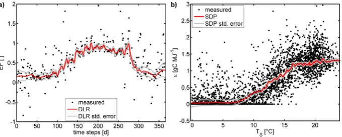
In this study, DLR is applied to estimate the evaporative fraction, EF [−], from time series of latent and sensible heat fluxes with the aim to better capture its seasonal variations and reduce the impact of short term fluctuations by noise ef-fects:

λE(t ) = EF(t )·(λE(t ) +H (t ))+ζ (t ) (2) witht being the daily time steps [d]. The sum of the latent heat flux, λE [MJ m−2d−1], and the sensible heat flux,H [MJ m−2d−1], is assumed to represent the available energy at the land surface. It shall be noted that, strictly speaking, the error seriesζ in this and all the following DLR and SDP equations has to be given a separate subscript since it is never the same error series, but in favour of a better readability and clarity we just use the symbolζ in all equations. An exam-ple for EF calculated by means of DLR is shown in Fig. 1a. Additionally, DLR is used to depict the seasonal evolution of the light use efficiency parameteras represented in: FG(t ) = (t )· APAR(t ) +ζ (t ) (3)

where FG [gC m−2d−1] is the flux of carbon uptake or

gross primary production, and APAR [MJ m−2d−1] is the ab-sorbed photosynthetically active radiation, and[gC MJ−1] is the time-varying light use efficiency parameter.

In contrast to DLR, the SDP estimation assumes that the regression parameters vary with a state of the considered non-linear system. This state variable, however, also varies with time (Young and Pedegral, 1999; Young, 2001, 2000; Young et al., 2001):

y(t ) =

n X

i=1

ci (ui(t )) ·xi(t )+ζ (t ) (4)

with ui being variables representing time-varying system

states. In the SDP algorithm,ci is again assumed to evolve

in a stochastic random walk process characterized by a white noise sequence with a zero mean. Each sample instant de-pends on the data in its vicinity in a state space in which all involved variables are sorted with respect to the state vari-ables ui, hence out of temporal order. As with the DLR

model, the NVR value determines the weighting of adjacent samples (Jarvis et al., 2004).

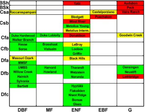
Fig. 1. (a) Example for the application of DLR to estimate the seasonal variation of the evaporative fraction, EF (see Eq. 2). Data from MMSF, 2006. (b) Example for the application of SDP to estimate the evolution of the light use efficiency () depending on the soil temperature.TS (see Eq. 3). Data from MMSF, 1999–2006.

for the data from the FLUXNET site MMSF; in this exam-ple, the dependency ofon the upper layer (2–10 cm depth) soil temperatureTS[◦C] as estimated with SDP is depicted: FG(t ) = (TS(t )) · APAR(t )+ζ (t ). (5)

For evaluation purposes of the Jarvis-model and the model formulated in this study, the Nash-Sutcliff efficiency crite-rion, EC, is applied beside the typically used coefficient of determination, r2, as squared Pearson’s correlation coeffi-cient (Legates and McCabe Jr, 1999; Krause et al., 2005), and the bias as difference of the means of measured and mod-elled time series. EC is defined as the sum of squared errors of the predicted (P) in relation to the observed (O) values normalized by the variance ofO, and subtracted from unity (Legates and McCabe Jr, 1999; Krause et al., 2005):

EC = 1 −

PN

j=1 Oj −Pj2 PN

j=1 Oj − ¯O

2 (6)

withj running from 1 to the number of observed and mod-elled time steps,N. In contrast tor2, EC is therewith sen-sitive to additive and proportional differences between mea-sured and modelled data.

To summarize the methodological approach of this study, it shall be noted again that SDP is used as a diagnostic tool to derive dependencies ofon environmental variables and therewith suitable model structures directly from the data. The outcomes of the model building study of Jarvis et al. (2004) are used as a basis to start from. The final model derived on basis of the outcome of the SDP analysis is subsequently calibrated. The parameter sensitivity is ana-lyzed within a Monte Carlo framework. Finally, the site-specifically optimized model parameters are brought into a climate-vegetation context to discuss the suitability of the model parameters for regionalization purposes.

3 Model identification

3.1 Evaluation of the Jarvis-model

Analysing daily flux data at two temperate forests (Harvard Forest, UMBS) with SDP, Jarvis et al. (2004) identified the light use efficiencyJ [gC MJ−1] with respect to FG as

ex-pressed in the following equation:

FG(t ) = J(t )·S0(t ) (7)

to follow a sigmoidal relationship with TF [◦C], the

time-delayed soil temperature (TS). In the above equation, the

above-canopy incident solar radiation (S0[MJ m−2d−1])

in-stead of the typically used absorbed PAR (APAR) was used by Jarvis et al. (2004); therefore, strictly speaking,J is not

a light use efficiency and it was therefore termed “radia-tion capture and utiliza“radia-tion coefficient” (Jarvis et al., 2004, p.940). The sigmoidal function ofJ was described by

fol-lowing equations: J(t )=

max,J

1 + exp kT,J · (TF(t )−TI)

(8) where

TF(t ) = (1 −α)· TS(t )+α ·TF(t −1). (9) TI[°C] is the inflection point ofJbetween its minimum and

maximum level (max,J [gC MJ−1]) andkT,J [◦C−1] the rate

of change of this transition. α[−] is the lag parameter for TF. The mean ofTS-values of the first 30 days was chosen

as starting point for TF. The soil temperature was filtered

because the measured time series showedmax,J responding

with delay to changes ofTS. The four parameters,max,J,TI, kT,J andα, were site-specifically calibrated by Jarvis et al.

Fig. 2. obtained by DLR (see Eq. 2) as well as modelled according to Jarvis et al. (2004), both plotted vs. the delayed soil temperature

TF. DLR is applied to estimatewith the aim to better capture seasonal variations and reduce the impact of short term fluctuations by noise effects for diagnostic purposes. Panel (a) showsof the boreal deciduous forest Sylvania Wilderness with almost no decrease offor higher temperatures, whereas (b) represents a typical example of coniferous sites (Tharandt).

broader spectrum of vegetation and climate types. To do so, the original Jarvis-model is, as a first step, run for all study sites regardless of their vegetational and climatological char-acteristics to test the suitability as well as to analyse deficien-cies of the model; the four constant model parameters (max, TI, kT andα) are optimized at each study site individually

with the non-linear least squares method with regard to the measured and modelled fluxes (FG). One difference is made

compared to Jarvis et al. (2004): For better comparability with other studies, the global radiationS0is changed to PAR,

the photosynthetically active part ofS0. This change does

not impair the model applicability of the Jarvis-model since PAR is usually a quite conservative fraction ofS0(Stigter and

Musabilha, 1982), especially on a daily basis .

The Jarvis-model reproduces well the gross CO2uptake FG of boreal and temperate forests in terms ofr2- and

EC-values with respect to the measured and modelledFG-values.

The model performs particularly well at deciduous forests with strong seasonal dynamics as Figs. 2a and 3 indicate. In the former plot, the sigmoidal function describing in the Jarvis-model is compared with the measured, which is – for better illustration of the dominant seasonal behaviour of – somewhat noise-reduced by the application of DLR (see Eq. 3).

At forests sites in warmer C-climates and at needle-leaf forests, however, the model shows deficiencies in the tem-perature dependency of: The model is not able to capture the decrease ofat high temperatures (Fig. 2b), which is not surprising considering the sigmoidal form of the function. r2- and EC-values with regard to the measured and modelled FG time series are quite satisfying for most forests, though

(Fig. 3). However, a comparison with such as shown in Fig. 2b reveals that these moderate to good model perfor-mances are often just a result of the fact that PAR itself ex-plains a large variation ofFG and, furthermore, a result of

the nature of the parameter optimization procedure, which – up to a certain degree – counterbalances shortcomings of model formulations; particularly,αseems to compensate in-appropriate model structures.FGof forest sites experiencing

hot summers as well as most grasslands cannot be simulated

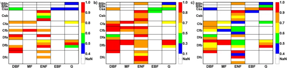
Fig. 3. Study sites in a vegetation-climate matrix; within one class, the sites are ranked according to their mean temperature from top to down. The performance of the Jarvis et al. (2004) model is in-dicated in 3 categories: good (green,r2>0.8), moderate (yellow). bad (red,r2<0.5). Koeppen-Geiger-climate classes: steppe cli-mate (BS), temperate (C), continental (D); summer dry (s), fully humid (f); hot (h), cold in winter (k); hot summer (a), warm sum-mer (b), cool sumsum-mer (c), cold winter (d); vegetation classes: de-ciduous broadleaf forest (DBF), mixed (MF), evergreen needleleaf (ENF), evergreen broadleaf (EBF), grass (G).

by the Jarvis-model at all, because the assumed sigmoidal temperature dependency ofdoes not exist, letting the con-clusion to be drawn that a water availability proxy is lacking. Even at the fully humid study sites analyzed by Jarvis et al. (2004), cross-correlations between the model residuals and a water availability measure were found. Consequently, not only the dependency oftoTS has to be reconsidered, but

Fig. 4. depending on the major driver ofFG as obtained by a SDP-model with one state variable (Eq. 4 withN= 1). State variables explainingwereTSat Duke, SWC at Vaira Ranch. API and Audubon. The grey bounds encompassing the estimated relationship represent the standard errors of the SDP estimation.

3.2 Finding new model structures

In order to identify the dominant state dependencies ofat all study sites, SDP is applied first withTS as state variable

to systematically examine which patternfollows with re-gard toTS (Eq. 5) confirming that at many sites a distinct

decrease of with increasing TS occurs (Figs. 2b and 4a).

APAR is used instead of PAR for better comparability with other studies and because of the overwhelming evidences for the significance of the LAI or FPAR as scaling-factor for soil-vegetation-atmosphere-transfer processes (Watson, 1958; Monteith, 1977; Tucker and Sellers, 1986; Goetz and Prince, 1999; Gower et al., 1999; Lindroth et al., 2008) which cannot be compensated by other environmental vari-ables used in the light use efficiency modeling approach.

At those sites where the Jarvis-model is not able to prop-erly reproduce the carbon flux dynamics at all, SDP not surprisingly also fails to find a clear temperature depen-dency which indicates some other controlling factor on the -dynamics, presumably the water availability. This failure is expressed in terms of very high standard errors of the SDP estimations and/or a lowr2-value. SDP is therefore used to analyze several water availability measures (W) as potential further controls on:

FG(t ) = (W (t ))· APAR(t )+ζ (t ) (10)

including EF (see Eq. 2), the vapor pressure deficit (VPD [kPa]), the top-layer (1–15 cm depth) soil water content (SWC [%], Fig. 4b), and the antecedent precipitation in-dex (API [mm], Fig. 4c). Besides API, these variables have demonstrated before to significantly affect gross primary production and are frequently used in light use efficiency models as moisture availability indicator (Potter et al., 1993; Prince et al., 1995; Heinsch et al., 2006; Yuan et al., 2007; M¨akel¨a et al., 2008). API is calculated by a weighted sum of daily precipitation values (P [mm]) in a time windowZ [d] before the current time stept [d] (Linsley et al., 1982; Samaniego-Eguiguren, 2003):

API(t ) =

Z X

d=0

κ−d · P (t )t−d (11)

whered denotes the number of time steps before the current stept andκ [−] is a recession constant commonly ranging between 0.85 and 0.98 (Chow, 1964). In this study, a lower boundary of 0.90 was chosen for forests and a lower bound-ary of 0.88 for grasslands; the upper boundbound-ary was retained. A cosinus function is chosen such, that κ varied between these extremes with the lowest value ofκ in summer and the highest in winter to take the higher recession of precipitation events in summer due to a higher evapotranspiration into ac-count. Indeed, in several cases the SDP-analysis shows a distinct dependency on the water availability state variables (Fig. 4b and c).

At most sites, however, neither the temperature nor a water availability proxy alone can explain the evolution oforFG,

respectively, satisfyingly. Therefore, a dimension is added to the SDP model and a two-dimensional SDP regression (see Eq. 4) is applied

FG(t ) =c1 (TS(t ))·APAR(t )+c2(W (t ))·APAR(t )+ζ (t ) (12) or respectively

FG(t ) = (c1(TS(t )) +c2(W (t ))) ·APAR(t )+ζ (t ) (13)

with

c1(TS(t )) +c2(W (t ))= (t ) (14)

usingTS and one of the mentioned water availability

prox-ies. APAR is chosen instead of S0 as used in the Jarvis

lead to somewhat higher uncertainties, i.e. the related param-eter estimations are less uniquely identifiable compared to the other state variables. The nonparametric relationship be-tweenmax andTS in the two-dimensional SDP estimation

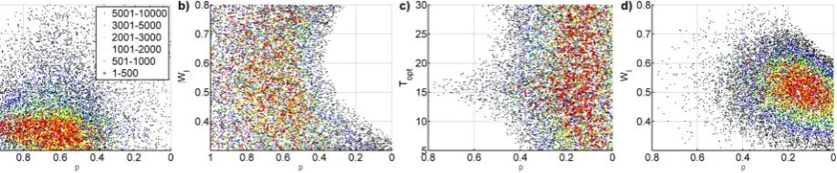
either has a sigmoidal form, or it can be described by a (sig-moidal) peak function (Fig. 5a), or no clear relationship can be identified at all (Fig. 5c). If a clear relationship between and the water availability state variable exists – as in the ma-jority of cases – it usually shows a threshold-like behaviour as demonstrated exemplarily in Fig. 5b and 5d.

3.3 Formulating the generalized model

To overcome the applicability restrictions of the basic model with the lessons learned in the SDP analysis, the sigmoid temperature function is changed to a logistic peak function, fT, which enables a decrease ofwith increasing

tempera-tures after a sigmoidal shift from the minimum to the maxi-mum level:

fT =

4 · exp − TS −Topt kT

1 + exp − TS −Topt/kT

2 (15)

withkT[◦C−1] being the rate of change andTopt[◦C] being

the temperature at which the function reaches its maximum. To allow for the effect of water availability fluctuations, a sigmoid function is used since SDP shows the tendency that at very low and very high values of the respective wa-ter availability proxiesW (EF, SWC, API and VPD) there is no change of the influence on; this behaviour is evident in the one-dimensional SDP estimation (Fig. 4b and c) and gets even more obvious when taking additively both temper-ature and moisture in one SDP-model into account (Fig. 5). The function allowing for the influence ofWonmax,fW, is

therefore chosen to be a sigmoid function: fW =

1

1 + exp (kW · (W −WI))

(16) withkWbeing the rate of change between the minimum and

maximum levels of fW and WI being the inflection point.

The units of the parameters of this subfunction depend on the variable used forW; in case of the usage of EF they are con-sequently dimensionless. BothfT as well asfWare scaled

between zero and unity.

To account for lag effects between the response of to temperature variations we allow again for the lag effect us-ing the lag-parameterαapplied toTS(Eq. 9) as it has proven

to be significant in similar light use efficiency model ap-proaches as proposed by M¨akel¨a et al. (2006, 2008) for sites in temperate and boreal climates. However, in cases ofW be-ing the main driver ofas it is the case in semi-arid climates, the lag function is applied toW instead ofTS. In applying αonly to the main driver, the number of free parameters is minimized, and the lag is anyway only apparent in a distinc-tive manner on a daily time step basis when the canopy has to

Fig. 5. as function ofTS and EF at the Mediterranean site Roc-carespampani (a, b) and as function ofTSand VPD at the desert-grassland Audubon (c, d) as determined by the additive SDP regres-sion (Eq. 12). The grey error bounds represent the standard errors of the SDP estimation.

regenerate and redevelop green tissue after a dormant period; and these periods are largely determined by the main driver such as the temperature in temperate and boreal climates and a moisture proxy in semi-arid climates.

The final model is formulated as follows:

FG =max · (p ·fT +(1 −p)· fW) · APAR (17)

wherepis a dimensionless parameter scaling the subfunc-tion to a range between zero and unity. If both temperature conditions and water availability are optimal,maxis reached.

If no humidity dependency can be detected, because there is always enough water available, and-variations can be ex-plained by the temperature,papproaches 1 and the second term approaches zero, and vice versa. 1−pis consequently indirectly a measure for the strength of the water availability influence on a vegetation stand. It is therefore an interesting site-specific parameter, particularly against the background of a subsequent model regionalization.

4 Model calibration and evaluation

The final model formulation given by Eq. (17) and its sub-funtions (Eqs. 9, 15 and 16) comprises seven constant model parameters includingmax,p,Topt,kT,WI,kW, andα.

Be-fore the final calibration, the sensitivity and variability for each of these parameters is explored. To do so, a set of 750 000 Monte Carlo simulations is executed at each loca-tion allowing the seven parameters to vary randomly within predefined (bio-physiologically meaningful) ranges follow-ing a uniform distribution. Usfollow-ing the sum of squared errors between measured and modelledFGas a performance

Fig. 6. Probability density functions (PDF) resulting from the Monte Carlo sensitivity study (N= 750 000) for the proposed model in which all seven constant model parameters could vary freely. The PDFs are drawn for the best solutions (1%) over all sites (with regard to the sum of squared errors between measured and modelledFGtime series) for the four parameters of the subfunctions (fT,fW): Topt(a),kT(b),

WI(c),kW(d). In the final model calibration,kWis set constant.

Fig. 7.fT,fWand the cumulative sums ofFGwith uncertainty bounds (grey) at Wetzstein (a) and Duke Forest (b). EF was used to model

FGin (a) and SWC in (b) as water availability measure. The 95% uncertainty bounds are due to the propagation of uncertainties in associated parameter estimates, as obtained by a Monte-Carlo simulation (N= 1000); see text for further details.

for either the parameters offTor that offW, here dependent

on the dominant control (temperature or water availability, see below). Analysing the 1% best solutions of all sites al-together reveals that the parameters leading to the best solu-tions cover a wide range within the assigned upper and lower boundaries. The respective probability distribution functions (PDF) for the seven parameters are drawn; the PDFs for the parameters of the subfunctions are depicted in Fig. 6. The PDF of the parameterkWshows the sharpest peak, thus most

of the best values at all sites are located in a relatively narrow range (Fig. 6d). Therefore, to avoid over-parameterization of the model we treated kW constant at the median of all the

bestkW-values and only the remaining six parameters,max, p,Topt,kT,WIandαare calibrated. The model calibration is

performed separately for each candidate for the water avail-ability proxyW (EF, SWC, API and VPD). The calibration is carried out using the Matlab nonlinear least-square opti-mization routine “lsqnonlin” which applies a subspace trust-region method and is based on the interior-reflective Newton method as described in Coleman and Li (1994).

The calibration performed well for all model runs:r2and EC-values of greater than 0.7 in most cases as well as rela-tively small biases indicate the ability of the model to repro-duceFG-fluxes. The parameters are generally well defined

(see Table 2). Examples offTandfWas well as the resulting

cumulative sums ofFGin comparison with measured

cumu-lative sums are shown in Fig. 7 with their 95% confidence intervals caused by the propagation of the uncertainties in the associated parameter estimates as obtained by a Monte-Carlo simulation (N= 1000); for details see e.g. Thornley and Johnson (2002). These uncertainty bounds are well bracketing measured cumulativeFG-data. The minimal and

maximal bias for all sites and models runs is −0.23 and 0.55 gC m−2_d−1_{, respectively, with positive biases occurring}

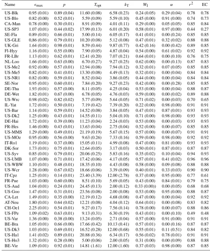
Table 2. Optimized constant model parameters with their 95% confidence intervals (in brackets) and model accuracy measures coefficient of determinationr2and efficiency criterion EC with respect to the measured and modelledFG-time series. Full site names can be found in Table 1.

Name max p Topt kT WI α r2 EC

US-Blk 0.95 (0.01) 0.89 (0.04) 11.60 (0.08) 6.58 (0.23) 0.24 (0.05) 0.29 (0.04) 0.78 0.78 US-Blo 0.82 (0.00) 0.52 (0.01) 5.59 (0.09) 5.59 (0.10) 0.45 (0.00) 0.91 (0.00) 0.74 0.73 CA-Man 0.78 (0.00) 0.30 (0.01) 8.91 (0.09) 4.01 (0.11) 0.29 (0.00) 0.05 (0.05) 0.85 0.84 US-SP3 1.07 (0.01) 0.44 (0.02) 17.99 (0.13) 6.01 (0.20) 0.58 (0.01) 0.97 (0.00) 0.44 0.27 SE-Fla 0.89 (0.01) 0.66 (0.01) 5.00 (0.14) 6.05 (0.17) 0.41 (0.01) 0.00 (0.24) 0.85 0.85 US-GLE 0,86 (0.01) 0.79 (0.01) 10.20 (0.08) 5.12 (0.08) 0.47 (0.01) 0.32 (0.02) 0.88 0.88 UK-Gri 1.64 (0.01) 0.98 (0.01) 8.59 (0.44) 9.87 (0.77) 0.42 (0.16) 0.00 (0.42) 0.89 0.85 Fl-Hyy 1.16 (0.01) 0.55 (0.00) 7.90 (0.05) 4.87 (0.04) 0.54 (0.00) 0.61 (0.02) 0.92 0.92 FR-LBr 1.13 (0.01) 0.62 (0.01) 12.41 (0.20) 7.07 (0.21) 0.64 (0.01) 0.00 (0.10) 0.76 0.75 NL-Loo 1.66 (0.01) 0.63 (0.00) 6.70 (0.27) 9.27 (0.25) 0.62 (0.00) 0.00 (0.13) 0.87 0.83 US-Me2 0.92 (0.00) 0.57 (0.01) 12.94 (0.08) 7.94 (0.12) 0.32 (0.01) 0.07 (0.05) 0.85 0.85 US-Me5 0.82 (0.01) 0.41 (0.01) 13.30 (0.08) 4.49 (0.13) 0.32 (0.01) 0.00 (0.04) 0.84 0.84 US-NR1 0.82 (0.00) 0.59 (0.01) 8.52 (0.04) 3.86 (0.05) 0.44 (0.00) 0.00 (0.04) 0.84 0.84 SE-Nor 0.95 (0.01) 0.60 (0.01) 7.84 (0.20) 9,27 (0.23) 0.42 (0.00) 0.00 (0.28) 0.85 0.85 DE-Tha 1.93 (0.01) 0.57 (0.00) 8.11 (0.05) 4.25 (0.04) 0.53 (0.00) 0.00 (0.04) 0.88 0.87 DE-Wet 1.82 (0.01) 0.67 (0.00) 6.78 (0.05) 4.76 (0.03) 0.59 (0.00) 0.00 (0.02) 0.89 0.88 US-Wrc 0.98 (0.02) 0.82 (0.02) 5.77 (0.09) 5.64 (0.05) 0.71 (0.02) 0.00 (0.03) 0.70 0.65 IL-Yat 1.72 (0.01) 0.50 (0.01) 7.19 (0.42) 7.39 (0.20) 0.22 (0.00) 0.98 (0.00) 0.91 0.91 US-Bar 1.14 (0.01) 0.59 (0.01) 14.52 (0.08) 3.84 (0.05) 0.47 (0.01) 0.87 (0.01) 0.93 0.93 US-Dk2 1.25 (0.00) 0.43 (0.01) 14.55 (0.11) 5.04 (0.10) 0.71 (0.00) 0.98 (0.00) 0.93 0.93 DE-Hai 1.72 (0.01) 0.39 (0.00) 11.23 (0.04) 2.24 (0.03) 0.53 (0.00) 0.00 (0.03) 0.93 0.93 FR-Hes 1.46 (0.00) 0.43 (0.01) 13.63 (0.04) 2.75 (0.04) 0.52 (0.00) 0.00 (0.07) 0.85 0.85 US-MMS 1.29 (0.00) 0.49 (0.01) 21.19 (0.19) 5.67 (0.15) 0.57 (0.00) 0.00 (0.07) 0.91 0.91 US-MOz 0.95 (0.00) 0.56 (0.00) 9.63 (0.26) 7.33 (0.16) 0.59 (0.00) 0.98 (0.00) 0.92 0.92 IT-Ro1 1.19 (0.01) 0.37 (0.00) 15.05 (0.11) 4.99 (0.08) 0.47 (0.00) 0.81 (0.00) 0.93 0.93 DK-Sor 1.73 (0.01) 0.75 (0.01) 12.64 (0.05) 3.17 (0.03) 0.50 (0.01) 0.87 (0.01) 0.87 0.87 US-Syv 0.85 (0.01) 0.79 (0.01) 20.06 (0.25) 5.83 (0.16) 0.35 (0.02) 0.10 (0.04) 0.94 0.93 US-UMB 1.07 (0.00) 0.71 (0.01) 17.42 (0.06) 4.17 (0.05) 0.57 (0.01) 0.41 (0.02) 0.96 0.96 US-WBW 1.10 (0.01) 0.48 (0.01) 18.35 (0.10) 4.43 (0.08) 0.58 (0.00) 0.09 (0.08) 0.88 0.88 US-Wcr 1.28 (0.00) 0.67 (0.02) 18.66 (0.06) 3.39 (0.09) 0.40 (0.01) 0.33 (0.03) 0.90 0.90 IT-Cpz 1.25 (0.01) 0.14 (0.01) 23.40 (3.39) 12.00 (2.78) 0.37 (0.00) 0.95 (0.00) 0.77 0.61 FR-Pue 1.03 (0.00) 0.60 (0.00) 8.51 (0.10) 5.69 (0.05) 0.43 (0.00) 0.84 (0.01) 0.79 0.75 US-Aud 1.04 (0.01) 0.24 (0.01) 24.45 (0.13) 2.00 (0.12) 0.33 (0.00)) 0.00 (0.05) 0.68 0.68 US-Goo 1.47 (0.01) 0.31 (0.01) 23.56 (0.08) 2.00 (0.08) 0.53 (0.00) 0.95 (0.00) 0.88 0.87 CA-Let 1.49 (0.01) 0.35 (0.00) 12.19 (0.12) 4.68 (0.08) 0.47 (0.00) 0.00 (0.04) 0.92 0.92 AT-Neu 1.80 (0.01) 0.64 (0.02) 12.21 (0.08) 4.04 (0.12) 0.64 (0.01) 0.00 (0.08) 0.83 0.82 CH-Oe1 2.25 (0.01) 0.54 (0.01) 9.27 (0.17) 7.56 (0.14) 0.78 (0.00) 0.00 (0.07) 0.88 0.86 US-FPe 1.09 (0.02) 0.63 (0.01) 9.13 (0.31) 6.30 (0.19) 0.43 (0.01) 0.00 (0.10) 0.49 0.48 US-Var 1.36 (0.00) 0.38 (0.00) 13.24 (0.05) 2.71 (0.04) 0.57 (0.00) 0.91 (0.00) 0.91 0.91 BE-Bra 1.05 (0.01) 0.66 (0.00) 17.66 (0.42) 10.13 (0.41) 0.57 (0.01) 0.00 (0.16) 0.87 0.87 US-Dk3 1.03 (0.01) 0.69 (0.01) 16.52 (0.28) 12.00 (0.68) 0.55 (0.01) 0.11 (0.51) 0.84 0.82 US-Ha1 1.41 (0.02) 0.89 (0.01) 20.88 (0.36) 6.34 (0.17) 0.56 (0.02) 0.78 (0.01) 0.91 0.91 US-Ho3 1.32 (0.01) 0.28 (0.00) 5.00 (0.06) 2.00 (0.05) 0.31 (0.00) 0.00 (0.09) 0.88 0.88 BE-Vie 1.09 (0.01) 0.92 (0.01) 14.81 (1.61) 12.00 (1.60) 0.37 (0.03) 0.98 (0.00) 0.87 0.85

In the following, results are described in more detail for the model with EF instead of SWC, API and VPD as water availability proxy, since (i) the calibrations with EF resulted in the highest quality criteria with generally the lowest confi-dence intervals, (ii) overall, EF already performed best in the

Fig. 8. The six model parametersmax(a),p(b),Topt(c),kT (d),WI(e),α(f) in a vegetation and climate context. See Fig. 3 for an explanation of the abbreviations.

there is the potential it can be retrieved by remote sensing (Crago, 1996). Results for the other moisture surrogates are shown exemplarily (Figs. 7b and 11). The resulting parame-ters of the optimization procedure, their confidence intervals, r2-values and model efficiencies EC are given in Table 2 for the EF-model. All calibrated constant model parameters are shown in a climate-vegetation-matrix (Fig. 8).

The parameters offThave in general wider confidence

in-tervals thanWI of fW; one reason for this certainly is the

fact thatfThas two free parameters, another reason can be

found in the wider range of temperature values compared to EF. However, fixation of one parameter of fT deteriorates

the model performance too much. The higher p, thus the more the temperature dominates the variations ofFG, and

the smaller the confidence intervals of the parameterskTand Topt of the corresponding temperature function tend to be.

Even more pronounced is the effect vice versa: The smaller p, thus the higher the influence of EF, the smaller are the con-fidence intervals ofWIby trend (Fig. 9a). This fact can also

be seen in the SSE-values resulting from a Monte Carlo sen-sitivity study. This was performed again for the final model with the six free model parameters: For highp-values, thus a high influence of the temperature onFG, theTopt-values of

the best parameter sets are typically located in a relatively narrow range, and vice versa, ifpis low and EF dominates FGvariations,WIis usually better defined (Fig. 10). This

ob-served characteristic is an advantage of the proposed model structure: the model is on the one hand flexible enough to

Fig. 9. 95% confidence intervals of the calibrated model parameters

Fig. 10. The parameter space ofpandTopt(a, c) andpandWI(b, d) resulting from Monte Carlo simulations (10 000 best parameter sets according to the sum of squared errors (SSE) between measured and modelledFG-values out of 750 000 runs) showsToptbeing well defined ifpis high (greater contribution offT) as shown for Wetzstein (a) andWIbeing better defined ifpis low (greater contribution offW) such as at Lethbridge (d). The same is true vice versa:WIis not well defined iffThas the greater contribution such as at Wetzstein (b). andTopt is rather insensitive iffWdominates such as at Lethbridge (c). The colors represent different classes with regard to the sorted SSE-values; the numbers refer to the ranking of the model results with regard to these values.

simulate daily fluxes of sites with very different characteris-tics, but on the other hand, gives less weight to the less influ-encing variables, which are at the same time prone to uncer-tainties in model parameter optimizations. From Fig. 9b it is also obvious that with increasing length of the calibration time series the parameter confidence intervals tend to narrow, hence better results can be expected with the availability of longer measurement time series.

The model parameter max varied at forest sites

be-tween 0.78 gC MJ−1 _{at a needleleaf forest in Canada and}

1.93 gC MJ−1 at a German needleleaf forest in a temperate climate with mild summers (Cfc). Deciduous forests form the highest averagemaxwith a mean of 1.25 gC MJ−1

fol-lowed by the mixed forests (1.18 gC MJ−1) and evergreen needleleaf forests (1.16 gC MJ−1). Evergreen broadleaf forests have with 1.14 gC MJ−1the lowest averagemaxdue

to low values in boreal climates and those with dry summers. Regarding the climate classes with more than one forest site, Cfb-class reveals the highest averagemax, closely followed

by Dfb; Csb and Dfc have the lowestmax. At grasslands

sites, max-values are surprisingly high: max-estimations

reach 2.25 at Oensingen and 1.80 at Neustift and lead to an averagemaxof 1.50 gC MJ−1. The highest max-values at

Oensingen are attained in spring and autumn when tempera-tures are favourable but the amount of incoming radiation is still relatively low.

Optimized parameter values for p, indicating the influ-ence ofTS and EF, range between zero and unity and only

the lowest values are omitted:FGat the Mediterranean

Roc-carespampani and at Audubon, Arizona, is largely explained by EF with ap-value of 0.14 and 0.24, respectively,FG at

Griffin, England, follows highly the course of temperature (p= 0.98). Most forest sites, however, have a medium p -value between 0.4 and 0.8. The lowp-values at Hainich and especially at Boreas and Howland can be explained by a an especially high correlation betweenand EF in the seasonal course. At Hainich, particularly the distinct summer drought of 2003 (Reichstein et al., 2007) with a strong decrease of

in late summer leads to an higher influence than at the other sites in this climate class. p-values greater than 0.6 are mainly clustered in the forest and fully humid climate classes, whereasp-estimates at forests at summery sites as well as grasslands take values in the medium to lower range. The temperature Topt at which the sites reach max is

smaller than 14◦C for the all needleleaf forests but the warmest fully humid study site, a result of lower average temperatures and high light use efficiencies in spring and autumn. The deciduous forests, instead, have Topt-values

greater than 14◦C; here, the most efficient periods occur when the leafs have emerged following the rise of temper-ature in spring and before the loss of the leafs or they occur even in summer when temperatures get not too high and there is no lack of water. The grasslands located at sites with hot and semi-arid conditions are dominated by medium to high Topt-values up to 24.5◦C in case humid and warm periods

coincide. The alpine and northern Dfb grassland sites are characterized by medium to lowTopt-estimates

correspond-ing to the mild average temperatures and highest efficiencies in spring and autumn.

In addition to the information at which temperaturemax

occurs, the parameterkT characterizes the steepness of the

temperature sensitivity in relation to the temperature range and the vegetation period. Accordingly, deciduous forests, especially at colder sites, as well as grasslands at semi-arid sites have rather low kT-values corresponding to a sharper

peak of the temperature function, whereas evergreen sites particularly with a relatively small annual temperature range feature medium to high kT-values leading to a flatter and

wider peak.

The parameterWIdetermining the inflection point of the fW-function takes in the most cases values between 0.3

and 0.7, but more extreme values are represented, too. The lower WI-values cluster in the cooler climate classes and

those with hot and dry summers, whereas the representatives of the upper third of theWI-range cluster in the fully humid

Fig. 11. Model parameterpwith respect to vegetation and climate classes for the model runs with SWC (a), API (b), and VPD (c) as input variables. See Fig. 3 for an explanation of the abbreviations.

The optimized values of model parameterα, finally, are assigned to one end of the scale between zero and unity in most cases. It reaches high values near unity reflecting dis-tinct lag processes at deciduous study sites throughout the climate classes and warmer sites of the other forest classes. However, in the most classes both extremes – lag effects and direct correspondence of α and the state variable, are rep-resented. The C-climate grasslands show delay processes whereas the grasslands in semi-arid and hot as well as con-tinental D-climates seem to react rather promptly to the trig-gering variables.

Finally, the parameterpfor the further water availability proxies SWC, API and VPD is presented in Fig. 11. In case of SWC and API it illustrates a more homogeneous pattern of p-values within the vegetation-climate-matrix with lowerp -values predominating in B- and summery climates as well as grasslands with exception of the alpine sites. More often than for SWC and API, a higher explaining power is attributed to VPD, especially at warmer coniferous sites. The highest influence of aW substitute, however, is assigned to API at the desert grassland Audubon with ap-value of 0.15, thus a contribution of 85%.

5 Discussion

State dependent parameter estimation was used to deter-mine typical non-parametric relationships between the light use efficiency and relevant state variables. An one and two-dimensional SDP estimation revealed the relationship between and TS to follow a (sigmoidal) peak function.

Limiting functions with respect to temperature have been used before: E.g. M¨akel¨a et al. (2008) tested a model at several coniferous study sites and used a site-specific piece-wise function with a linearly increasing part and a constant value above a threshold temperature; this approach con-trasts with this study, in which especially the coniferous for-est sites show a relatively small efficiency amplitude during the year with the highest -efficiencies at lower tempera-tures followed by an efficiency-decrease at higher temper-atures. Yuan et al. (2007) who also modelledFG across a

broad range of conditions applied a peak function, too. They estimated the temperature optimum by non-linear optimiza-tion merging the data from all study sites. In our study, however, it is shown that highest efficiencies occur at tem-peratures that vary significantly across study sites. Regard-ing moisture availability measures, various functional forms as well as different proxies have been applied previously: E.g., Yuan et al. (2007) chose a linear relationship between and EF. M¨akel¨a et al. (2008) represented the relationship betweenand VPD by an exponential function and between and SWC by a Weibull-function or a sigmoidal function following Landsberg and Waring (1997). In this study, SDP revealed in most cases a threshold-like response of to all proxies givenwas sensitive to them. Overall, SDP showed a combination of the temperature and a water availability measure to be an appropriate way to modelFG if the

studies (e.g. Yuan et al., 2007, 2010), this approach is based on the assumption that no universal maximum and opti-mal temperature exist even under ideal conditions; we as-sume, instead, that biochemical processes are not universal across species and that maximum-values, optimal temper-atures and other parameters vary between vegetation stands (Turner et al., 2003; Bradford et al., 2005; Schwalm et al., 2006; Kjelgaard et al., 2008; Stoy et al., 2008). Predictions with this model approach obviously require sufficiently long measurement time series covering optimal periods for vege-tation growth. The minimum required measurement period of three years presupposed in this study can be critical in this sense (Nouvellon et al., 2000). But this restriction will become less important when FLUXNET measurement time series get longer and are made available for such calibration studies.

With the data available the calibrated parametermax

var-ied strongly between sites as expected for the reasons stated above. Compared to maximum light use efficiency val-ues of several studies reported in the comprehensive litera-ture review of Goetz and Prince (1999) the calibrated val-ues from this study appear to be somewhat greater. Com-pared to the average values per vegetation type obtained by Garbulsky et al. (2010) from measurement data, however, the max-values tend to be smaller; the highestmax-value

in their study was 2.01 gC MJ−1 compared to a value of 2.25 gC MJ−1 in our study. However, in both studies most vegetation types were statistically not representative; and certainly, they are significantly influenced by the choice of the FPAR data source and the processing of the measured or remotely sensed data. Interestingly, the highestmax-value

reached at the grassland Oensingen is equal to the globally calibrated potential light use efficiency in the modeling study of Yuan et al. (2010). On basis of eddy-covariance data, Gar-bulsky et al. (2010) determined also grasslands as vegetation type with the highestmax-values among their 35 study sites.

The highest forestmaxis found at Tharandt; in their

model-ing study, M¨akel¨a et al. (2008) observed a high potentialmax

at Tharandt relative to other study sites, too.

The calibration of p shows that temperature has indeed a high influence on, especially in cooler ecosystems, as shown by numerous studies (Runyon et al., 1994; Chen et al., 1999; Nouvellon et al., 2000; Turner et al., 2003; Schwalm et al., 2006). SWC as modulating variable had the highest impact at summerdry sites and grasslands what is not surpris-ing considersurpris-ing the short rootsurpris-ing depth and the low depth at which the SWC-measurements were made. VPD appears to influencenot only in dry areas aspvalues around 0.6 in bo-real and temperate forests indicate; indeed, the interrelation between VPD andvia stomatal conductance has often been shown (Wang and Leuning, 1998; Goetz and Prince, 1999; Lagergren et al., 2005; Katul et al., 2003; McCaughey et al., 2006) which contrasts with the study of Garbulsky et al. (2010) who only found a weak influence of VPD. Model runs with API do not reach the performance of the other model

configurations, but at sites with strong periodic water short-age they can explain-variations with the lowestp-values, thus the highest contribution of allfW-functions compared

to the other W-variables. API is therefore considered as promising variable. Overall, however, the optimization pro-cedure assigns EF most often the highest explaining capa-bility on, and model runs with EF lead to the best results. This is not surprising considering the observed correlation of and EF (Monteith and Greenwood, 1986; Schulz and Jarvis, 2004) and thus EF being an “integrator” of environ-mental conditions. The model with EF consequently leads to a somewhat better model performance and even allows the modeling of managed sites such as Oensingen and Neustift to a certain degree. This behaviour is supported by Stoy et al. (2009) who performed a orthonormal wavelet transformation analysis on measured CO2-fluxes and found a high

impor-tance of “endogenous” variables compared to purely mete-orological variables and a strong coupling betweenλE and FG. In the analysis of Garbulsky et al. (2010), EF is also

determined to be the best explaining variable of. In their study, EF alone explainedbest and their model deteriorated when adding another variable. This contradicts with our SDP analysis and final model calibration which assigned EF a sig-nificant influence but never the only contribution to the vari-ation of:p-values of nearly unity occurred but only in one case ap-value of smaller than 0.2 was determined. Overall, both SDP-analysis and the model application show that both temperature and water availability influence the variation of but can not explained by one variable alone.

Throwing a glance at the distribution of the other model parameters in the climate-vegetation matrix may lead to the assumption that the optimized parameter values have no bearing on site specific characteristics. However, in the ma-jority of cases the parameter values can be related to the veg-etation class (i.e. deciduous or evergreen), the length of the vegetation period (higher or lowerkT), the season in which gets maximal, the seasonal fluctuation of LAI and the de-gree of its minimization in dormant periods, the start of the vegetation period in relation to the course of temperature, the temperature amplitude, or the degree of superposition of sea-sonal temperature and humidity course. Noticeable are for example the differences of such similar forest sites as How-land and Harvard; both are located in the same category in the climate-vegetation matrix: mixed forests in a boreal climate with warm summers. While the mean annual temperature is somewhat lower at Harvard, maximum-values at Howland occur in spring and autumn whereas the maximumat Har-vard occurs rather in summer which explains the higherTopt

indicating a higher fraction of deciduous trees than at How-land; the higherat Harvard is in line with the assumptions that Harvard needs more time to develop foliage and reach max.

2006; Jenkins et al., 2007).

6 Conclusions

A parsimonious light use efficiency model has been set up on the basis of findings from state dependent parameter es-timations. It follows the assumption that the seasonal be-haviour of canopies varies between vegetation classes and its environmental conditions and the influence of explain-ing variables differs. It is hence assumed that no universal parameter set explaining the variation of CO2uptake of all

vegetation types in every climate class exists. The derived model is driven by incoming photosynthetically active ra-diation, its fraction absorbed by vegetation, the temperature and a moisture availability measure such as the evaporative fraction, the antecedent precipitation index, vapour pressure deficit or the soil moisture. Despite its simplicity it seems to capture a major proportion of the day-to-day variations in the gross CO2 uptake at 44 FLUXNET sites with largely well

defined parameters. Obviously, due to its empirical nature the parameter sets will get more robust, the longer available time series are. The best agreement between model and ob-servations are obtained using the evaporative fraction since this variable appears to incorporate more information than purely water availability. The proposed model uses variables which can be derived by remote sensing or taken from re-analysis databases like ERA-Interim from ECMWF or data from the NASA Data Assimilation Office (DAO). Addition-ally, the model parameters can be related to the specific en-vironmental conditions which lead us to the conclusion that the model is suitable as basis for regionalization strategies to perform the step from the point to the area.

Acknowledgements. We gratefully acknowledge all FLUXNET

in-vestigators generously providing level 2 data for this analysis. Specifically, we thank:

– Christof Ammann of the Swiss Federal Research Station ART, Z¨urich, for data of Oensingen,

– Marc Aubinet of the Universitaire des Sciences Agronomiques for data of Vielsalm.

– Dennis Baldocchi of the University of California, Berkeley, for data of Vaira Ranch,

– Paul Berbigier of INRA-Bioclimatology for data of Le Bray,

– Christian Bernhofer of the TU Dresden for data of Tharandt,

– Ken Bible of the University of Washington for data of the Wind River Canopy Crane Research Facility,

University of Antwerp, for data of Brasshaat,

– Peter S. Curtis of The Ohio State University for data of Uni-versity of Michigan Biological Station (UMBS),

– Danilo Dragoni and HaPe Schmid of the Indiana University, funded by the US Department of Energy Terrestrial Carbon Processes program (DOE TCP), for data of Morgan Monroe State Forest (MMSF),

– Lawrence B. Flanagan of the University of Lethbridge for data of Lethbridge,

– Allen H. Goldstein of the University of California, Berkeley, for data of Blodgett,

– Andre Granier of the French National Institute for Agricultural Research for data of Hesse,

– Lianhong Gu of the Oak Ridge National Laboratory for data of Missouri Ozark,

– David Y. Hollinger of the US Forest Service for data of How-land Forest,

– Gabriel G. Katul of Duke University for data of Duke Forest (Loblolly Pine),

– Werner L. Kutsch of Max-Planck-Institute for Biogeochem-istry at Jena (now at: the German Federal Research Institute for Rural Areas, Forestry and Fisheries) for data of Hainich,

– Beverly E. Law of Oregon State University for data of Metolius funded by DOE Grant no. DE-FG02-06ER64318,

– Anders Lindroth of Lund University for data of Flakaliden and Norunda,

– Timothy A. Martin of the University of Florida for data of Don-aldson,

– William J. Massman of US Forest Service for data of Glees,

– Tilden Meyers of NOAA for data of the study sites Black Hills, Walker Branch, Audubon, Goodwin Creek, Peck,

– John B. Moncrieff and R. J. Clement of the School of Geo-Sciences, The University of Edinburgh, as part of the CarboEu-rope programme for data of Griffin,

– Russell Monson of the University of Colorado for Niwot Ridge,

– Eddy J. Moors of Wageningen University for data of Loobos,

– J. William Munger of Harvard University for data of Harvard Forest,

– Ram Oren, Paul Stoy, Gaby Katul, Kim Novick, Mario Siqueira and Jehnyih Juang of Duke University for data of Duke Forest (Hardwood),

– Serge Rambal of CEFE-CNRS for data of Puechabon,

– Corinna Rebmann of the Max-Planck-Institute for Biogeo-chemistry at Jena for data of Wetzstein,

– Andrew D. Richardson of Harvard University for data of Bartlett,

– Riccardo Valentini of the University of Tuscia for data of Roc-carespampani, Castelporziano,

– Timo Vesala of the University of Helsinki for data of Hyyti¨al¨a,

– Steve Wofsy from Harvard University (1994–2005) and Brian Amiro from University of Manitoba (2005–2008) for data of Boreas,

– Dan Yakir of the Weizmann Institute of Science for data of Yatir, Israel,

We appreciate the comments of Christof Ammann and Ankur Desai on the manuscript. The data were downloaded from the Car-boEuropeIP Ecosystem Component Database supported by the European Commission, as well as from the AmeriFlux data archive at the Carbon Dioxide Information Analysis Center (CDIAC) of DOE’s (US Department of Energy) Oak Ridge National Laboratory (ORNL). This study was funded by the Deutsche Forschungsge-meinschaft (DFG, Grant #SCHU1271/4-1).

Edited by: R. Duursma

References

Acevedo, O., Moraes, O., Degrazia, G., Fitzjarrald, D., Manzi, A., and Campos, J.: Is friction velocity the most appropriate scale for correcting nocturnal carbon dioxide fluxes?, Agr. Forest Me-teorol., 149, 1–10, 2009.

Allard, V., Ourcival, J. M., Rambal, S., Joffre, R., and Ro-cheteau, A.: Seasonal and annual variation of carbon ex-change in an evergreen Mediterranean forest in southern France, Global Change Biol., 14, 714–725, doi:10.1111/j.1365-2486.2008.01539.x, 2008.

Ammann, C., Spirig, C., Leifeld, J., and Neftel, A.: Assess-ment of the nitrogen and carbon budget of two managed tem-perate grassland fields, Agr. Ecosyst. Environ., 133, 150–162, doi:10.1016/j.agee.2009.05.006, 2009.

Anthoni, P., Unsworth, M., Law, B., Irvine, J., Baldocchi, D., Tuyl, S., and Moore, D.: Seasonal differences in carbon and water va-por exchange in young and old-growth ponderosa pine ecosys-tems, Agr. Forest Meteorol. 111, 203–222, doi:10.1016/S0168-1923(02)00021-7, 2002.

Aubinet, M., Chermanne, B., Vandenhaute, M., Longdoz, B., Yer-naux, M., and Laitat, E.: Long term carbon dioxide exchange above a mixed forest in the Belgian Ardennes, Agr. Forest Meteorol., 108, 293–315, doi:10.1016/S0168-1923(01)00244-1, 2001.

Baldocchi, D., Falge, E., Gu, L. H., Olson, R., Hollinger, D., Running, S., Anthoni, P., Bernhofer, C., Davis, K., Evans, R., Fuentes, J., Goldstein, A., Katul, G., Law, B., Lee, X. H., Malhi, Y., Meyers, T., Munger, W., Oechel, W. U. K. T. P., Pilegaard, K., Schmid, H. P., Valentini, R., Verma, S., Vesala, T., Wilson, K., and Wofsy, S.: FLUXNET: A new tool to study the tem-poral and spatial variability of ecosystem-scale carbon dioxide,

water vapor, and energy flux densities, B. Am. Meteorol. Soc., 82, 2415–2434, 2001.

Barr, A. G., Black, T. A., Hogg, E. H., Griffis, T. J., Morgenstern, K., Kljun, N., Theede, A., and Nesic, Z.: Climatic controls on the carbon and water balances of a boreal aspen forest, 1994– 2003, Global Change Biol., 13, 561–576, doi:10.1111/j.1365-2486.2006.01220.x, 2007.

Berbigier, P., Bonnefond, J., and Mellmann, P.: CO2 and water vapour fluxes for 2 years above Euroflux forest site, Agr. Forest Meteorol., 108, 183–197, doi:10.1016/S0168-1923(01)00240-4, 2001.

Beven, K. and Freer, J.: Equifinality, data assimilation, and uncer-tainty estimation in mechanistic modelling of complex environ-mental systems using the GLUE methodology, J. Hydrol., 249, 11–29, doi:10.1016/S0022-1694(01)00421-8, 2001.

Bradford, J., Hicke, J., and Lauenroth, W.: The relative impor-tance of light-use efficiency modifications from environmen-tal conditions and cultivation for estimation of large-scale net primary productivity, Remote Sens. Environ., 96, 246–255, doi:0.1016/j.rse.2005.02.013, 2005.

Carrara, A., Kowalski, A., Neirynck, J., Janssens, I., Yuste, J., and Ceulemans, R.: Net ecosystem CO2exchange of mixed forest in Belgium over 5 years, Agr. Forest Meteorol., 119, 209–227, doi:10.1016/S0168-1923(03)00120-5, 2003.

Carrara, A., Janssens, I., Curiel Yuste, J., and Ceulemans, R.: Seasonal changes in photosynthesis, respiration and NEE of a mixed temperate forest, Agr. Forest Meteorol., 126, 15–31, doi:10.1016/j.agrformet.2004.05.002, 2004.

Chen, W., Black, T., Yang, P., Barr, A., Neumann, H., Nesic, Z., Blanken, P., Novak, M., Eley, J., Ketler, R., and Cuency, A.: Effects of climatic variability on the annual carbon sequestra-tion by a boreal aspen forest, Global Change Biol., 5, 41–53, doi:10.1046/j.1365-2486.1998.00201.x, 1999.

Chow, V. T.: Handbook of applied hydrology, McGraw-Hill, New York, 1964.

Clement, R., Moncrieff, J., and Jarvis, P.: Net carbon productivity of Sitka spruce forest in Scotland, Scottish Forestry, 57, 5–10, 2003.

Coleman, T. and Li, Y.: On the convergence of reflective New-ton methods for large-scale nonlinear minimization subject to bounds, Math. Programm., 76, 189–224, 1994.

Collatz, G., Ball, J., Grivet, C., and Berry, J.: Physiological and environmental regulation of stomatal conductance, photosynthe-sis and transpiration: a model that includes a laminar boundary layer, Agr. Forest Meteorol., 54, 107–136, doi:10.1016/0168-1923(91)90002-8, 1991.

Cook, B., Davis, K., Wang, W., Desai, A., Berger, B., Teclaw, R., Martin, J., Bolstad, P., Bakwin, P., Yi, C., and Heilman, W.: Carbon exchange and venting anomalies in an upland deciduous forest in northern Wisconsin, USA, Agr. Forest Meteorol., 126, 271–295, doi:10.1016/j.agrformet.2004.06.008, 2004.

Coops, N. C., Waring, R. H., and Law, B. E.: Assessing the past and future distribution and productivity of ponderosa pine in the Pacific Northwest using a process model, 3-PG, Ecol. Modell., 183, 107–124, doi:10.1016/j.ecolmodel.2004.08.002, 2005. Cox, P., Betts, R., Jones, C., Spall, S., and Totterdell, I.: