South African Financial Markets

(1)

South African Financial Markets

Graeme West

Financial Modelling Agency

graeme@ﬁnmod.co.za

(2)

I would like to thank

• The 2003 Wits class for useful comments and corrections, in particular Nevena Selic for clari-ﬁcation of some statistical issues.

• Dr Jaco van der Walt of Rand Merchant Bank, attendee of the 2004 Wits class, for numerous very helpful comments. Likewise the 2004 UCT class, for superb high quality feedback.

• Dr Jaco van der Walt for writing much of, and Dr Johan van den Heever of the SARB for contributions to, Chapter2.

Financial Modelling Agency is the name of the author’s consultancy. He is available for training on, consulting on and building of financial models, of both a derivative and a risk measurement nature. This is a course which attempts to apply the theory of finance to the unique features of South African markets. So, for example, we completely avoid foreign exchange markets, as the practice globally is standardised. The South African market is characterised by subtly different formulae, and sparse data. So we will see that practice can be a long way from theory:

The experimentalist comes running excitedly into the theorist’s office, waving a graph taken off his latest experiment. “Hmmm,” says the theorist, “That’s exactly where you’d expect to see that peak. Here’s the reason.” A long logical explanation follows. In the middle of it, the experimentalist says “Wait a minute”, studies the chart for a second, and says, “Oops, this is upside down.” He fixes it. “Hmmm,” says the theorist, “you’d expect to see a dip in exactly that position. Here’s the reason...”.

Nevertheless, one can be precise, and such precision has its rewards in being able to be more than a na¨ıve user of systems:

(3)

The time value of money

1.1 Discount and capitalisation functions

The owner of funds charges a fee, known as interest, for the usage of funds. Thus future values are more than present values; present values are less than future values. We have two functions

𝐶(𝑡, 𝑇) (1.1)

the capitalisation function, denoting the amount that needs to be paid at time𝑇 in return for usage of 1 in the time [𝑡, 𝑇]; and

𝑍(𝑡, 𝑇) (1.2)

the present value function, denoting the amount that needs to be handed over at time𝑡 and used in time [𝑡, 𝑇] in return for repayment of 1 at time 𝑇.1

Note that

𝑍(𝑡, 𝑇) = 1

𝐶(𝑡, 𝑇) (1.3)

and𝑍(𝑡, 𝑡) = 1 =𝐶(𝑡, 𝑡);𝑍(𝑡, 𝑇) is decreasing, with𝑍(𝑡, 𝑇)→0 as𝑇 → ∞.

A fundamental result in Mathematics of Finance is (intuitively) that the value of any instrument is the present value of it’s expected cash ﬂows. So the present value function is important.

Time is measured in years, with the current time typically being 0. So, in this notation, one might rather write𝑍(0, 𝑇) or𝐶(0, 𝑇) if it is understood without doubt when now is.

Example 1.1.1. Can pay 103 in 3 months or 113 in 1 year for use of 100 now.

𝐶(0,₁₂3) = 1.03,𝐶(0,1) = 1.13.

1.2 Compounding rates

Example 1.2.1. I can receive 12.5% at the end of the year, or 3% at the end of each 3 months for a year. Which option is preferable?

1_{Also denoted}_𝐵₍_{𝑡, 𝑇}_{) (B for bond) or}_𝐷₍_{𝑡, 𝑇}_{) (D for discount) in some sources. Our}_𝑍_{represents zero, for zero}

(9)

Option 1: receive 112.5% at end of year. So 𝐶(0,1) = 1.125. We say: we earn 12.5% NACA (Nominal Annual Compounded Annually)

Option 2: receive 3% at end of 3, 6 and 9 months, 103% at end of year. We say: we earn 12% NACQ (Nominal Annual Compounded Quarterly). Then𝐶(0,1) = 1.034_{= 1}_.₁₂₅₅_..._{, so this option}

is preferable.

This introduces the idea of compounding frequency. We have NAC* rates (* = A, S, Q, M, W, D) as well as simple rates. Note that

A annual standard S semi-annual bonds

Q quarterly JIBAR, LIBOR M monthly call rate, credit cards W weekly carry market

D daily overnight rates

Example 1.2.2. I earn 10% NACA for 5 years. The money earned by time 5 is (1 + 10%)5 = 1.610510.

Example 1.2.3. I earn 10% NACQ for 5 years. The money earned by time 5 is (1 +10%₄ )

4⋅5

= 1.638616.

Example 1.2.4. I earn 10% NACD for 5 years. The money earned by time 5 is(1 +10%₃₆₅)

365⋅5

= 1.648608.

What do we do about leap years? We’ll come to this later.

There is no such calculation for weeks. There are NOT 52 weeks in a year. If𝑟is the rate of interest NAC𝑛, then at the end of one year we have(

1 + 𝑟 𝑛

)𝑛

, in general

𝐶(𝑡, 𝑇) =(1 + 𝑟

𝑛

)𝑛(𝑇−𝑡)

We always assume that the cash is being reinvested as it is earned. Now, the sequence (1 +_𝑛𝑟)𝑛 (for𝑟 ﬁxed) is increasing in 𝑛, so if we are to earn a certain numerical rate of interest, we would prefer compounding to occur as often as possible. The continuous rate NACC is actually the limit of discrete rates:

𝑒𝑟= lim 𝑛→∞

(

1 + 𝑟

𝑛

)𝑛

(1.4)

Thus the best possible option is, for some ﬁxed rate of interest, to earn it NACC.

The assumption will always be that, in determining equivalent rates, repayments are reinvested. This implies that for the purpose of these equivalency calculations,

𝐶(𝑡, 𝑇) =𝐶(𝑡, 𝑡+ 1)𝑇−𝑡 (1.5) Example 1.2.5. The annual rate of interest is 12% NACA. Then the six month capitalisation factor (in the absence of any other information) is√1.12.

If𝑟(𝑛) denotes a NAC𝑛rate, then the following gives the equation of equivalence:

(

1 +𝑟

(𝑛)

𝑛

)𝑛

=𝐶(𝑡, 𝑡+ 1) =

(

1 + 𝑟

(𝑚)

𝑚

)𝑚

(10)

and for a NACC rate,

𝐶(𝑡, 𝑇) =𝑒𝑟(𝑇−𝑡) (1.7)

where time is measured in exact parts of a year, on an actual/365 basis.

In fact, money market interest rates always take into account the EXACT amount of time to payment, on an actual/365 basis, which means that the time in years between two points is the number of days between the points divided by 365.2 _{Thus, whenever we hear of a quarterly rate,}

we must ask: how much exact time is there in the quarter? It could be ₃₆₅89, ₃₆₅90, or some other such value. It is never 1

4! Thus, in reality, NACM, NACQ etc don’t really exist in the money market.

The rates are in fact what is known as simple, and the period of compounding must be speciﬁed explicitly. Here

𝐶(𝑡, 𝑇) = 1 +𝑦(𝑇 −𝑡) (1.8)

where𝑦is the yield rate, and where in all cases time is measured in years. Simple discount rates are also quoted, although, with changes in some of the market mechanisms in the last few years, this is becoming less frequent. The instrument is called a discount instrument. Bankers Acceptances were like this; currently it needs to be speciﬁed if a BA is a discount or a yield instrument. Here

𝑍(𝑡, 𝑇) = 1−𝑑(𝑇−𝑡) (1.9)

where𝑑is the discount rate, and where in all cases time is measured in years.

Example 1.2.6. Lend 1 at 20% simple for 2 weeks. Then, after 2 weeks, amount owing is 1+0.2014 365

ie. 𝐶(

𝑡, 𝑡+₃₆₅14)

= 1 + 0.20₃₆₅14.

Example 1.2.7. Lend 1 at 12% simple for 91 days. The amount owing at the end of 91 days is 1 + 0.12(91

365

)

.

Example 1.2.8. Buy a discount instrument of face value 1,000,000. The discount rate is 10% and the maturity is in 31 days. I pay 1,000,000(

1−0.10₃₆₅31)

for the instrument.

Another issue that arises is the ‘Modiﬁed Following’ Rule. This rule answers the question - when, exactly, is𝑛months time from today? To answer that question, we apply the following criteria:

• It has to be in the month which is 𝑛months from the current month.

• It should be the ﬁrst business day on or after the date with the same day number as the current. But if this contradicts the above rule, we ﬁnd the last business day of the correct month.

For the following examples, refer to a calender with the public holidays marked. Once we are familiar with the concept, we can use a suitable excel function (which will be provided).

Example 1.2.9. What is 10-Feb-08 plus 6 months? Answer: 11-Aug-08. This is 19 + 31 + 30 + 31 + 30 + 31 + 11 = 183 days, so the term is 183

365.

2_{Actual/actual also occurs internationally, which is a method for taking into account leap years. 30/360 occurs in}

(11)

Example 1.2.10. What is 9-May-08 plus 3 months? Answer: 11-Aug-08. This is 22 + 30 + 31 + 11 = 94 days, so the term is ₃₆₅94.

Example 1.2.11. What is 31-Aug-08 plus 2 months? Answer: 31-Oct-08. This is 30 + 31 = 61 days, so the term is ₃₆₅61.

Example 1.2.12. What is 31-Jan-08 plus 1 month? Answer: 29-Feb-08. This is 0 + 29 = 29 days, so the term is ₃₆₅29.

Always assume that if a rate of interest is given, and the compounding frequency is not otherwise given, that the quotation is a simple rate, and the day count is actual/365, and that Modiﬁed Following must be applied.

We now come to the simplest types of instruments which trade using these factors.

1.3 Yield instruments

Negotiable Certiﬁcates of Deposit, Forward Rate Agreements, Swaps. The later two are yield based derivatives. The ﬁrst is a vanilla yield instrument: it trades at some round amount, that amount plus interest is repaid later. They trade on a simple basis, and generally carry no coupon; there can be exceptions to this if the term is long, but in general the term will be three months. Thus the repayment is calculated using (1.8).

The most common NCDs are 3 month and 1 months. The yield rate that they earn is (or is a function of) the JIBAR rate.

1.4 Discount instruments

Bankers Acceptances, Treasury Bills, Debentures, Commercial Paper, Zero Coupon Bonds. These are a promise to pay a certain round amount, and it trades prior to payment date at a discount, on a simple discount basis. The price a discount instrument trades at is calculated using (1.9). Treasury Bills and Debentures are traded between banks and the Reserve Bank in frequent Dutch auctions. Promissory notes trade both yield and discount, about equally so at time of writing.

The default is that an instrument/rate is a yield instrument/rate, in particular, JIBAR (Johannes-burg Inter Bank Agreed Rate) is a yield rate. This wasn’t always the case.

If 𝑑 is the discount rate of a discount instrument and 𝑦 is the yield rate of an equivalent yield instrument then

(1 +𝑦(𝑇−𝑡)) (1−𝑑(𝑇−𝑡)) = 1 (1.10) It follows by straightforward arithmetic manipulation that

1

𝑑−

1

𝑦 =𝑇−𝑡 (1.11)

1.5 Primary and secondary market

(12)

Example 1.5.1. Suppose a 3 month R1m NCD initially trades at 8.50% on 2-Jul-07. On 30-Jul-07, the owner sells it on at a simple discount rate of 8.80%. What are the cash ﬂows?

The expiry date is 2-Oct-07, so the term in days is 92. Thus, it trades at 1,000,000 for a redemption of 1,000,000⋅(

1 + 8.50%92 365

)

.

On 30-Jul-07, the term remaining is 64 days. So, it trades at 1,000,000⋅(

1 + 8.50%92 365

)

⋅(

1−8.80%64 365

)

= 1,005,663.94.

Example 1.5.2. What rate has been earned NACC?

The capitalisation factor over 28 days is 1.0056639. Thus𝑟=365

28 ln 1.0056639 = 7.3625%.

Example 1.5.3. On 15-Aug-07 a 3 month R1m NCD initially trades at 7.00%. On 3-Oct-07, my rate for the expiry date on my yield curve is 6.22% NACC. What is the MtM of the NCD? The payoﬀ occurs on 15-Nov-07, so the payoﬀ is 1,000,000⋅(

1 + 7.00% 92 365

)

. On 3-Oct-07, there are 43 days to expiry. Hence the MtM is𝑒−6.22%⋅43/365₁_,₀₀₀_,₀₀₀_⋅(

1 + 7.00%₃₆₅92)

= 1,010,214.13.

1.6 South African Forward Rate Agreements

These are the simplest derivatives: a FRA is an OTC contract to ﬁx the yield interest rate for some period starting in the future. If we can borrow at a known rate at time 𝑡 to date 𝑇1, and we can

borrow from 𝑇1 to 𝑇2 at a rate known and ﬁxed at 𝑡, then eﬀectively we can borrow at a known

rate at𝑡until 𝑇2. Clearly

𝐶(𝑡, 𝑇1)𝐶(𝑡;𝑇1, 𝑇2) =𝐶(𝑡, 𝑇2) (1.12)

is the no arbitrage equation: 𝐶(𝑡;𝑇1, 𝑇2) is the forward capitalisation factor for the period from𝑇1

to 𝑇2 - it has to be this value at time𝑡 with the information available at that time, to ensure no

arbitrage.

In a FRA the buyer or borrower (the long party) agrees to pay a fixed yield rate over the forward period and to receive a floating yield rate, namely the 3 month JIBAR rate. At the beginning of the forward period, the product is net settled by discounting the cash flow that should occur at the end of the forward period to the beginning of the forward period at the (then current) JIBAR rate. This feature - which is typical internationally - does not have any effect on the pricing.

In South Africa FRA rates are always quoted for 3 month forward periods eg 3v6, 6v9, . . . , 21v24 or even further. The quoted rates are simple rates, so if𝑓 is the rate, then

1 +𝑓(𝑇2−𝑇1) =𝐶(𝑡;𝑇1, 𝑇2) =

𝐶(𝑡, 𝑇2)

𝐶(𝑡, 𝑇1)

(1.13)

Thus

𝑓 = 1

𝑇2−𝑇1

(

𝐶(𝑡, 𝑇2)

𝐶(𝑡, 𝑇1)

−1

)

(1.14)

Example 1.6.1. On 4-Feb-08 the JIBAR rate is 11.175% and the 5-Aug-08 rate is 11.4290% NACC (as read from my yield curve, for example). What is the 3v6 forward rate?

(13)

First we have

(1 + 11.175%𝑇1)𝐶(𝑡;𝑇1, 𝑇2) =𝑒11.4290%𝑇2

where𝑇1=₃₆₅91 and𝑇2=183₃₆₅. So𝐶(𝑡;𝑇1, 𝑇2) = 1.030271 and𝑓 = 12.010%.

Now we can formally calculate the value of a FRA.

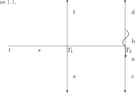
Suppose a FRA for the period [𝑇1, 𝑇2] is entered into at time𝑡with a ﬁxed rate of𝑟𝐾. Suppose we

are now at time𝑠, with 𝑡 < 𝑠 < 𝑇1. How do we value the FRA?

Consider Figure1.1.

f

e

b

a d

c

𝑡 𝑠 𝑇1 𝑇2

? 6

?

6

[image:13.612.133.368.219.378.2]

?

Figure 1.1: Valuing an oﬀ the run FRA

The value of the long position in the FRA is the portfolio given by a and b. a is a notional of

𝑟𝐾(𝑇2−𝑇1), b is the ﬂoating payment on the notional of 1. But I add in c, d, e, and f, and the

value of this is 0, because there is cancellation. All four of these deals have a face value of 1. However, the value of the portfolio given by b, d and e is also 0: it is a position in a ﬂoating rate note. Hence, the value of the FRA is given by the value of a, c and f, which is given by

𝑉(𝑠) = 𝑍(𝑠, 𝑇1)−𝑍(𝑠, 𝑇2)[1 +𝑟𝐾(𝑇2−𝑇1)] (1.15)

One has to be careful to note the period to which a FRA applies. In an𝑛×𝑚 FRA the forward period starts in𝑛 months modiﬁed following from the deal date. The forward period ends𝑚−𝑛

months modified following from that forward date, and NOT𝑚months modified following from the deal date. Here, typically𝑚−𝑛= 3. We will call this strip of dates the FRA schedule. In a swap, the𝑖𝑡ℎpayment is 3𝑖months modified following from the deal date. We will call this strip of dates the swap schedule. Confusion is easy.

Example 1.6.2. On 4-May-07 the JIBAR rate is 9.208%, the 3v6 FRA rate is 9.270%, and the 6v9 FRA rate is 9.200%. What are the 3, 6 and 9 month rates NACC?

Note that

𝐶(4-May-07,6-Aug-07) =

(

1 + 9.208% 94 365

)

= 1.023714

𝐶(4-May-07;6-Aug-07,6-Nov-07) =

(

1 + 9.270% 92 365

)

= 1.023365

𝐶(4-May-07; 5-Nov-07,5-Feb-08) =

(

1 + 9.200% 92 365

)

(14)

Straight away we have𝑟(6-Aug-07) = 9.101%.

Note that we would really like to have 𝐶(4-May-07; 6-Aug-07,5-Nov-07), but we don’t. Also, we would like the sequence to end on 4-Feb-08, but it doesn’t. So already, some modelling is required. We have

𝐶(4-May-07,6-Nov-07) = 1.023714⋅1.023365 = 1.047633 We now want to ﬁnd𝐶(4-May-07,5-Nov-07).

To model this we interpolate between𝐶(4-May-07,6-Aug-07) and𝐶(4-May-07,6-Nov-07). For rea-sons that are discussed elsewhere, the most desirable simple interpolation scheme is to perform linear interpolation on the logarithm of capitalisation factors - so called raw interpolation. SeeHagan and West[2008].

Thus we model that𝐶(4-May-07,5-Nov-07) = 1.047370. Thus𝑟(5-Nov-07) = 9.131%.

Now

𝐶(4-May-07,5-Feb-08) = 1.047370⋅1.023189 = 1.071658 Now interpolate between𝐶(4-May-07,6-Nov-07) and𝐶(4-May-07,5-Feb-08) to get

𝐶(4-May-07,4-Feb-08) = 1.071391 Thus𝑟(4-Feb-08) = 9.119%.

Even within this model, the solution has not been unique. For example, we could have used

𝐶(4-May-07,6-Aug-07) and 𝐶(4-May-07;6-Aug-07,6-Nov-07) unchanged, and interpolated within

𝐶(4-May-07; 5-Nov-07,5-Feb-08) to obtain 𝐶(4-May-07; 6-Nov-07,4-Feb-08). However, this is quite an ad hoc approach. It makes sense to decree that one strictly works from left to right.

1.7 Exercises

1. You have a choice of 2 investments:

(i) R100 000 invested at 12.60% NACS for 1 year

(ii) R100 000 invested at 12.50% NACQ for 1 year.

Which one do you take and why? (Explain Fully)

2. On 17-Jun-08 you sell a 1 Million, 3 month JIBAR instrument. At maturity you receive R1,030,246.58. What was the JIBAR rate?

3. (a) If I have an x% NACA rate, what is the general formula for y, the equivalent NACD rate in i.t.o x?

(b) Now generalise this to convert fromany given rate, 𝑟1 (compounding frequency𝑑1) to

another rate𝑟2(compounding frequency𝑑2).

(15)

4. On 17-Jun-08 you are given that the 3-month JIBAR rate is 12.00% and the 3x6-FRA rate is 12.10%. What is the 6 month JIBAR rate?

5. If the 4 year rate is 9.00% NACM and the 6 year rate is 9.20% NACA, what is the 2 year forward rate (NACA) for 4 years time?

6. Suppose on 22-Jan-08 the 3 month JIBAR rate is 10.20% and the 6 month JIBAR rate is 10.25%. Show that the fair 3x6 FRA rate is 10.0446%.

7. Suppose on 3-Jan-08 a 6x9 FRA was traded at a rate of 12.00%. It is now 3-Apr-08. The NACC yield curve has the following functional form: 𝑟(𝑡, 𝑇) = 11.50% + 0.01(𝑇−𝑡)−0.0001(𝑇−𝑡)2

where time as usual is measured in years. Find the MtM of the receive ﬁxed, pay ﬂoating position in the FRA.

(16)

Chapter 2

The short term rates in the market

The yield curve deﬁnes the relationship between term to maturity and interest rates, for a speciﬁc quality of credit. Typically, a yield curve starts with the overnight point and extends to the 30 year point. In this chapter we look at the overnight and other short term points of the yield curve.

2.1 The repo rate of the SARB

The repurchase (repo) rate of the SARB is the mother of all overnight rates. This rate is set by the South African Reserve Bank (SARB), which is the central bank of South Africa, and it directly aﬀects all other overnight rates that are traded in the market (and it indirectly aﬀects all the rates along the rest of the yield curve).

While the repo rate aﬀects all interest rates in the economy, it is only used for transactions between banks and the SARB. To understand how this works we have to look at the function of the SARB. The SARB conducts the monetary policy of the country. The primary aim of its monetary policy is “to protect the value of the currency in order to obtain balanced and sustainable economic growth in the country”South African Reserve Bank[6 April 2000]. To achieve this, the SARB has two jobs: (1) to achieve price stability and (2) to maintain stable conditions in the ﬁnancial sector. To achieve these goals, the SARB operates in the domestic money market. These money market operations are carried out by the Financial Markets Department at the SARB and involves the control over the supply of funds in the interbank market.

By changing the supply of funds, the SARB can affect short term interest rates (which are determined by the demand and supply of funds), which in turn affects the entire yield curve. This in turn affects the overall level of economic activity in the country and hence the general level of prices.

How does the SARB achieve this? Banks need to hold balances with the SARB. These balances are held for two reasons. Firstly, banks require suﬃcient funds to square oﬀ their positions with each other. The second reason is a statutory requirement which compels banks to hold cash reserve deposits with the SARB.

(17)

balances at the SARB. In this way the SARB acts as the banker to all the banks.

If there was no inﬂow or outﬂow of cash into the banking system and there was a perfect interbank market, the pool of funds would remain the same, banks would never have to borrow money from the SARB and the repo rate would have no teeth. But in reality, there are several transactions that reduce the balances of banks at the SARB. Such transactions increase the liquidity requirement of banks and force them to borrow money from the SARB. Examples of these transactions include an increase in the notes and coins in circulation outside the SARB, an increase in government deposits with the SARB and the selling of gold and other foreign reserves by the SARB to banks.

While these transactions can reduce the balances of banks at the SARB, similar transactions in the opposite direction can also increase their balances. To ensure that banks are always forced to borrow from the SARB so that the repo rate remains eﬀective, the SARB prefers to keep the market “short”. They therefore intervene in the market to create a shortage.

The SARB uses several tools of intervention to create such a shortage. The primary tool goes back to the statutory requirement that we already mentioned. Banks are required by law to hold a percentage (2.5% at present) of their total liabilities (think of it as the public’s deposits with banks) as a cash reserve deposit at the SARB. This permanently drains liquidity from the money market and forces the banks to borrow money from the SARB.

A second tool involves the purchase and sale of SARB debentures to banks. This falls under the broader heading of open market operations. The purchase (sale) of debentures by banks drains (injects) liquidity and forces them to borrow more (less) from the SARB.

Other tools include longer term reverse repos (see Chapter 6) and foreign exchange swaps.

Once the SARB has drained suﬃcient liquidity, the banks have insuﬃcient balances with the SARB and are forced to borrow the shortfall from the SARB.

The SARB is in the process of changing the way in which it conducts its money market operations. A consultative paper appeared in December 2004. Here we briefly outline the current system. The SARB currently uses five methods of refinancing:

1. Refinancing repo auctions. This is the main source of refinancing. These repurchase agreements are a form of securitised lending. (Please note that although this is a form of securitised lending, it differs from the buy-sell back transactions (carries) that are discussed in Chapter7.)

Banks can oﬀer certain ﬁnancial instruments to the SARB and borrow money against these securities. At maturity the banks pay the principal plus interest to the SARB in exchange for their security. The instruments that qualify as security include central government bonds, Treasury bills, Land bank bills and SARB debentures (proposals are under consideration to include government guaranteed bonds). Note that these instruments are held by banks in their normal course of business as liquid assets. The value of the security has to exceed the amount of the loan to insulate the SARB from adverse movements in the market. These “haircuts” are calculated on the market value of the instruments and vary according to their maturity.

The reﬁnancing repo auctions currently take place on Wednesdays and the banks borrow the money from the SARB for a week. The simple interest rate convention is used to calculate the size of the interest payments, on an actual/365 basis.

(18)

liquidity requirement that the SARB estimates and the actual liquidity requirement. Under these conditions the SARB may announce a supplementary auction. The only diﬀerence is that these repos have maturities of one day, and not one week as with the main auctions. The rest of the mechanics is the same: The same instruments qualify as security, the interest calculation convention is simple and the interest rate is equal to the repo rate. It is worth noting that these can be repos or reverse repos, depending if the market is short or long of liquidity.

3. Final-clearing repo auctions. If the difference between the actual and estimated liquidity require-ment is small and if the SARB is not responsible for the estimation error, the banks may have to resort to the final-clearing repo auctions. The mechanics are once again the same, but the interest rate is different in this case. The SARB may impose a penalty (currently 150 bps) on these auctions, where funds are borrowed 150 bps above the repo rate (short liquidity) or invested 150 bps below the repo rate (long liquidity).

4. Marginal lending facility. If banks are not squared oﬀ and fail to make use of the ﬁnal-clearing repos, their accounts are automatically squared at the marginal lending rate. This takes place at a very prohibitive rate, where money is currently borrowed at 500 bps above the repo rate and invested at 0%. This facility however rarely gets used.

5. Access to statutory cash reserve deposits. Recall that banks are required by law to hold a percentage (2.5% at present) of their total liabilities as a cash reserve deposit at the SARB. As long as banks comply with the minimum amount of cash reserves on an average basis during the maintenance period (from the 15th working day of every month to the 14th working day of the following month), they can deposit and withdraw from their cash reserve deposit. The cash reserve deposit does not earn any interest at the SARB.

The SARB is currently proposing a change to the reﬁnancing facilitiesSouth African Reserve Bank

[December 2004]. In short, the SARB wants to use the main refinancing repo auctions, thereafter access to the cash reserve deposits of the banks and lastly the final-clearing repo auctions as the main tools for refinancing. This will essentially create a corridor (floor and ceiling) around the repo rate for interbank rates. The width of the corridor will depend on the penalty associated with the final-clearing repo. It is proposed to narrow this corridor to 50 bps above and below the repo rate. How do changes in the repo rate affect inflation? One of the goals of monetary policy is to maintain price stability. The SARB uses an inflation targeting approach to achieve this. The present target is to keep the year-on-year increase in the CPIX (consumer price index excluding mortgage interest cost for metropolitan and other urban areas) within the range of 3% to 6%.

The SARB uses the repo rate to achieve this inﬂation target. The Monetary Policy Committee (MPC), which is chaired by the Governor of the SARB, meets at least every two months to decide if there should be any changes to the repo rate.

(19)

Finally, you may have noticed that the main reﬁnancing repo auction is a one-week transaction whereas overnight transactions are, well, overnight. This assumes a ﬂat yield curve between one day and one week.

2.2 Call rates

Practitioners use the words call rate and overnight rate as synonyms. There are two types of call transactions, the ﬁrst takes place between banks (interbank call) and the second takes place between banks and their customers. Banks may have diﬀerent call rates depending on the type of customer. The calculations for interbank call and wholesale call are the same.

2.3 Prime rate

[image:19.612.143.434.445.620.2]

Although the prime rate is not strictly speaking an overnight rate, we discuss it here since banks may link some of their overnight transactions to the prime rate. The prime rate is an announced reference rate at which some low risk clients borrow from banks. Distinction is made between the prime mortgage rate which is used for home loans and the prime overdraft rate which is used for credit card transactions, for example. It is quoted as a simple rate. Interest accrues to the account on the last day of every month. The prime rate generally changes when the repo rate changes. Furthermore, a signiﬁcant relationship appears to exist between the prime rate and any of the JIBAR rates.

Figure 2.1: repo, JIBAR and Prime Rates

We can model the prime rate as a function of the one month JIBAR rate, and hence as a function of the yield curve, using a co-integration technique discussed in Alexander [2001], and for this particular case inWest[2008]. Such models have a very high 𝑅2 _{regression coeﬃcient (98% under}

(20)

[image:20.612.144.434.223.398.2]

We see how the model replicates the prime rate in Figure 2.2. One should notice how the cointe-gration smoothes out the jumps to a great extent, as occurs, for example, throughout 2002. This is due to the fact that the market is pricing into the JIBAR rates anticipated jumps to the prime rate before they occur. Only in cases where the quantum of the jump in prime is unexpected in equilibrium - as in August 2004 - does a jump in JIBAR, and consequentially in the replicating function, occur.

Figure 2.2: The replicating function

2.4 Other overnight rates

In addition to interbank and wholesale call transactions, there are also other transactions that have a maturity of one day. These include buy-sell back transactions (carries) and foreign exchange forwards. Carries are discussed in Chapter7.

2.5 Indices of overnight rates

To trade in any market, you need to know what the bid and oﬀer rates are. In many markets there is an exchange that facilitates such price discovery, think of the JSE. When trading the overnight area of the yield curve there is limited transparency.

To establish the true overnight rate is unfortunately not so simple. Firstly, there are several diﬀerent overnight transactions, such as wholesale call, interbank call, carries and forex forwards and there is potentially a diﬀerent rate for each of these. You therefore need to be very clear why you are building the yield curve to ensure that you reference the correct type of overnight rate.

(21)

market is by phone since the screen rates are not always up to date or may only apply to limited volumes. Even though overnight rates don’t change much (if at all) during a day, you can imagine what a rigmarole price discovery can be in this market.

There are two indices of overnight rates available in the market. Neither of them is perfect.

2.5.1 SAONIA rate

To facilitate price discovery in the overnight market the SARB compiles the South African Overnight Interbank Average (SAONIA) rate. As its name indicates, this is an index of interbank transactions only.

The SAONIA rate is the weighted average rate paid on unsecured, interbank, overnight funding. This excludes funding that is raised at the prevailing repo rate. (When the latter is included it constitutes the SAONIA plus rate).

Since the SAONIA rate is based on call rates, the interest calculation is identical to that of call rates.

Although the SAONIA rate was launched with the best intentions, it has not achieved everything that it was designed for. Eﬀorts are currently underway to strengthen the interbank market which should in turn make the SAONIA rate more usefulSouth African Reserve Bank[December 2004].

2.5.2 Safex Overnight rate

During their normal course of business, members of Safex place margin with the exchange to ensure that their contracts are honoured. We will deal with this in Chapter 10. These funds are placed overnight at call rates with F1 and A1 banks.

Safex publishes the Safex Overnight rate which is the average rate that it receives on its deposits with the banks, weighted by the size of the investments placed at each bank. Safex only publishes the average rate and not its composition.

Since the Safex overnight rate is based on call rates, the interest calculation is identical to that of call rates.

It should be noted that Safex tries to earn the highest interest for its clients. In addition, Safex deposits represent a very small portion of the overnight funding in South Africa. The Safex overnight rate may therefore not be a good reﬂection of the weighted average call rates paid on rand deposits by all banks.

(22)

Chapter 3

Swaps

3.1 Introduction

These are identical to the swaps in [Hull,2005, Chapter 7], so refer there for any clarification needed. A plain vanilla swap is a swap of domestic cash flows, which are related to interest rates. We have a fixed payer and a floating payer; the fixed payer receives the floating payments and the floating payer receives the fixed payments.

In South Africa, the arrangements for a swap are as follows: the fixed payments are a fixed interest rate paid on an actual/365 basis on some unit notional, which we will make 1. These interest rates are made in arrears (at the end of fixed periods), and these periods are always three monthly periods. The 𝑖𝑡ℎ payment is on date ModFol(𝑡,3𝑖) where 𝑡 is the initiation date of the product, and the period to which the actual/365 day count applies is the period from ModFol(𝑡,3(𝑖−1)) to ModFol(𝑡,3𝑖). Thus, a swap is not merely a strip of FRAs: not only are payments in arrears and not in advance, the day count schedule is slightly different. The floating payments are on a floating interest rate, paid on the same day count basis, and at the same time, on the same notional. The floating rate will be the 3 month JIBAR rate. As we do not know what the JIBAR rate will be in the future, we do not know what these floating payments will be, except for the next one (because that is already set - remember that the rate is set at the beginning of the 3 month period and the interest is paid at the end of the period). The date where the rate is set is known as the reset date. In other countries, variations are possible. Of course the day count rule could be different. More importantly, it is common for the fixed payments to be made every six months, the floating payments to be made every three months. In these notes, we will in general stick to the situation where the time schedule for the fixed and floating legs are the same.

The notionals are never exchanged, although for some calculation purposes we often imagine that they are, as we will see later. In some more exotic swaps, such as currency swaps, the notional is exchanged at the beginning and at the termination of the product. Of course the fixed and floating payments, occurring on the same day, are net settled. We can, if we like, imagine that notionals ARE exchanged, because they would cancel off net as well. This trick is very useful.

(23)

𝑡0

? 6

𝑡1

?

𝑡2

? ? ? ?

[image:23.612.139.443.112.179.2]

𝑡𝑛

Figure 3.1: Fixed payments (straight lines) and ﬂoating payments (wavy lines)

in the positive direction. We don’t know what the ﬂoating payment is going to be until the ﬁxing date (3 months prior to payment).

3.2 Rationale for entering into swaps

Why would somebody wish to enter into a swap? This is dealt with in great detail in [Hull, 2005, Chapter 7]. The fundamental reason is to transform assets or liabilities from the one type into the other. If a company has assets of the one type and liabilities of the other, they are severely exposed to possible changes in the yield curve. Another reason dealt with there is the Comparative Advantage argument, but this is quite a theoretical concept.

Example 3.2.1. A service provider who charges a monthly premium (for example, DSTV, news-paper delivery, etc.) has undertaken with their clients not to increase the premium for the next year. Thus, their revenues are more or less fixed. However, the payments they make (salaries, interest on loans, purchase of equipment) are floating and/or related to the rate of inflation, which is cointegrated1 with the floating interest rate. Thus, they would like to enter a swap where they pay fixed and receive floating. They ask their merchant bank to take the other side of the swap. This removes the risk of mismatches in their income and expenditure.

Example 3.2.2. A company that leases out cars on a long term basis receives income that is linked to the prime interest rate, again, this is cointegrated with the JIBAR rate. In order to raise capital for a significant purchase, adding to their fleet, they have issued a fixed coupon bond in the bond market. Thus, they would like to enter a swap where they pay floating and receive fixed. They ask their merchant bank to take the other side of the swap. This removes the risk of mismatches in their income and expenditure.

Of course, if the service provider and the car lease company know about each other’s needs, they could arrange the transaction between themselves directly. Instead, they each go to their merchant bank, because

• they don’t know about each other: they leave their ﬁnance arrangements to specialists.

• they don’t wish to take on the credit risk of an unrelated counterparty, rather, a bank, where credit riskiness is supposedly fairly transparent.

1_{A statistical term, for two time series, meaning that they more or less move together over time. It is a diﬀerent}

(24)

• they wish to specify the volume and tenor, the merchant bank will accommodate this; the other counterparty will have the wrong volume and tenor.

• they don’t have the resources, sophistication or administration to price or manage the deal.

Sometimes the above arguments are not too convincing. Thus in some instances major service organisations form their own banks or treasuries - for example, Imperial Bank, Eskom Treasury, SAA Treasury, etc.

3.3 Valuation of a just started swap

How do we value such a swap? Assume that we know the capitalisation function (equivalently, the discount function) for every expiry date𝑇,𝑡 < 𝑇 <∞. The ﬁxed payments are clearly worth

𝑉fix=𝑅

𝑛

∑

𝑖=1

𝛼𝑖𝑍(𝑡, 𝑡𝑖) (3.1)

where𝑅is the agreed ﬁxed rate (known as the swap rate),𝑛is the number of payments outstanding, and𝛼𝑖 is the length of the𝑖𝑡ℎ3 month period on an actual/365 basis. This valuation formula holds whether or not today𝑡 is a reset date.

The valuation of the ﬂoating payments is more tricky. First we value the whole deal, that will give us certain ideas which will enable us to value each ﬂoating payment individually.

Imagine that the notional of 1 is indeed paid at the end. Thus, we have floating interest payments on a notional of 1, paid in arrears every 3 months (as they should be - JIBAR is a yield rate), a final floating interest payment, and repayment of 1 at the end. This deal has a value of 1. Thus, the actual deal (without the payment of notional at the end) has a value of 1 less the present value of that notional, i.e.

𝑉float = 1−𝑍(𝑡, 𝑡𝑛) (3.2)

We can actually make a more complicated argument (to get to the same answer), this alternative argument will have the virtue that we can find the present value of each of the floating payments. We would like to know the value of a single floating in arrears payment. Consider the single payment, which is the payment of interest in arrears of the period [𝑡𝑗−1, 𝑡𝑗] for the interest, on an outstanding loan of 1, which has accrued in that period. How do we value this payment? Consider the following diagram.

The payment we wish to value is the wavy line (its size is not known up front). Again I add in b, c, d, and e, and the value of this is 0, because there is cancelation. All four of these deals have a face value of 1. And as before, a, c and e represent a ﬂoating rate note, also of value 0. Thus

𝑉𝑎 =𝑉𝑎+𝑉𝑏+𝑉𝑐+𝑉𝑑+𝑉𝑒=𝑉𝑑+𝑉𝑏=𝑍(𝑡, 𝑡𝑗−1)−𝑍(𝑡, 𝑡𝑗) (3.3) Thus for a general ﬁxed for ﬂoating swap,

𝑉float =

𝑛

∑

𝑗=1

𝑍(𝑡, 𝑡𝑗−1)−𝑍(𝑡, 𝑡𝑗)

(25)

𝑡

e

a c

b d

𝑡𝑗−1 𝑡𝑗

6

? 6

[image:25.612.130.444.94.261.2]

?

Figure 3.2: A complicated way of getting a single payment!

as a telescoping series.

In the typical situation,𝑡0=𝑡, and so𝑍(𝑡, 𝑡0) = 1. But the above argument is also valid for a swap

which starts at some date𝑡0 in the future. To ‘start’ here means that the ﬁrst observation of the

unknown floating rate is made at that date and the first fixed for floating exchange is made at the observation date that follows that date (for example, 3 months later).

On initiation, a swap is usually struck so that the value of the ﬁxed and ﬂoating payments are equal. Given the𝑍/𝐶 function, it is fairly trivial to solve for the rate𝑅𝑛 that achieves this:

𝑅𝑛=

1−𝑍(𝑡, 𝑡𝑛)

∑𝑛

𝑖=1𝛼𝑖𝑍(𝑡, 𝑡𝑖)

(3.5)

𝑅𝑛 is called the swap rate. Of course, when a bank does such a deal with a corporate client, they will weight the actual𝑅𝑛 traded in their favour.

This view has𝑅𝑛 as a function of the𝑍 function. In fact the functional status is exactly the other way round when we do bootstrapping.

3.4 Valuation of oﬀ the run swaps

Now suppose that 𝑡 is not a reset date. Thus, we reset some time previously, and we are in the ‘middle’ of a 3 month period. To save on introducing more notation, we suppose that the upcoming payment has𝑖index𝑖= 1.

In this case, the formula for the value of the ﬁxed payments is unchanged.

𝑟1_fixhas already been ﬁxed, at the previous reset date.

Again imagine that the notional is indeed paid at the end. When we reach the next reset date, after the ﬂoating payment (which we already know to be 𝑟1

fix𝛼1) is made, the ﬂoating leg will again be

worth 1. Thus, the full deal is currently worth

𝑍(𝑡, 𝑡1)[𝑟1fix𝛼1+ 1]

However, the notional will not be paid on termination, so we need to remove it. Thus

(26)

Alternatively, we can realise that the floating leg is now effectively a fixed payment at𝑡1and floating

payments at𝑡2, 𝑡3, . . . , 𝑡𝑛. Thus

𝑉float = 𝑍(𝑡, 𝑡1)𝑟1fix𝛼1+

𝑛

∑

𝑗=2

𝑍(𝑡, 𝑡𝑖−1)−𝑍(𝑡, 𝑡𝑖)

= 𝑍(𝑡, 𝑡1)𝑟1fix𝛼1+𝑍(𝑡, 𝑡1)−𝑍(𝑡, 𝑡𝑛)

(27)

Chapter 4

BESA Bond Pricing

The issuing of bonds has been the main mechanism for government and high credit worthy insti-tutions borrowing from the public. Government issues (bonds preﬁxed by an r) comprise about 80% of the market. There is about R382b in outstanding debt in the market. This is the primary market: the issuing of bonds. In the secondary market, there are about 2000 trades per day at the Bond Exchange of South Africa (BESA), invoving a nominal of about R42b. The turnover velocity of bonds at BESA is about 28 ie. on average a bond is bought and sold 28 times per year. Therefore we have a very liquid market.

Bonds trade on yield, not on price. Only the South African, Swedish and Australian markets have this feature. This feature is clearly superior, and is possible because the South African bond market opened in 1973 whereas others opened much earlier eg. the UK in the 1600’s. The yield is the IRR as previously, now called the ytm. It is a NACS rate; coupons are semiannual. There is an inverse relationship between yield and price.

Because the market trades on yield but settles on price (the cash price) we need precise rules to take care of the issues that arise. SeeBond Exchange of South Africa[2005].

These speciﬁcations suﬀer from the following defects

• the standard unit is a R100 bond. It would be more natural for the standard unit to be R1 (unitless) or R1m, which is the unit a bond does actually trade in. This amount is called the notional, capital, or bullet. We will price everything as a R1 or unitless bond.

• Some of the derivatives are found in a very complicated manner, and can be simpliﬁed both for esthetic and computational reasons.

Pricing rules need to take care of

• all timing issues,

• coupons are not only in whole multiples of 6 months away,

• that there are books close dates,

(28)

4.1 The Bond Pricing Formula

The pricing mechanism is as follows. Suppose the settlement date is𝑠.

Every bond has two Coupon Dates and two Books Close Dates per annum, notated in the form mmdd. Thus, for example, the CDs of the r153 are 831 and 228, and the BCDs are 731 and 131. Note that the coupon will ﬂow according to the regular following business day rule: this is the day in question if it is a business day, and the next business day if not, but here Saturdays are treated as business days (until they are in their own right public holidays). However, the pricing formula will work as if coupons are paid exactly on the coupon dates.

We will use the following notation:

Abbreviation Notation Meaning Explanation

LCD ℒ Last coupon date The CD before or on 𝑠

NCD 𝒩 Next coupon date The CD after𝑠

BCD ℬ Book’s close date The BCD of the NCD

ℬ was typically one month before 𝒩. However, in 2004, a number of BESA bonds changed their BCD rule, in order to come into line with international conventions. The bonds that changed were essentially government bonds: r and z bonds, Bophuthatswana bonds, Transkei bonds, Umgeni bonds, WS (TransCaledonian) bonds.1 _{The rule is as follows: if}

• the bond is one of these bonds, and

• the LCD is after 31 Dec 2003, and

• the NCD is after 29 Feb 2004

then the NCD is unchanged, while the BCD is 10 calendar days before the NCD. It is important to be able to determine whether or not we are before or after the change, otherwise historical calculations will be invalid. Thus, one does not simply hard-code the new BCD.

It is possible to develop very compact and eﬃcient logic for calculating these dates.

1. Determineℒ,𝒩 such thatℒ ≤𝑠 <𝒩;ℬis that one corresponding to𝒩.2 2. 𝑒=

{

1 if 𝑠 <ℬ

0 if 𝑠≥ ℬ is called the ‘cumex’ ﬂag.

The cumex ﬂag is an indicator of the ownership of the coupon. ℬis the date (up to but NOT including) when whoever the owner was beforeℬis the person who receives the coupon on𝒩. If you sell the bond on or after ℬyou will still receive the coupon. Thus 𝑒indicates whether or not the bond is being sold with the next coupon.

1_{When using excel functionality, is is important to ensure that the input ‘r153’ is that string and not 153 South}

African Rands! Excel will display R 153 (note the space) but the cell is actually populated by the number 153 (an example of what you see is what you typed, but what you get isn’t). This occurs if the currency of the computer has been set to ZAR (of course completely typical). The solution is simple: set the format of the cell where the bond code is to be input to be text: format - cells - number - text.

2_{As an example: for the r153, suppose}_𝑠_{is 27 Feb 2004. Then}_ℒ_{is 31 Aug 2003,}_𝒩 _{is 28 Feb 2004, and}_ℬ_{is 31}

(29)

[ ℒ

𝑒= 1 ℬ )[ 𝑒= 0

𝒩 )

Figure 4.1: The LCD, BCD and NCD

3. Price all cash ﬂows as if we were standing at𝒩.

𝑑= (1 +𝑦₂)−1is the semi-annual discount factor.

𝑛 =[Maturity₁₈₂_.₆₂₅−𝒩] is the number of coupons from the 𝒩 until maturity, not including the one at𝒩.

𝑉𝒩 =

𝑐

2(𝑒+𝑑+𝑑

2₊_{⋅ ⋅ ⋅}₊_𝑑𝑛_{) +}_𝑑𝑛₌ 𝑐 2

(

𝑒+𝑑1−𝑑

𝑛

1−𝑑

)

+𝑑𝑛

where 𝑐is the annual coupon percentage.

4. Calculate the discount factor that takes us from𝒩 back to𝑠.

𝑏=

{ _{𝒩 −}_𝑠

𝒩 −ℒ if 𝒩 ∕= Maturity 𝒩 −𝑠

182.5 if 𝒩 = Maturity

𝑔=

{

𝑑𝑏 _if _{𝒩 ∕= Maturity} 𝑑

𝑑+𝑏(1−𝑑) if 𝒩 = Maturity

are called the broken period and broken period factor respectively.

Note that 𝑑 𝑑+𝑏(1−𝑑) =

(

1 +𝑏𝑦₂)−1

.

The reason we make distinction is in last period before maturity the bond becomes a money market instrument, and 365 days makes the pricing formula consistent with money market day count conventions.

5. The all-in price is

𝔸=𝑔⋅𝑉𝒩 (4.1)

In reality, the market trades𝔸at 𝑡+ 3.3 For example, we trade the r153on the 15-Feb-07. This is

the valuation date. The settlement date is 20-Feb-07. Thus the bond trades ex-coupon ie. 𝑒= 0.

𝑡+ 3 is known as the standard settlement date of𝑡and is denoted𝑠𝑠𝑑(𝑡).

4.2 Rounding

Traders often think in terms of clean price rather than all in prices. Roughly, the clean price is the price without the next coupon having an impact. How is this calculated?

1. The unrounded all-in Price𝔸is calculated as above.

3_{In other words, 3 business days after the actual trade date. Thus one must take care of weekends and public}

(30)

[image:30.612.140.435.124.306.2]

Figure 4.2: There are plenty of anomalies to the clean price formula

2. We calculate how many days𝒟of accrued interest is included in the bond.

𝒟=

{

𝑠− ℒ if 𝑒= 1

𝑠− 𝒩 if 𝑒= 0 (4.2)

Then

Accrued Interest =𝑐 𝒟

365 (4.3)

Of course, there is an anomaly here - compare with the very precise day count methodology seen earlier.

3. The Clean Price is the All in Price minus the Accrued Interest.

4. Round the Clean Price and the Accrued Interest.

5. The Rounded All in Price is the sum of the Rounded Clean Price and the Rounded Accrued Interest.

This is often diﬀerent to just rounding the All in Price! The rounded all in price will be denoted by [_𝔸].

Not only is the day count anomalous, but furthermore the accrual of interest is simple (linear). It would be better if interest accrued by compounding, as typically interest does.

SeeEtheredge and West[1999].

4.3 Risk Measures Associated with Bonds

(31)

Recall that by Taylor series

𝑓(𝑦+ Δ𝑦)−𝑓(𝑦) =𝑓′(𝑦)Δ𝑦+1 2𝑓

′′₍_𝑦_)(Δ_𝑦₎2₊1

6𝑓

′′′₍_𝑦_)(Δ_𝑦₎3₊

⋅ ⋅ ⋅

and so

Δ𝔸= ∂𝔸

∂𝑦Δ𝑦+

1 2

∂2𝔸

∂𝑦2(Δ𝑦) 2₊1

6

∂3𝔸

∂𝑦3(Δ𝑦)

3₊_{⋅ ⋅ ⋅} _(4.4)

We have the following terms

∂_𝔸

∂𝑦 called Delta (4.5)

∂2𝔸

∂𝑦2 called Gamma (4.6)

∂3 𝔸

∂𝑦3 called Speed (4.7)

− ∂𝔸

∂𝑦

𝔸 called Modiﬁed duration, in years (4.8)

−(1 +𝑦 2)

∂𝔸

∂𝑦

𝔸

called Duration, in years (4.9)

∂2𝔸

∂𝑦2

𝔸

called Convexity (4.10)

∂𝔸

∂𝑦 is negative because there is an inverse relationship between yield and price. For a R1 bond, ∂𝔸

∂𝑦 is−3 say. If I have a R1 bond, and𝑦 increases by 1 basis point (1% of 1%), how much money do I make? △𝔸≈ ∂∂𝑦𝔸△𝑦=−3⋅0.0001 =−0.0003 ie. I lose R0.0003.

By ratio and proportion, if I have R1,000,000 of the same bond and yields go up by 1 basis point, I lose R0.0003⋅1,000,000 = R300. This number is called the Rand per point of the bond. Thus the Rand per point is the proﬁt you make when the yield goes down 1 basis point on a bond of R1m. Now let us perform the required calculations:

Derivatives of𝑔with respect to 𝑑, the semi-annual discount factor:

∂𝑔 ∂𝑑 =

{

𝑏𝑑𝑏−1 if 𝒩 ∕=𝑚𝐵 𝑏

[𝑑+𝑏(1−𝑑)]2 if 𝒩 =𝑚𝐵

(4.11)

∂2_𝑔

∂𝑑2 =

{

𝑏(𝑏−1)𝑑𝑏−2 _if _{𝒩 ∕=}_𝑚

𝐵

−2𝑏(1−𝑏)

(4.12)

∂3_𝑔

∂𝑑3 =

{

𝑏(𝑏−1)(𝑏−2)𝑑𝑏−3 _if _{𝒩 ∕=}_𝑚

𝐵

6𝑏(1−𝑏)2

(32)

Derivatives of𝑉𝒩, the total coupon amount, with respect to 𝑑, the semi-annual discount factor:

∂𝑉𝒩

∂𝑑 = 𝑐

2

𝑛𝑑𝑛+1₋₍_𝑛_{+ 1)}_𝑑𝑛_{+ 1} (𝑑−1)2 +𝑛𝑑

𝑛−1 _(4.14)

∂2_𝑉 𝒩

∂𝑑2 =

𝑐

2

𝑛(𝑛−1)𝑑𝑛+1₋₂₍_𝑛2₋₁₎_𝑑𝑛_{+ (}_𝑛_{+ 1)}_𝑛𝑑𝑛−1₋₂

(𝑑−1)3

+𝑛(𝑛−1)𝑑𝑛−2 (4.15)

∂3_𝑉 𝒩

∂𝑑3 =

𝑐

2

[ ₋₃

(𝑑−1)4[𝑛(𝑛−1)𝑑

𝑛+1₋₂₍_𝑛2₋₁₎_𝑑𝑛_{+ (}_𝑛_{+ 1)}_𝑛𝑑𝑛−1₋_2]

+(𝑛+ 1)𝑛(𝑛−1) (𝑑−1)3 [𝑑

𝑛₋₂_𝑑𝑛−1₊_𝑑𝑛−2_]

]

+𝑛(𝑛−1)(𝑛−2)𝑑𝑛−3 (4.16) The formulae derived above are then used to calculate the derivatives of𝔸, the all-in-price.

∂_𝔸 ∂𝑑 =

∂𝑔 ∂𝑑𝑉𝒩+𝑔

∂𝑉𝒩

∂𝑑 (4.17)

∂2 𝔸

∂𝑑2 =

∂2_𝑔

∂𝑑2𝑉𝒩 + 2

∂𝑔 ∂𝑑

∂𝑉𝒩

∂𝑑 +𝑔 ∂2_𝑉

𝒩

∂𝑑2 (4.18)

∂3 𝔸

∂𝑑3 = 3

∂𝑔 ∂𝑑

∂2_𝑉 𝒩

∂𝑑2 + 3

∂2_𝑔

∂𝑑2

∂𝑉𝒩

∂𝑑 + ∂3_𝑔

∂𝑑3𝑉𝒩+𝑔

∂3_𝑉 𝒩

∂𝑑3 (4.19)

Note that:

∂𝑑 ∂𝑦 =

−1 (1 +𝑦/2)2 ⋅

1 2 =−

𝑑2

2 (4.20)

The derivatives of the bond all-in-price with respect to yield, 𝑦, give the bond delta, gamma and speed:

Δ = ∂𝔸

∂𝑦 = − 𝑑2

2

∂_𝔸

∂𝑑 (4.21)

Γ = ∂

2 𝔸

∂𝑦2 =

𝑑3 2 ∂𝔸 ∂𝑑 + 𝑑4 4

∂2𝔸

∂𝑑2 (4.22)

Speed = ∂

3 𝔸

∂𝑦3 = −

3𝑑4

4

∂𝔸

∂𝑑 −

3𝑑5

4

∂2 𝔸

∂𝑑2 −

𝑑6

8

∂3 𝔸

∂𝑑3 (4.23)

4.4 Exercises

1. Relevant Bond data for a selection of SA bonds is provided. Given Inputs:

• Bond Name • Settlement Date • YTM

build a Bond Calculator to:

(a) Bring in (given the above inputs) all the relevant static data for that particular bond -such as maturity, coupon dates etc. (This will be done by means of an excel vlookup table.)

(33)

• The LCD, BCD and NCD as eﬃciently as possible. A good trick is to break every date you consider into a cell containing the year, a cell containing the month, and a cell containing the day. The logic can then revolve around manipulation with these numbers: manipulation with numbers is so much easier than manipulation with dates. To recover the corresponding date, you use the DATE function.

• The Bond Allin Price, both rounded and unrounded. • The Clean Price, both rounded and unrounded.

• The Accrued interest amount, both rounded and unrounded. • the delta and rand per point;

• the duration and modiﬁed duration; • the gamma and convexity.

This must be done entirely in excel. No macros, no vba.

2. Suppose 𝑉 is the value of a set of cash ﬂows (for example, a bond) which has payments

𝑐1, 𝑐2, . . . , 𝑐𝑛 at times𝑡1, 𝑡2, . . . , 𝑡𝑛. Note that 𝑉 =∑_𝑖𝑐𝑖𝑍(0, 𝑡𝑖) :=∑_𝑖𝑉𝑖 where 𝑍(⋅) is for example calculated oﬀ of a yield curve. If the bond has a NACS yield to maturity 𝑦, then we take 𝑍(0, 𝑡𝑖) = (1 +𝑦₂)−2𝑡𝑖_.

Let𝑤𝑖= 𝑉_𝑉𝑖 be the proportion that the𝑖𝑡ℎcomponent makes up of the total value of the bond. We deﬁne (Macauley) duration and modiﬁed duration as

𝐷=∑ 𝑖

𝑡𝑖𝑤𝑖=

∑

𝑖𝑡𝑖𝑉𝑖

∑

𝑖𝑉𝑖

𝐷𝑚=

𝐷

1 +𝑦₂

Note that the units of Macauley duration and modiﬁed duration are years.

(34)

Chapter 5

Bootstrap of a South African yield

curve

There is a need to value all instruments consistently within a single valuation framework. For this we need a risk free yield curve which will be a NACC zero curve (because this is the standard format, for all option pricing formulae).

Thus, a yield curve is a function𝑟=𝑟(𝜏), where a single payment investment for time𝑡 will earn a rate𝑟=𝑟(𝜏). We create the curve using bootstrapping. We do this using raw data and certain rules.

Such curves have been easily observed in the USA and Europe (in the USA via prices of T-bills and T-bonds which have traded out to a 30 year maturity). With the erosion of liquidity of even these instruments the use of swaps is becoming more common.

5.1 The overnight capitalisation factor

How does the call rate work? In many international markets there exists the possibility for a depositor to place cash with a bank, and obtain the capital back with interest the next day. We easily get the overnight capitalisation factor, and hence we could calculate the overnight NACC rate on our yield curve.

There is in fact no true overnight (call) rate in the South African market. In most cases, the interest is calculated every day, but the interest is only paid at the end of every month. (It is however possible to request payment of the interest when funds are withdrawn during the month. But this is a once oﬀ event.)

To create a yield curve, it is however necessary to include a one-day rate (for example, for pricing of short dated equity derivatives). A number of approaches are possible; all of them are decrees rather than fact.

(35)

compounding of interest. Usually, the depositor leaves its money on deposit for the whole month, receiving their capital back at the end and the arithmetic sum (no compounding) of the interest payments.

It is clear that (for a given overnight rate) the actual capitalisation that the depositor is earning improves during the month, as the payment of interest is occurring relatively earlier. However, as pointed out inBond Exchange of South Africa/Actuarial Society of South Africa[2003], there is no evidence that this factor is taken into consideration.

One approach to calculating the overnight capitalisation factor is:

𝐶(0,1𝑑) =(1 + 𝑟 12

)12/365

(5.1)

Of course, this is equivalent to

𝑑=𝑍(0,1𝑑) =(1 + 𝑟 12

)−12/365

(5.2)

Another approach might be

𝐶(0,1𝑑) = 1 +𝑟 1

365 (5.3)

that is, the overnight rate is modelled as a true overnight rate.

Of course these approaches are plausible art, not science - there is no arbitrage reason why this is the overnight compounding factor. There are other solutions to this problem. Some institutions, for example, calculate the one month rate, and then simply extrapolate horizontally from there back to the 1 day term node. A solution is required, but there is no point in claiming that any given solution is ‘correct’: the overnight compounding factor does not actually exist.

5.2 Bootstrap the money market part of the curve

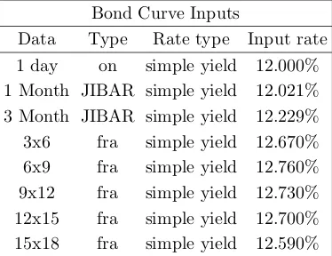
We will consider one bootstrap of a NACC yield curve via an example. Suppose on 17-Jun-08, we have the inputs in Table5.1.

Bond Curve Inputs

[image:35.612.194.381.509.653.2]

Data Type Rate type Input rate 1 day on simple yield 12.000% 1 Month JIBAR simple yield 12.021% 3 Month JIBAR simple yield 12.229% 3x6 fra simple yield 12.670% 6x9 fra simple yield 12.760% 9x12 fra simple yield 12.730% 12x15 fra simple yield 12.700% 15x18 fra simple yield 12.590%

Table 5.1: Money market curve data for 17-Jun-08

(36)

• We will use (5.3) to calculate the overnight rate. 𝐶(0,1𝑑) = 1 + 12.000%

365 = 1.0003288, so

𝑟1𝑑= 365 ln𝐶(0,1𝑑) = 11.9980%. • 𝐶(0,30𝑑) =(

1 + 12.021%30 365

)

= 1.0098803, so𝑟30𝑑= 365₃₀ ln𝐶(0,30𝑑) = 11.9620% • 𝐶(0,92𝑑) =(1 + 12.229%₃₆₅92)= 1.0308238, so𝑟92𝑑= 365₉₂ ln𝐶(0,92𝑑) = 12.0443%

From the above listed observation dates, the fra periods are of length 91, 90, 92, 92, 91 days. We now use (1.12) over and over. Thus

• 𝐶(0,183𝑑) =𝐶(0,92𝑑)⋅[

1 + 12.670%91 365

]

and so𝑟183𝑑= 12.2580% • 𝐶(0,273𝑑) =𝐶(0,183𝑑)⋅[

1 + 12.760%₃₆₅90]and so𝑟273𝑑= 12.3587% • 𝐶(0,365𝑑) =𝐶(0,273𝑑)⋅[

1 + 12.730%₃₆₅92]

and so𝑟365𝑑= 12.4019% • 𝐶(0,457𝑑) =𝐶(0,365𝑑)⋅[

1 + 12.700%₃₆₅92]and so𝑟457𝑑= 12.4218% • 𝐶(0,548𝑑) =𝐶(0,457𝑑)⋅[

1 + 12.590%₃₆₅91]

and so𝑟548𝑑= 12.4176%

5.3 Bootstrap using default-free bonds

In South Africa the traditional approach has been to use JIBAR’s in the short part of the curve, FRA’s in the medium part of the curve and r bonds in the long part of the curve. What is the major diﬀerence between JIBAR’s and Bonds in terms of credit worthiness? In the JIBAR market, if you lend money you may not get it back, but in the bond market you will get it back. Thus diﬀerent levels of credit worthiness are used to construct the curve, although this is forced by the lack of liquid and perfect credits in the short and medium term.

Thus we are looking at a curve which is not default free (and does not ﬁt in with typical theoretical assumptions in options pricing) because there are not government bonds on the left (short) side of the curve. This will not occur in the US - you can construct an entire yield curve just using treasury bills. In SA there are no liquid and short-dated government bonds.

Suppose we also have the input data in Table5.2. Now for the hard step. We only extend the curve

Bond Curve Inputs Data Type Rate type Input rate

[image:36.612.209.367.560.676.2]

r153 Bond ytm 11.590% r201 Bond ytm 10.530% r157 Bond ytm 10.460% r203 Bond ytm 10.450% r204 Bond ytm 10.420% r186 Bond ytm 10.270%

Table 5.2: Bond curve data for 17-Jun-08

(37)

[_𝔸] = 1.0659167 for settlement 20-Jun-08. We will consider two diﬀerent ways of realising this value: [𝔸] exp [−𝑟𝛼𝛼] =

𝑁

∑

𝑖=0

𝑝𝑖exp [−𝑟𝜏𝑖𝜏𝑖] (5.4)

where

𝛼 = 3 business day term, measured in years

𝑝0 = 𝑒

𝑐

2

𝑝1, 𝑝2, . . . , 𝑝𝑁−1 =

𝑐

2

𝑝𝑁 = 1 +

𝑐

2

1

𝑁 = The𝑁 in the bond pricing formula

𝜏𝑖 = term in years until the coupon ﬂow𝑖2

In this example, 𝛼= 3𝑑. Note that this is the critical equation of value: whether we realise the value in the bond market, or we strip the cash ﬂows one at a time, we must (in principle) get the same value.

We will use linear interpolation to ﬁnd the rate at any point which is between known rates3_{. In}

other words, we assume that such rates are known.

Using this interpolation, the 3d rate is 11.9955%. Thus, the left hand side of (5.4) for the r153 is 1.06486629. The cash ﬂows on the right hand side are as in Table5.3.

date cash ﬂow rate pv

[image:37.612.126.464.135.315.2]

01-Sep-08 0.0650000 12.0231% 0.063393 28-Feb-09 0.0650000 12.3396% 0.059611 31-Aug-09 0.0650000 12.4181% 0.055963 17-Dec-09 0.0000000 12.4176% 0.000000 01-Mar-10 0.0650000 ?? ?? 31-Aug-10 1.0650000 ?? ??

Table 5.3: Cash ﬂows for r153, iteration 0

The one equation has two unknowns. What we now do is impose a model - we make𝑟𝑁 the subject of the equation. Hence

𝑟𝜏𝑁 =−

1

𝜏𝑁

[

ln

(

𝔸exp [−𝑟𝛼𝛼]− 𝑁−1

∑

𝑖=0

𝑝𝑖exp [−𝑟𝜏𝑖𝜏𝑖]

)

−ln𝑝𝑁

]

(5.5)

2_{In the case that} _𝑁 _{= 0 we have}_𝑝

𝑁 = 1 +𝑒𝑐2 and the equation that will follow solves immediately, without

iteration.

2_{Note that this is found using the regular following date of the the designated coupon date.} 3_If_{𝑎 < 𝑥 < 𝑏}_{, and we know}_𝑓₍_𝑎_),_𝑓₍_𝑏_{), then}_𝑓₍_𝑥_{) =} 𝑥−𝑎

𝑏−𝑎𝑓(𝑏) + 𝑏−𝑥

𝑏−𝑎𝑓(𝑎). In real applications of this approach, a

South African Financial Markets