RESEARCH
Continuities and changes in spatial
patterns of under-five mortality at the district
level in India (1991–2011)
Akansha Singh
1*and Bruno Masquelier
1,2Abstract
Background: India has the largest number of under-five deaths globally, and large variations in under-five mortality
persist between states and districts. Relationships between under-five mortality and numerous socioeconomic, devel-opment and environmental health factors have been explored at the national and state levels, but the possible spatial heterogeneity in these relationships has seldom been investigated at the district level. This study seeks to unravel local variation in key determinants of under-five mortality based on the 1991 and 2011 censuses.
Methods: Using geocoded district-level data from the last two census rounds (1991 and 2011) and ordinary least
squares and geographically weighted regressions, we identify district-specific relationships between under-five mor-tality rate and a series of determinants for two periods separated by 20 years (1986–1987 and 2006–2007). To identify spatial groupings of coefficients, we perform a cluster analysis based on t-values of the geographically weighted regression.
Results: The geographically weighted regression analysis shows that relationships between the under-five
mortal-ity rate and factors for socioeconomic, development, and environmental health factors vary spatially in terms of direction, strength, and extent when considering: female literacy and labor force participation; share of scheduled castes and scheduled tribes; access to electricity; safe water and sanitation; road infrastructure; and medical facili-ties. This spatial heterogeneity is accompanied by significant changes over time in the roles that these factors play in under-five mortality. Important local determinants of under-five mortality in 2011 were female literacy, female labor force participation, access to sanitation facilities and electricity; while the key local determinants in 1991 were road infrastructure, safe water, and medical facilities. We identify six different clusters based on geographically weighted regression coefficients that broadly encompass the same districts in both periods; but these clusters do not follow the regional boundaries suggested by the previous studies. In particular, the high mortality states of India that are often typically classified as high focus states were classified into three different clusters based on the relationship of the fac-tors associated with under-five mortality.
Conclusion: This study demonstrates the utility of combining geographically weighted regression and cluster
analy-ses as a methodological approach to study local-level variation in public health indicators, and it could be applied in any country using aggregate-level information from census or survey data. Identifying local predictors of under-five mortality is important for designing interventions in specific districts. Additional reduction in under-five mortality will only be possible with intervention programs designed at the local level, which take into consideration local level determinants of under-five mortality.
Keywords: Under-five mortality, India, Geographically weighted regression, District
© The Author(s) 2018. This article is distributed under the terms of the Creative Commons Attribution 4.0 International License (http://creat iveco mmons .org/licen ses/by/4.0/), which permits unrestricted use, distribution, and reproduction in any medium, provided you give appropriate credit to the original author(s) and the source, provide a link to the Creative Commons license, and indicate if changes were made. The Creative Commons Public Domain Dedication waiver (http://creat iveco mmons .org/ publi cdoma in/zero/1.0/) applies to the data made available in this article, unless otherwise stated.
Open Access
*Correspondence: [email protected]
1 Centre de recherche en démographie, Université Catholique de Louvain, Louvain-la-Neuve, Belgium
Introduction
Reducing the under-five mortality rate (U5MR) by two-thirds (between 1990 and 2015) was a key Millennium Development Goal, and tracking progress in this goal has spurred a flurry of methodological developments in gen-erating robust estimates of U5MR at the national scale [1–3]. The focus on levels and trends in U5MR through national averages may have somewhat obfuscated differ-ential progress within countries. The Sustainable Devel-opment Goals (SDG) agenda marks a shift in the fight against child mortality, since increased attention is now devoted to closing equity gaps while reducing the overall level of mortality. The SDG’s U5MR target for 2030 is to end preventable deaths of newborns and children under five years of age. All countries should aim to reduce neo-natal mortality to at least as low as 12 deaths per 1000 live births, and U5MR should be at least as low as 25 deaths per 1000 live births [4]. With this new SDG agenda, it is crucial to develop subnational estimates to ensure that no one is left behind, especially in large and decentralized countries such as India.
With a population of 1.3 billion and U5MR still esti-mated at 43 deaths per 1000 live births in 2016, India has the highest number of child deaths in the world. In 2016, an estimated one million children died in India [5], corresponding to about one-fifth of the global number of under-five deaths. The country failed to achieve the MDG 4 target, despite reducing U5MR by 64% between 1990 and 2015. There are also large variations in U5MR between states [6]. According to the Sample Registra-tion System (SRS) data for the year 2015, the U5MR of Assam in Northeast India was 62 deaths per 1000 live births, which is more than four times higher than that of Kerala in South India, where the U5MR was estimated at 13 per 1000 [7]. Numerous studies have highlighted higher mortality rates in the northern states [8–13] com-pared with states in the southern and western parts of the country. A north–south divide contrasts with inequali-ties in adult mortality, where the largest differences are observed between eastern India and western India [9]. Some studies have also demonstrated that child deaths are highly clustered and that improvements in U5MR have been uneven, with certain hotspots still bearing the brunt of under-five deaths, especially Assam, Madhya Pradesh, Rajasthan, Uttar Pradesh, and Orissa [10, 11]. In this context, achieving the SDG target will require iden-tifying areas that are falling behind and targeting them with specific interventions that will ideally reach beyond the state level. The lowest level of disaggregation in India is the district, which constitutes the basic administra-tive unit. Yet, relaadministra-tively few studies have examined the levels and determinants of U5MR at this level in India. Numerous studies have analyzed cause-specific mortality
changes [12], explored U5MR risk factors at the national or state level [13], or they have classified India into broad geographic regions [8]. Studies that disaggregate their estimates at the district level have focused on develop-ing accurate mortality estimates [14] or investigating sex differentials [15]. However, efforts to identify determi-nants of U5MR at the district level are often restricted to selected states only [10] or to a single census. The work of Bhattacharya [16]—which refers to the period before 2000—and that of Bhattacharya and Chikwama [17]—which refers to the period until 2001—are two noticeable exceptions. These last two studies suggest that variables related to modernization and economic devel-opment (such as access to medical facilities and access to urban areas through paved roads) together accounted for more than 40% of the decline in U5MR during the 1981–1991 period. By contrast, variables related to the agency of women—such as literacy and their participa-tion in the labor market—accounted for only 6% of this decline. These previous studies also indicated that while mortality declined overall, inequalities in child survival increased between 1981 and 2001 [16]. While better access to medical facilities and safe drinking water con-tributed to reducing inequalities, other dimensions of structural change—such as infrastructure development, female literacy, and socio-cultural variables—showed dif-ferential progress and consequently contributed towards increased inequality in U5MR across districts [17]. How-ever, these analyses capture only the overall effects of specific determinants on U5MR. In this paper, we build on these works but additionally investigate the spatial heterogeneity in the relationships between district-level U5MR and a set of significant socioeconomic, develop-ment, and environmental health factors in India, all of which we have based on census data from 1991 and 2011. We focus less on differences between regions and more on differences within regions.
We aim to test whether the associations between U5MR and major determinants vary locally. If this is the case, a single global model may not readily summarize these relationships. For example, female literacy could shape inequalities in U5MR in some specific areas where there are still important gaps in education, but it could play only a minor role when a vast majority of women are literate. We assess spatial heterogeneity in U5MR and the relationships of its associated factors using geographi-cally weighted regression (GWR).
the district level and to capture changes over time in the magnitude and direction of relationships between key determinants and U5MR at the local level. Previous stud-ies using global regression models [16, 17] indicate that the significant factors related to U5MR variation are not the same over these years. We further test U5MR and its predictor’s relationship for regionality by applying cluster analysis to the GWR results. Clustering districts based on the local regression coefficients from GWR analysis iden-tifies regions with similar relationships. Several previous analyses have found geographic variability in regression relationships [18–20], but these analyses are based on predefined regions, and it is possible that these defini-tions influence the chances of finding regional variability. Regional boundaries defined using cluster analysis are data-driven boundaries rather than anything that is pre-defined geographically or based on any single indicator.
Methods Data
Censuses are conducted in India approximately every ten years, with the last three censuses having been con-ducted in 1991, 2001 and 2011. For this analysis, we used district-level data from two rounds of census data (1991 and 2011) provided by the Registrar General of India to estimate U5MR and build a set of explanatory variables.
Outcome variable
Our outcome measure of U5MR is the probability of a newborn dying before reaching age 5 (5q0) if he or she
was exposed to the mortality rates of the period under consideration. All women of childbearing age reported on their total number of children ever born and children surviving in the 1991 and 2011 censuses. This informa-tion was the basis for applying a standard indirect demo-graphic method to estimate mortality, referred to as the Brass method [21]. Using model-based coefficients to account for variations in the age pattern of fertility and
mortality, this method converts the proportion of dead children born to women in each five-year age group into estimates of the probability of dying by exact ages of childhood, and it calculates the number of years before the survey date to which the estimates refer. The indi-rect method, described in detail elsewhere [22], provides one estimate of U5MR for each age group of women. Reports from the youngest women aged 15–19 typically provide mortality rates referring to approximately one or 2 years before data collection and reports from the old-est women refer to a more distant past, sometimes more than 15 years before data collection. For this analysis, we retained the average of estimates derived from two age groups of women (25–29 and 30–34 years old) to get one final estimate per district for each census. We dis-carded reports from younger women aged 15–24 because first-born children and children born to young moth-ers are disproportionately represented in these reports, thus introducing upward biases in mortality rates [22]. We also discarded reports from women older than 35 in order to limit biases due to more frequent omissions of deceased children among older women and due to errors in recalling events that occurred in the more dis-tant past. The reference dates for 5q0 estimates for the
2011 and 1991 censuses are, respectively, 2006–2007 and 1986–1987.
Explanatory variables
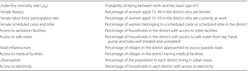
The set of explanatory variables considered in this study is also measured at the district level and constructed from tabulated census data (Table 1). Women’s agency, a key determinant of U5MR, is captured through female lit-eracy among adults aged 15–49 years and through female labor force participation in the age group of 15–59 years. Social variations are reflected in the percentage of females belonging to scheduled castes and scheduled tribes. Scheduled tribes and castes are officially desig-nated groups of disadvantaged people, comprising 8.6%
Table 1 Description of variables used in this study
Under-five mortality rate (5q0) Probability of dying between birth and the exact age of 5
Female literacy Percentage of women aged 15–49 in the district who are literate
Female labor force participation rate Percentage of women aged 15–59 in the district who are currently at work
Female scheduled caste and tribe Percentage of women belonging to a scheduled caste or scheduled tribe in the district Access to sanitation facilities Percentage of households in the district with access to toilet facilities
Access to safe water Percentage of households in the district with access to safe water from tap, hand
pump and tube well (treated and untreated)
Road infrastructure Percentage of villages in the district approached by pucca (paved) roads
Access to medical facilities Percentage of villages in the district having medical facilities
Urbanization Percentage of the population in each district living in urban areas
(when considering tribes) and 16.6% (when consider-ing castes) in the 2011 census. The level of the district’s economic development is captured through the percent-age of villpercent-ages with access to pucca roads (paved roads) and the urbanization level of the district. The relatively healthy character of the environment is reflected in the percentage of villages with access to medical facilities and the percentage of households with access to sanitation facilities and safe water.
Analysis
Some district boundaries have changed between 1991 and 2011. For this study, however, the districts in 1991 were considered as the reference, and districts that had been separated in recent years were merged into the original district. In total, we retained 449 districts. We excluded districts from Jammu and Kashmir, Lakshadweep, and Andaman and Nicobar Islands for the following reasons. One, the census was not conducted in Jammu and Kash-mir in 1991. Two, Lakshadweep, Andaman, and Nicobar are islands and it is therefore difficult to define their spatial neighbors and calculate the bandwidth in GWR.
To capture the pattern and magnitude of spatial ters, we first explored the significant local spatial clus-ters/outliers of U5MR rates using local indicators of spatial association (LISA) statistics [23]. Areas identi-fied as “high–high” refer to districts with above-average U5MR and which also share boundaries with neighbor-ing districts that have above-average U5MR. “High-low” areas point to districts with above-average U5MR and which are surrounded by districts with below-average values. The “high–high” areas are also often referred to as “hot spots”, whereas the “low–low” are referred to as “cold spots”. Spatial dependence in the district-level esti-mates of each indicator was assessed using Moran’s I Index (Global) value. In general, a Moran’s Index value near +1 indicates clustering, while an index value near − 1 indicates dispersion.
Ordinary least squares (OLS) models were used to obtain coefficient estimates at the global level. The OLS models also helped identify the covariates by means of a stepwise approach before moving on to the GWR. The stepwise regression approach selected variables in the OLS model for the 2011 census and these same variables were retained for the 1991 census. Further multicollin-earity tests were performed on the final set of variables. The multicollinearity was assessed through variance inflation factor (VIF) values, and VIFs greater than 10 indicated multicollinearity [24]. This final list of selected variables was retained for both the OLS and GWR analy-ses. To explore the varying relationships between U5MR and socioeconomic predictors, we used GWR models. The bandwidth size was determined by minimizing the
Akaike Information Criterion (AIC). Model compari-sons between the OLS and GWR models were conducted using the AIC with a correction for finite sample sizes (AICc). One of the advantages of GWR modeling is that researchers can map the local coefficients as well as R2 in
order to better identify spatial heterogeneities [25]. Following previous studies [26], the basic equation of the GWR model is expressed as:
where yi refers to the U5MR in the district i; (ui, vi) denotes the coordinates of the centroid of district i; β0i is the local
intercept for the district i; and βni is the local coefficient
for predictor n for district i. This GWR model was run separately for each census (1991, 2011). In GWR models, the regression coefficients are estimated for each district independently by applying location-specific weighting schemes; therefore, there are as many “local” regression models as there are observations [27]. In matrix form, the vector of local coefficients is estimated as:
where X is the matrix of independent variables, and Y
is the vector of dependent variables. The estimator in Eq. (2) is a weighted least squares estimator where the weights vary according to the location point of i. There are a variety of weighting schemes available to choose for researchers [26]. We chose the Gaussian weights and their bi-square variations, which are the most com-monly used options. Thus in Eq. (2), Wi is an n × n diagonal matrix with the j-th diagonal element equal to
1−(dij/b)2 2
if dij < b and zero otherwise. dij refers to the Euclidean distance between location i, where the parameters are estimated, and a specific point in space
j at which data is observed [26]. The parameter b is the bandwidth size (i.e. the distance between each observa-tion and its neighboring locaobserva-tions specified by the spatial weights). Further, a spatial non-stationarity test was con-ducted to test the significance of spatial variability in the local parameter estimates. This was performed using a test developed by Leung and colleagues [28].
Finally, to examine whether there were spatial group-ings of coefficients from the GWR and to facilitate the interpretation of the GWR results, we applied cluster analysis to the t-values (that is, the local regression parameters divided by the standard errors of the esti-mates), which were obtained from the GWR model. We use local t-coefficients instead of the beta coef-ficients because the former denote both the direction
(1) yi =β0i(ui,vi)+
k
n=1
βni(ui,vi)xni+εi
(2) βi=X′WiX−1
and effect size of the relationships [29, 30]. K-means clustering was used to get the final number of clusters to be retained. The optimal number of clusters for the K-means method is chosen based on the Elbow method described elsewhere [31]. It is worth noting that these clusters form areas that are not defined by state boundaries and reflect specific patterns of variations in U5MR. Nor do they coincide exactly with regions high-lighted in previous studies on India. Simple OLS regres-sion was then performed in each cluster to study the relationships that socioeconomic and environmental factors have with U5MR in these specific clusters. All analyses were performed with the R statistical software.
Results
U5MR has declined almost everywhere over the past 20 years, from the period 1986–1987 to 2006–2007, but there are large variations in the pace of decline (Fig. 1).
According to the 1991 census, most 1986–1987 U5MR estimates for the districts in the south of the country varied between 50 and 100 under-5 deaths per 1000 live births, and a few districts had less than 50 under-5 deaths per 1000 live births in the south-west of the country (in Maharashtra, near Mumbai). By comparison, according to estimates at the national level that were developed by UN IGME, the U5MR was estimated at 141 per 1000 in 1986 [5]. U5MR was higher than 100 per 1000 live births in most districts in the northern region, especially in states such as Madhya Pradesh and Uttar Pradesh. There were only modest changes in the geography of U5MR from 1986–1987 to 2006–2007, with a clear cluster of high U5MR districts remaining in the center of the coun-try and low U5MR pockets persisting in the south. In estimates derived from the 2011 census, 22 districts had a U5MR below 50 per 1000 while 333 districts managed to contain their U5MR to between 50 and 100 under-5
deaths per 1000 live births. By comparison, the UN IGME estimate for 2006 was 71 at the national level [5].
The LISA cluster maps presented alongside the map of overall U5MR display four types of geographical cluster-ing for U5MR. These maps indicate persistent geographic clustering of high U5MR in Central India and parts of the east. On the other hand, the maps also show a few cold spots with substantially lower U5MR in South India and in a few districts of Northeast India. The number of districts falling into high–high clusters decreased signifi-cantly from 1991 to 2011. Quite surprisingly, there were no high-low or low–high clusters in 1991, and only one high-low cluster in 2011. Table 2 shows values of Moran’s I statistic, which is a measure of the spatial autocorrela-tion among the neighboring values [23]. Moran’s I sta-tistics for all the variables are relatively high, suggesting
strong spatial patterns for both dependent and independ-ent variables.
Coefficients from the standard OLS model show the expected relationships between district-level U5MR and socioeconomic, development, and environmental health factors (Table 3). They are also broadly consist-ent over time. The global model for 1991 explains 46% of the variation in U5MR, and the model for 2011 explains 52% of the variation. According to estimates from the two censuses, female literacy and labor force participa-tion in a district have significant negative relaparticipa-tionships with U5MR. As the proportion of women belonging to scheduled tribes and castes increases in a district, U5MR also increases significantly. However, the set of indica-tors significantly associated with U5MR is not the same across each census. For example, access to safe water at the household level and the percentage of villages with access to paved roads were significantly associated with U5MR in 1991; whereas in the 2011 census, it was house-holds having access to sanitation facilities and electricity and villages having access to medical facilities that were significantly associated with U5MR.
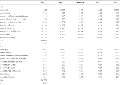
Table 4 provides the estimated coefficients of the GWR model. These coefficients demonstrate how the identi-fied relationships vary from one district to another and to what extent these local relationships remain hidden in the global model presented in the OLS models above. The non-stationarity test results suggest that all the covari-ates are spatially nonstationary and therefore should be treated as local covariates. This observation holds in both census years. In terms of overall goodness-of-fit when comparing to the OLS model, the Quasi-Global R2
is higher than 0.80 for both the GWR models. The AICc
Table 2 Moran’s I test statistics for the different variables under study
*p < 0.05; **p < 0.01; ***p < 0.001
Censuses 1991 2011
Under-five mortality rate 0.64*** 0.60***
Female literacy 0.68*** 0.68***
Female labor force participation rate 0.72*** 0.68***
Female scheduled caste and tribe 0.55*** 0.55***
Access to sanitation facilities 0.38*** 0.70***
Access to safe water 0.60*** 0.63***
Road infrastructure 0.70*** 0.64***
Access to medical Facilities 0.64*** 0.60***
Urbanization 0.13*** 0.33***
Access to electricity 0.64*** 0.77***
Table 3 OLS regression estimates for under-five mortality rate at the district level, in the 1991 and 2011 censuses
vif is variance inflation factor, which quantifies the severity of multicollinearity in an ordinary least squares regression analysis *p < 0.05; **p < 0.01; ***p < 0.001
1991 2011
Estimate Std. error t-value p value vif Estimate Std. error t-value p value vif
(Intercept) 172.54 6.56 26.28 0.00*** 138.78 7.35 18.88 0.00***
Female literacy − 1.08 0.11 − 9.80 0.00*** 2.09 − 0.69 0.10 − 6.99 0.00*** 2.79
Female labor force participation rate − 0.34 0.09 − 3.67 0.00*** 1.67 − 0.21 0.08 − 2.75 0.01** 1.93
Female scheduled caste and tribe 0.16 0.08 2.11 0.04* 1.54 0.27 0.04 6.06 0.00*** 1.69
Access to sanitation facilities 0.07 0.08 0.80 0.43 1.56 − 0.13 0.05 − 2.61 0.01** 2.89
Access to safe water − 0.18 0.07 − 2.54 0.01* 1.34 0.05 0.04 1.17 0.24 1.34
Road infrastructure − 0.33 0.07 − 4.57 0.00*** 2.09 − 0.04 0.03 − 1.32 0.19 1.56
Access to medical facilities − 0.03 0.05 − 0.65 0.52 1.57 − 0.09 0.04 − 2.49 0.01* 1.54
Urbanization − 0.21 0.10 − 2.15 0.03* 1.53 0.18 0.05 3.45 0.00*** 1.93
Access to electricity 0.03 0.08 0.44 0.66 2.18 − 0.18 0.04 − 3.89 0.00*** 3.10
R2 0.46 0.52
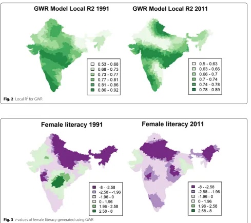
of the GWR model is smaller than the OLS model for both census years, suggesting that the former has a bet-ter fit than the latbet-ter. Local R2 maps (Fig. 2) indicate that
the GWR model fits well in most places in India, with R2 being above 0.50 for all the local models. This value
is higher than the R2 value of the OLS model. The local
R2 values for districts from Maharashtra, Karnataka, and
Andhra Pradesh are higher than 0.80 for both censuses, suggesting that the current set of indicators capture more than 80% of the variation in U5MR in the districts from these regions (Fig. 2).
More importantly, our results demonstrate that rela-tionships between the local variables and U5MR in India vary substantially. This is illustrated in Fig. 3 for female literacy and in “Appendix 1” for all the other covariates, with the t-values of the GWR models included. The green tones represent positive relationships and the purple tones represent negative relationships. Each covariate shows specific spatial variations that cannot be readily sum-marized in terms of a simple pattern (such as the often-mentioned north–south divide in U5MR). For example,
when considering the relationship between U5MR and female literacy, the t-values for 1991 are highly significant and negatively associated with U5MR in the northeast, northern, and central parts of India. However, this asso-ciation was positive and significant for the year 1991 in a series of districts located in the south and in Rajasthan. It is unclear why higher literacy rates could be associated with higher mortality rates in these areas. In 2011, no dis-trict showed a significant positive relationship, and the negative association was significant in half of the districts. Similarly, access to sanitation facilities and access to other facilities can be significantly and positively associated in one region and negatively associated in another. Overall, our GWR analysis clearly suggests that the association of each predictor with U5MR varies significantly over space and time. Distinct regions characterized by positive or negative associations can be discerned with coherent evo-lution over time between the 1991 and 2011 censuses.
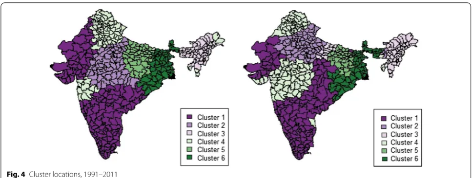
For both censuses, an examination of the percent-age of variance explained as a function of the number of clusters called for dividing India into six principal
Table 4 GWR coefficients for under-five mortality rate at the district level, in the 1991 and 2011 censuses
Non-stationarity test is significant at p < 0.001 for all variables in the GWR model
Min Q1 Median Q3 Max
1991
(Intercept) − 40.09 110.70 152.20 190.30 280.70
Female literacy − 3.18 − 1.27 − 0.60 − 0.08 0.96
Female labor force participation rate − 1.19 − 0.45 − 0.12 0.29 1.31
Female scheduled caste and tribe − 1.04 0.05 0.26 0.49 1.26
Access to sanitation facilities − 2.18 − 0.32 0.08 0.38 1.07
Access to safe water − 1.00 − 0.32 − 0.05 0.20 0.81
Road infrastructure − 1.25 − 0.43 − 0.25 0.13 1.42
Access to medical facilities − 1.35 − 0.33 − 0.14 0.00 0.43
Urbanization − 1.16 − 0.37 − 0.09 0.03 0.63
Access to electricity − 1.13 − 0.50 − 0.26 − 0.03 1.40
AICc 4046.67
R2 0.84
2011
(Intercept) 34.97 116.70 148.90 161.30 197.40
Female literacy − 1.24 − 0.77 − 0.56 − 0.34 0.42
Female labor force participation rate − 1.02 − 0.32 − 0.16 0.19 1.37
Female scheduled caste and tribe − 0.63 0.00 0.12 0.28 0.94
Access to sanitation facilities − 0.86 − 0.33 − 0.13 − 0.01 0.27
Access to safe water − 0.41 − 0.09 0.06 0.23 0.68
Road infrastructure − 0.60 − 0.09 0.01 0.08 0.30
Access to medical facilities − 0.43 − 0.16 − 0.06 0.03 0.54
Urbanization − 0.32 0.01 0.12 0.24 0.73
Access to electricity − 1.51 − 0.40 − 0.28 − 0.10 0.64
AICc 3617.46
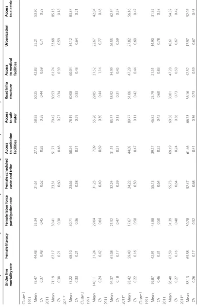
clusters (Fig. 4). It should also be kept in mind that the cluster analysis was performed using t-value estimates of GWR for each census independently (that is, there is no exchange of information between the 1991 and 2011 censuses). In both censuses, 70% of the 449 dis-tricts were part of the same cluster, so these clusters are broadly comparable, even though the shapes and areas covered by each cluster have changed slightly. For example, Cluster 1 is located partly in the south of the country but also with some districts located in the western regions, and it has expanded from 1991 to 2011. For this reason, instead of working with two different sets of clusters, we retained the clusters obtained in 1991 and performed the cluster-specific OLS regressions successively on the 1991 and 2011
data. “Appendix 2” shows descriptive statistics of all the dependent and independent variables considered in this study for each cluster in 1991 and 2011. Compari-son of the descriptive statistics for the year 2011 as per the cluster boundaries for 1991 and 2011 suggests that our conclusions do not substantially change even if we retain the same set of clusters for each census year.
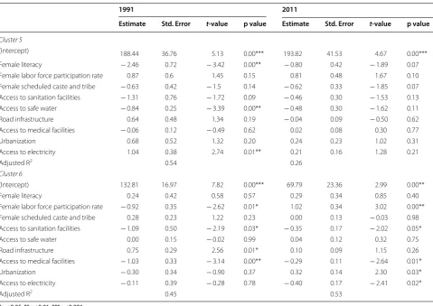
To characterize the clusters, we again performed an OLS regression at the district level for each cluster. Table 5 presents the OLS regression results for each clus-ter in the year 1991 and 2011. “Appendix 2” provides the basic statistics of all independent variables in each clus-ter. Within the same cluster—the factors significant in both years are not precisely the same. We highlight some peculiarities of each cluster below.
Fig. 2 Local R2 for GWR
Cluster 1 mostly encompasses districts from the southern states of India and districts from Gujarat and Rajasthan in the west. It is characterized by high female literacy rates and the lowest proportion of women in scheduled castes and tribes. It also has the lowest U5MR in both years, with a marginal change over time (78.5 in 1986–1987 and 71.2 in 2006–2007). Yet, the most signifi-cant factors (p < 0.01) explaining the variation in U5MR in 1991 were female literacy, the share of females in sched-uled tribes and castes, and access to paved roads. In 2011, the percentage of females in scheduled castes and tribes and literacy rates were still significantly associated with U5MR. While sanitation was positively related to U5MR in 1991, it was no longer significant in 2011. This could perhaps be linked to the sharp reduction in inequalities in access to sanitation from 1991 to 2011, as shown in the coefficients of variation in “Appendix 2” (CV = 0.82 in 1991 and 0.48 in 2011).
Cluster 2 mainly represents districts from Uttar Pradesh, Madhya Pradesh, and Chhattisgarh, which have been designated as “High Focus States” by the govern-ment of India (along with five other states). This cluster has the highest mortality rates in both the 1991 and 2011 censuses (140.1 in the period 1986–1987 and 94.4 in the period 2006–2007). U5MR has decreased substantially in this cluster. Access to paved roads in 1991 was a highly significant predictor of U5MR in this cluster (p < 0.01), while female labor force participation and access to med-ical facilities were other significant predictors (p < 0.05). Female labor force participation in 2011 was still a signif-icant predictor of U5MR in this cluster, along with access to sanitation facilities. The average level of access to sani-tation facilities is very low (31%) in this cluster. The insig-nificant effect of access to roads and medical facilities in
2011 could be related to the significant improvement in the level of these indicators from 1991 to 2011.
Cluster 3 is also a high-mortality cluster and mainly represents districts from the northeastern states of India. The level of U5MR in this cluster was high in 1991, but progress has been slow. Female literacy was a significant predictor of U5MR in both periods (p < 0.001 in 1991 and
p < 0.05 in 2011). The other significant predictor in 1991 was female labor force participation, while in 2011, it was access to sanitation facilities and the proportion of scheduled castes and tribes that were significant. Despite changes in the mean values of each predictor, the coef-ficients of variation for each covariate have not changed substantially over the last 20 years—with the exceptions of female literacy and access to sanitation facilities,—thus suggesting that substantial variations persist in this clus-ter at the level of socioeconomic development.
Cluster 4 represents the second-lowest U5MR cluster and is comprised of districts mainly from Maharashtra in the west and Himachal Pradesh, Punjab and Haryana in the north. Female agency variables such as female lit-eracy and labor force participation explain most of the variation in U5MR for both of this cluster censuses. The other important predictors of U5MR in 1991 for this cluster were access to paved roads and the proportion of females in scheduled caste and tribes, both of which were replaced by access to electricity in 2011. This is the only cluster where female labor force participation has increased over time. This cluster also contrasts with other clusters in that a large proportion of households have access to electricity.
Cluster 5 is the second-highest U5MR cluster repre-sented by districts from Bihar and Jharkhand, which are also designated as “High Focus States”. The U5MR
Table 5 OLS regression estimates for under-five mortality rate in each cluster, 1991 and 2011
1991 2011
Estimate Std. Error t-value p value Estimate Std. Error t-value p value
Cluster 1
(Intercept) 111.22 12.12 9.17 0.00*** 110.89 13.33 8.32 0.00***
Female literacy − 0.43 0.15 − 2.79 0.01** − 0.51 0.18 − 2.84 0.01**
Female labor force participation rate − 0.10 0.13 − 0.77 0.45 − 0.08 0.12 − 0.70 0.48
Female scheduled caste and tribe 0.57 0.16 3.46 0.00*** 0.36 0.11 3.29 0.00**
Access to sanitation facilities 0.27 0.11 2.33 0.02* − 0.04 0.09 − 0.46 0.65
Access to safe water 0.17 0.10 1.63 0.11 0.20 0.08 2.43 0.02*
Road infrastructure − 0.32 0.10 − 3.29 0.00** − 0.08 0.07 − 1.19 0.24
Access to medical facilities 0.04 0.08 0.50 0.62 − 0.11 0.06 − 1.84 0.07
Urbanization − 0.29 0.13 − 2.29 0.02* 0.05 0.09 0.56 0.58
Access to electricity − 0.27 0.13 − 2.16 0.03* − 0.15 0.13 − 1.12 0.26
Adjusted R2 0.56 0.62
Cluster 2
(Intercept) 250.72 16.46 15.23 0.00*** 150.95 22.34 6.76 0.00***
Female literacy − 0.43 0.38 − 1.14 0.26 − 0.26 0.27 − 0.94 0.35
Female labor force participation rate − 0.53 0.25 − 2.10 0.04* − 0.64 0.24 − 2.70 0.01**
Female scheduled caste and tribe − 0.05 0.26 − 0.19 0.85 0.29 0.17 1.74 0.09
Access to sanitation facilities − 0.39 0.63 − 0.62 0.54 − 0.51 0.25 − 2.05 0.04*
Access to safe water − 0.46 0.24 − 1.94 0.06 − 0.25 0.18 − 1.36 0.18
Road infrastructure − 0.96 0.28 − 3.39 0.00** 0.09 0.11 0.77 0.44
Access to medical facilities − 0.32 0.12 − 2.61 0.01* 0.05 0.10 0.49 0.62
Urbanization − 0.20 0.30 − 0.67 0.50 0.16 0.20 0.79 0.44
Access to electricity − 0.11 0.30 − 0.38 0.71 − 0.13 0.13 − 1.01 0.32
Adjusted R2 0.62 0.52
Cluster 3
(Intercept) 193.58 29.97 6.46 0.00*** 176.84 23.57 7.50 0.00***
Female literacy − 1.95 0.49 − 4.01 0.00*** − 0.71 0.34 − 2.11 0.04*
Female labor force participation rate − 0.92 0.42 − 2.19 0.03* − 0.41 0.38 − 1.07 0.29
Female scheduled caste and tribe 0.33 0.26 1.28 0.21 0.38 0.18 2.19 0.03*
Access to sanitation facilities 0.52 0.27 1.92 0.06 − 0.71 0.22 − 3.22 0.00**
Access to safe water 0.43 0.26 1.68 0.10 − 0.04 0.13 − 0.34 0.74
Road infrastructure − 0.63 0.47 − 1.32 0.19 0.26 0.16 1.64 0.11
Access to medical facilities 0.32 0.43 0.74 0.47 0.01 0.18 0.08 0.93
Urbanization 0.53 0.58 0.93 0.36 0.24 0.29 0.85 0.40
Access to electricity − 0.91 0.49 − 1.84 0.07 − 0.23 0.22 − 1.06 0.30
Adjusted R2 0.49 0.43
Cluster 4
(Intercept) 157.54 13.22 11.92 0.00*** 189.43 25.18 7.52 0.00***
Female literacy − 1.21 0.21 − 5.7 0.00*** − 0.70 0.27 − 2.58 0.01*
Female labor force participation rate − 0.28 0.13 − 2.23 0.03* − 0.61 0.15 − 3.95 0.00***
Female scheduled caste and tribe 0.33 0.12 2.63 0.01* 0.14 0.10 1.46 0.15
Access to sanitation facilities 0.07 0.12 0.62 0.54 0.12 0.13 0.91 0.36
Access to safe water 0.10 0.13 0.74 0.46 − 0.25 0.20 − 1.25 0.21
Road infrastructure − 0.40 0.08 − 4.93 0.00*** 0.06 − 0.75 0.45
Access to medical facilities 0.03 0.07 0.46 0.64 − 0.13 0.09 − 1.52 0.13
Urbanization − 0.10 0.11 − 0.93 0.36 0.14 0.08 1.71 0.09
Access to electricity − 0.10 0.13 − 0.74 0.46 − 0.43 0.11 − 3.93 0.00***
variation in 1991 for this cluster is determined mainly by variations in female literacy, access to safe water and access to electricity. However, we found a positive rela-tionship between access to electricity and U5MR. This counter-intuitive result could be related to the fact that this cluster had the smallest percentage of households with access to electricity (For Census 1991—18.3% ver-sus 58.3% in Cluster 4), and there could be additional variables confounding this association. Contrary to the other clusters, we did not find any significant predictor of U5MR in this cluster in 2011, suggesting that there could be important covariates that were left out of our models.
Cluster 6 represents mainly districts from states in the eastern region of India, such as Jharkhand, Orissa, and West Bengal. The decline in the level of U5MR is sub-stantial, but the coefficient of variation has only margin-ally decreased ("Appendix 2"). Access to medical facilities along with sanitation and female labor force participa-tion were the common predictors of U5MR in both cen-suses for this cluster. Female labor force participation was positively associated with U5MR in this region in the second period. The other significant predictors were
road infrastructure in 1991 and access to electricity and urbanization in 2011.
Discussion
Infant and child survival depends on a host of demo-graphic, socioeconomic, and contextual factors, all of which vary locally [32]. Determining the contribution of each of these factors at the smallest geographical level provides useful insights for programs that aim to reduce child mortality. From this study in India, it is evident that each covariate shows specific spatial variations, which cannot be readily summarized in a simple pattern. The spatial heterogeneity in the relationships that U5MR has with socioeconomic, development and environmental health factors (including sign reversals) indicates that applying constant regression coefficients irrespective of geographic location does not adequately describe the relationships between U5MR and the factors that influ-ence it. The maps of t-values clearly reveal strong spa-tial heterogeneity with several clusters of districts where the relationship does not follow the expected direction of the relationship found in the global OLS model. The *p < 0.05; **p < 0.01; ***p < 0.001
Table 5 (continued)
1991 2011
Estimate Std. Error t-value p value Estimate Std. Error t-value p value
Cluster 5
(Intercept) 188.44 36.76 5.13 0.00*** 193.82 41.53 4.67 0.00***
Female literacy − 2.46 0.72 − 3.42 0.00** − 0.80 0.42 − 1.89 0.07
Female labor force participation rate 0.87 0.6 1.45 0.15 0.81 0.48 1.67 0.10
Female scheduled caste and tribe − 0.63 0.42 − 1.5 0.14 − 0.62 0.33 − 1.85 0.07
Access to sanitation facilities − 1.31 0.76 − 1.72 0.09 − 0.46 0.30 − 1.53 0.13
Access to safe water − 0.84 0.25 − 3.39 0.00** − 0.48 0.30 − 1.62 0.11
Road infrastructure 0.64 0.48 1.34 0.19 − 0.04 0.09 − 0.50 0.62
Access to medical facilities − 0.06 0.12 − 0.49 0.62 0.02 0.08 0.30 0.77
Urbanization 0.68 0.52 1.32 0.20 0.24 0.23 1.02 0.31
Access to electricity 1.04 0.38 2.74 0.01** 0.21 0.16 1.28 0.21
Adjusted R2 0.54 0.26
Cluster 6
(Intercept) 132.81 16.97 7.82 0.00*** 69.79 23.36 2.99 0.00**
Female literacy 0.24 0.42 0.58 0.57 0.29 0.34 0.85 0.40
Female labor force participation rate − 0.92 0.35 − 2.62 0.01* 1.02 0.34 3.02 0.00**
Female scheduled caste and tribe 0.28 0.23 1.22 0.23 0.00 0.13 − 0.03 0.98
Access to sanitation facilities − 1.09 0.50 − 2.19 0.03* − 0.35 0.17 − 2.02 0.05*
Access to safe water 0.00 0.15 − 0.02 0.99 0.04 0.12 0.32 0.75
Road infrastructure 0.75 0.29 2.56 0.01* 0.10 0.09 1.15 0.26
Access to medical facilities − 1.03 0.33 − 3.14 0.00** − 0.29 0.11 − 2.64 0.01*
Urbanization − 0.30 0.34 − 0.90 0.37 0.32 0.14 2.30 0.03*
Access to electricity − 0.11 0.39 − 0.28 0.78 − 0.40 0.17 − 2.41 0.02*
expected directions of relationships were followed in most districts of India by the proportion of female liter-ates, the share of females belonging to scheduled castes or tribes, and the percentage of villages with access to medical facilities. However, although the negative asso-ciations in most districts were consistent with expecta-tions, specifically regarding factors such as the female labor force participation rate and access to safe water, to sanitation facilities, to paved roads and to electricity, few significant pockets were found where the relationship was positive. More research is needed to understand how these unexpected relationships are possible. For example, our indicator of access to “safe” water constitutes access to a hand pump, to a tube well or to tap water, but that includes both treated and untreated tap water. It is pos-sible that tap water in some areas of the country is insuf-ficiently treated and is detrimental to children’s health or that the delivery of tap water is more often interrupted than in households using water wells. A previous study conducted in India found a higher incidence of diarrhea outcomes in children living in households with piped water [33], possibly due to contamination from unclean storage tanks and water distribution networks. Hence, the impact of access to water on child health will also vary with local conditions such as water sources and the reliability of distribution networks.
Health indicators tend to be clustered, and some of this clustering may be linked to shared neighborhood socio-economic and health characteristics. Cluster analysis helped to categorize such clusters. Six principal clusters were identified with distinct relationships among our main covariates and U5MR based on the local regres-sion coefficients from GWR. These clusters do not follow the regional boundaries suggested by the previous stud-ies. The high mortality states of India that are often typi-cally classified as high focus states [10] were classified in this study into three different clusters based on the rela-tionship of the factors associated with U5MR. The most significant factors associated with U5MR in three high-mortality clusters were female agency variables: female literacy and female labor force participation. Maternal education has been established as the single most impor-tant global determinant of differences in child survival [34]. On the other hand, previous study on India [16] argue that female agency variables like female literacy and labor force participation do not play a dominant role in reducing child mortality in the previous years. Our study suggests that the effect of female agency variables is more dominant in areas with high U5MR. Access to safe water, sanitation facilities and electricity in 2011 was the other set of indicators that played a key role in explain-ing U5MR variations in these three clusters. Previous studies have shown that the basic infrastructure and
factors related to facilities are still important in reduc-ing child mortality in Indian states with high mortal-ity [11]. However, this study also highlights that existing socioeconomic or environmental health variables have low explanatory power in high focus states like Bihar and Jharkhand. This suggests that there might be other social, cultural, and economic conditions accounting for the variation in U5MR in Cluster 5.
Clusters 1 and 4 were the two lowest mortality clusters. However, the factors explaining the variations in these two clusters were not the same. While female literacy and labor force participation were significantly associated with U5MR in Cluster 4, the indicators related to facili-ties were more important in Cluster 1, which is clearly in a more advanced stage of development. A previous study [35] also showed that the states in Cluster 1 have low lev-els of multidimensional poverty, which covers indicators related to health, knowledge, income, employment, and household environment. An interesting observation for Cluster 1 is that the proportions of females in scheduled tribes or scheduled castes constitute a significant risk factor for U5MR in this cluster, even if it had the low-est proportions of women in these tribes and castes in both census years while simultaneously being the most advanced in terms of economic development. This find-ing contrasts with an earlier study of the influence of caste on child mortality in India, which concluded that caste differentials in child health were particularly pro-nounced in the poorer districts of India [36].
Village access to paved roads was one of the prominent determinants of U5MR in both high- and low-mortal-ity clusters in 1991, and access to sanitation facilities in 2011. A decline occurred in the U5MR contribution from access to well-paved roads at the local level, which can be attributed to increasing the accessibility of these facilities at the district level [17].
and their uncertainty intervals [1]. Second, we con-structed our covariates based only on censuses because we needed them to be available for the whole period of observation. There is a need to expand our database by including other covariates, such as those constructed from the various Annual Health Surveys—if any of them are able to cover the current study period. Last, since the 2011 census is the last operation considered here, our results refer to the past and may not reflect recent mortality changes.
Apart from these limitations, this study makes a sig-nificant contribution to comprehensively examine spatial pattern of U5MR and its local determinants in India. The spatial methods utilized in this study can potentially con-tribute to public health research by allowing researchers to better understand the etiology and spatial processes and offer results beyond global models. GWR is identi-fied as one of the geostatistical methods that should be promoted in health studies in light of the locality of health outcomes [37]. Further, this study demonstrates the utility of combining GWR and cluster analysis as a methodological approach to study local level variation in public health indicators. It could be applied in any country using publicly available aggregate level infor-mation from census or survey data. There are several other studies [38, 39] in other high mortality countries, which identified the importance of spatial analysis in mortality studies. However, these studies were focused on estimating mortality at the local levels and adjusting global analytical models of mortality for spatial cluster-ing. This study makes a useful contribution in this direc-tion by studying spatial and temporal changes in local level determinants of U5MR in high mortality region and check spatial non-stationarity of relationship between U5MR and its predictors, as spatial non-stationarity can hamper efforts to achieve meaningful interpretation of mortality or public health data. By capturing these spa-tial and temporal changes in local relationships of public health indicators with its predictors, the authorities can design more effective local strategies. Maps displaying the local GWR coefficients are relatively easy to interpret and could feed into the debates on how to design health interventions at the local level, but also on which specific subpopulations should be targeted.
Conclusion
The main aims of this study were, first, to examine the effects that a series of socioeconomic, development, and environmental health factors have on U5MR for each district and, second, to study the spatial heterogeneity in each factor’s relationship with U5MR from 1991 to 2011. Considerable geospatial clustering of high mortal-ity districts is observed for both of these census years.
After controlling for the effect of other factors in GWR models, we observe coefficients with both positive and negative effects from each factor at the district level. The spatial non-stationary test results also confirm the spa-tial non-stationarity of these relationships. This justified our use of geographically weighted regression models to study factors associated with U5MR at the district level. Further, this implies local variations in the contribution of each socioeconomic, development and environmen-tal health factor. This, together with the GWR models for different years, implies that they also vary over time. Cluster analysis of GWR coefficients help identify not only the key clusters of districts in India, but also the important predictors associated with each cluster. These clusters do not identically follow the regional boundaries proposed in previous studies. To accelerate U5MR reduc-tion in India, intervenreduc-tion programs should be designed at the local level, and they must consider local-level determinants of U5MR. This would not only accelerate progress towards the SDG target for child mortality in India, but it would also minimize the health and socio-economic inequalities across the districts in this country.
Authors’ contributions
AS wrote the first draft of the manuscript and retrieved the data. AS and BM conducted the statistical analysis and developed the code. Both authors read and approved the final manuscript.
Author details
1 Centre de recherche en démographie, Université Catholique de Louvain, Louvain-la-Neuve, Belgium. 2 Institut National d’Etudes Démographiques (INED), Paris, France.
Acknowledgements
The authors are grateful to Matt Elmore and Chistopher Leichtnam for proofreading the manuscript. The authors would like to thank the anonymous reviewers for their careful reading of our manuscript and their many insightful comments and suggestions.
Competing interests
The authors declare that they have no competing interests.
Availability of data and materials
The statistical methods presented in this manuscript have been implemented in R, which can be freely downloaded from the Comprehensive R Archive Network (https ://www.r-proje ct.org). The datasets supporting the conclusions of this manuscript were provided by The Census of India, conducted by the Registrar General of India, Government of India. Data are available on request from the Government of India repository (http://www.censu sindi a.gov.in) and the code used for this study is available on request from the authors.
Consent for publication
The authors provide full consent for publishing the manuscript.
Ethics approval and consent to participate Not applicable.
Funding
Table 6 Descriptiv e sta tistics of indep enden t v ariables b y clust
er (including clust
er c
omparison f
or 2011), 1991 and 2011
Under fiv e mor talit y r at e Female lit er ac y
Female labor f
or ce par ticipa tion r at e
Female scheduled cast
e and tribe A cc ess to sanita tion facilities A cc ess to saf e wate r Road I nfr a struc tur e A cc ess
to medical facilities
Urbaniza tion A cc ess to elec tricit y
Cluster 1 1991 M
ean 78.47 44.48 33.34 21.61 27.15 58.88 60.25 42.83 25.21 53.90 CV 0.37 0.48 0.45 0.62 0.82 0.38 0.44 0.69 0.71 0.39
2011 M
ean 71.19 67.17 30.41 23.31 51.71 79.42 80.53 61.74 33.68 85.13 CV 0.30 0.21 0.38 0.60 0.48 0.27 0.34 0.39 0.59 0.18
2011* M
ean 73.22 68.10 30.71 23.65 50.54 78.19 80.08 60.04 34.12 83.87 CV 0.33 0.21 0.36 0.58 0.51 0.29 0.33 0.43 0.64 0.21
Cluster 2 1991 M
ean 140.11 31.24 29.04 31.23 17.09 55.26 29.85 31.52 22.67 42.04 CV 0.24 0.42 0.64 0.40 0.69 0.30 0.44 1.14 0.77 0.48
2011 M
ean 94.37 61.08 25.52 32.24 31.15 83.77 58.92 34.99 26.55 62.34 CV 0.18 0.17 0.47 0.39 0.51 0.13 0.31 0.45 0.59 0.37
2011* M
ean 93.42 59.40 17.67 24.22 44.05 89.77 61.06 47.29 27.82 56.16 CV 0.22 0.16 0.58 0.50 0.47 0.11 0.42 0.44 0.60 0.47
Cluster 3 1991 M
ean 99.87 42.91 43.88 55.13 39.17 46.82 23.79 21.51 14.90 31.35 CV 0.46 0.31 0.50 0.64 0.52 0.42 0.60 0.83 0.78 0.58
2011 M
ean 86.40 67.59 31.39 55.73 69.19 60.58 30.01 47.28 18.61 54.32 CV 0.27 0.16 0.48 0.64 0.24 0.36 0.73 0.50 0.67 0.42
2011* M
*T
hese v
alues ar
e based on clust
ers f or med fr om t -v
alues of GWR in the 2011 c
ensus Table 6 (c on tinued) Under fiv e mor talit y r at e Female lit er ac y
Female labor f
or ce par ticipa tion r at e
Female scheduled cast
e and tribe A cc ess to sanita tion facilities A cc ess to saf e wate r Road I nfr a struc tur e A cc ess
to medical facilities
Urbaniza tion A cc ess to elec tricit y
Cluster 4 1991 M
ean 89.73 41.54 23.42 28.53 27.94 72.80 56.39 54.86 25.79 58.31 CV 0.33 0.37 0.93 0.71 0.69 0.26 0.59 0.63 0.77 0.44
2011 M
ean 77.13 67.50 22.15 28.61 62.17 91.26 70.76 50.71 32.10 79.33 CV 0.27 0.15 0.62 0.67 0.28 0.11 0.40 0.44 0.70 0.28
2011* M
ean 75.44 67.81 27.65 33.65 53.58 86.56 71.12 44.40 30.26 84.45 CV 0.23 0.15 0.50 0.57 0.43 0.13 0.38 0.50 0.66 0.15
Cluster 5 1991 M
ean 118.93 23.10 20.66 27.00 10.09 54.30 30.11 45.19 13.79 18.31 CV 0.28 0.37 0.48 0.55 0.79 0.39 0.32 0.76 0.79 0.84
2011 M
ean 98.38 56.64 15.33 27.47 23.67 88.07 66.37 40.09 13.57 32.06 CV 0.14 0.12 0.41 0.51 0.51 0.16 0.32 0.57 0.78 0.62
2011* M
ean 89.38 55.39 13.94 25.69 23.85 84.19 72.01 46.69 14.14 25.85 CV 0.11 0.10 0.39 0.57 0.35 0.23 0.31 0.43 0.77 0.66
Cluster 6 1991 M
ean 101.40 31.96 20.44 30.42 17.24 58.96 28.82 22.69 18.57 23.56 CV 0.30 0.45 0.59 0.50 0.96 0.43 0.48 0.62 0.95 0.76
2011 M
ean 78.91 60.18 16.05 31.53 35.28 81.39 64.09 40.44 20.07 41.77 CV 0.21 0.20 0.43 0.49 0.70 0.21 0.33 0.45 0.89 0.61
2011* M
Publisher’s Note
Springer Nature remains neutral with regard to jurisdictional claims in pub-lished maps and institutional affiliations.
Received: 23 July 2018 Accepted: 9 November 2018
References
1. Alkema L, New JR. Global estimation of child mortality using a bayesian b-spline bias-reduction. Ann Appl Stat. 2014;8(4):2122–49.
2. Hill K, You D, Inoue M, Oestergaard M, Technical Advisory Group Mem-bers. Child mortality estimation: accelerated progress in reducing global child mortality, 1990–2010. PLoS Med. 2012;9(8):e1001303.
3. Rajaratnam J, Linda T, Lopez A, Murray C, Rajaratnam J, Linda T, Lopez A, Murray C. Measuring under-five mortality: validation of new low-cost methods. PLoS Med. 2010;7(4):e1000253.
4. United Nations General Assembly. Transforming our world: the 2030 Agenda for sustainable development, Annex to A/69/L.85. http://www. un.org/ga/searc h/view_doc.asp?symbo l=A/69/L.85&Lang=E. Accessed 22 Apr 2018.
5. UN IGME (United Nations Inter-Agency Group for Child Mortality Estima-tion). Levels and trends in child mortality: 2017 Report, UNICEF-WHO-WB-UNPD. http://www.child morta lity.org. Accessed 22 Apr 2018.
6. Tabutin D, Masquelier B. Mortality inequalities and trends in low- and middle-income countries. Population. 2017;72(2):219–96.
7. Registrar General of India. SRS statistical report 2015. http://www.censu sindi a.gov.in/vital _stati stics /SRS_Repor ts_2015.html. Accessed 15 May 2018.
8. Singh A, Pathak PK, Chauhan RK, Pan W. Infant and child mortal-ity in India in the last two decades: a geospatial analysis. PLoS ONE. 2011;6(11):e26856.
9. Ram U, Jha P, Gerland P, Hum RJ, Rodriguez P, Suraweera W, et al. Age-specific and sex-Age-specific adult mortality risk in India in 2014: analysis of 0.27 million nationally surveyed deaths and demographic estimates from 597 districts. Lancet Glob Health. 2015;3(12):e767–75.
10. Kumar C, Singh PK, Rai RK. Under-five mortality in high focus states in India: a district level geospatial analysis. PLoS ONE. 2012;7(5):e37515. 11. Gupta AK, Ladusingh L, Borkotoky K. Spatial clustering and risk factors
of infant mortality: district-level assessment of high focus states in India. Genus. 2016;72:2.
12. Dandona L, et al. Nations within a nation: variations in epidemiological transition across the states of India, 1990–2016 in the global burden of disease study. The Lancet. 2017;390(10111):2437–60.
13. Raj A, Saggurti N, Winter M, Labonte A, Decker MR, Balaiah D, et al. The effect of maternal child marriage on morbidity and mortality of children under 5 in India: cross sectional study of a nationally representative sample. BMJ. 2010;340:b4258.
14. Ram U, Jha P, Ram F, Kumar K, Awasthi S, Shet A, et al. Neonatal, 1–59 month, and under-5 mortality in 597 Indian districts, 2001 to 2012: estimates from national demographic and mortality surveys. Lancet Glob Health. 2013;1(4):e219–26.
15. Guilmoto CZ, Saikia N, Tamrakar V, Bora JK. Excess under-5 female mortal-ity across India: a spatial analysis using 2011 census data. Lancet Glob Health. 2018;6(6):e650–8.
16. Bhattacharya PC. Economic development, gender inequality, and demographic outcomes: evidence from India. Popul Dev Rev. 2006;32(2):263–91.
17. Bhattacharya PC, Chikwama C. Inequalities in child mortality in India: a district-level analysis. Asian Popul Stud. 2011;7(3):243–61.
18. Griffiths P, Madise N, Whitworth A, Matthews Z. A tale of two continents: a multilevel comparison of the determinants of child nutritional status from selected African and Indian regions. Health Place. 2004;10(2):183–99. 19. Choudhary PK. Explaining the role of parental education in the regional
variations in infant mortality in India. Asia Pac Policy Stud. 2015;2:544–72.
20. Arokiasamy P. Regional patterns of sex bias and excess female child mortality in India. Population. 2004;59(6):831–63.
21. Brass W, Coale AJ. Methods of analysis and estimation. In: Brass W, Coale AJ, Demeny P, Heisel DF, et al., editors. The demography of tropical Africa. Princeton: Princeton University Press; 1968. p. 88–139.
22. Hill K. Indirect estimation of child mortality. In: Moultrie T, Dorrington R, Hill A, Hill K, Tim I, Zaba B, editors. Tools for demographic estimation. Paris: International Union for the Scientific Study of Population; 2013. p. 148–64.
23. Anselin L, Bera AK. Spatial dependence in linear regression models with an introduction to spatial econometrics. In: Ullah A, Giles DEA, editors. Handbook of applied economic statistics. New York: Marcel Dekker; 1998. p. 237–89.
24. Kutner M, Nachtsheim C, Neter J. Applied linear statistical models. New York: McGraw-Hill/Irwin; 2004.
25. Wang D, Chi G. Different places, different stories: a study of the spatial heterogeneity of county level fertility in China. DemRes. 2017;37:493–526. 26. Fotheringham AS, Brunsdon C, Charlton ME. Geographically weighted
regression: the analysis of spatially varying relationships. West Sussex: Wiley; 2003.
27. Wheeler D, Tiefelsdorf M. Multicollinearity and correlation among local regression coefficients in geographically weighted regression. J Geogr Syst. 2005;7(2):161–87.
28. Leung Y, Mei CL, Zhang WX. Statistical tests for spatial nonstationarity based on the geographically weighted regression model. Environ Plan A. 2002;32:9–32.
29. Wimberly MC, Yabsley MJ, Baer AD, Dugan VG, Davidson WR. Spatial heterogeneity of climate and land-cover constraints on distributions of tick-borne pathogens. Glob Ecol Biogeogr. 2008;17(2):189–202. 30. Windle MJS, Rose GA, Devillers R, Fortin MJ. Exploring spatial
non-stationarity of fisheries survey data using geographically weighted regression (GWR): an example from the Northwest Atlantic. ICES J Mar Sci. 2010;67:145–54.
31. Kassambara A. Practical guide to cluster analysis in R. STHDA; 2017. 32. Chin B, Montana L, Basagan X. Spatial modeling of geographic
inequalities in infant and child mortality across Nepal. Health Place. 2011;17(4):929–36.
33. Khanna G. The impact of child health from access to water and sanita-tion and other socioeconomic factors. HEI Working Paper No: 02/2008 Graduate Institute of International studies, Geneva. 2008. Error! Hyperlink reference not valid.https ://ideas .repec .org/p/gii/giihe i/heidw p02-2008. html. Accessed 20 June 2018.
34. Fuchs R, Pamuk E, Lutz W. Education or wealth: Which matters more for reducing child mortality in developing countries? Vienna Yearb Popul Res. 2010;8:175–99.
35. Dehury B, Mohanty SK. Regional estimates of multidimensional poverty in India. Economics Discussion Papers, No 2015-34, Kiel Institute for the World Economy. 2015. http://www.econo mics-ejour nal.org/econo mics/ discu ssion paper s/2015-34. Accessed 15 May 2018.
36. Dommaraju P, Agadjanian V, Yabiku S. The pervasive and persistent influence of caste on child mortality in India. Popul Res Policy Rev. 2008;27(4):477–95.
37. Young LJ, Gotway CA. Using geostatistical methods in the analysis of public health data: the final frontier? In: Atkinson PM, Lloyd CD, editors. geoENV VII—geostatistics for environmental applications. Dordrecht: Springer; 2010. p. 89–98.
38. Burke M, Heft-Neal S, Bendavid E. Sources of variation in under-5 mortal-ity across sub-Saharan Africa: a spatial analysis. Lancet Glob Health. 2016;4:e936–45.