The Thirty-Third AAAI Conference on Artificial Intelligence (AAAI-19)
Preference-Aware Task Assignment in Spatial Crowdsourcing
Yan Zhao,
1Jinfu Xia,
1Guanfeng Liu,
2Han Su,
3Defu Lian,
3Shuo Shang,
4Kai Zheng
3,5∗ 1School of Computer Science and Technology, Soochow University, China2Macquarie University, Australia
3University of Electronic Science and Technology of China, China 4King Abdullah University of Science and Technology, Saudi Arabia
5Youedata Research, Beijing, China
[email protected], [email protected], [email protected] [email protected],{dove.ustc, jedi.shang}@gmail.com, [email protected]
Abstract
With the ubiquity of smart devices, Spatial Crowdsourc-ing (SC) has emerged as a new transformative platform that engages mobile users to perform spatio-temporal tasks by physically traveling to specified locations. Thus, various SC techniques have been studied for performance optimiza-tion, among which one of the major challenges is how to assign workers the tasks that they are really interested in and willing to perform. In this paper, we propose a novel preference-aware spatial task assignment system based on workers’ temporal preferences, which consists of two com-ponents: History-based Context-aware Tensor
Decomposi-tion (HCTD) for workers’ temporal preferences modelingand
preference-aware task assignment. We model worker
prefer-ences with a three-dimension tensor (worker-task-time). Sup-plementing the missing entries of the tensor through HCTD with the assistant of historical data and other two context ma-trices, we recover worker preferences for different categories of tasks in different time slots. Several preference-aware task assignment algorithms are then devised, aiming to maximize the total number of task assignments at every time instance, in which we give higher priorities to the workers who are more interested in the tasks. We conduct extensive experiments us-ing a real dataset, verifyus-ing the practicability of our proposed methods.
Introduction
Spatial Crowdsourcing (SC) is a recently proposed concept, which employs smart device carriers as workers to physi-cally move to some specified locations and accomplish spa-tial tasks, such as taking photos, monitoring traffic condition and reporting local hot spot.
Most existing research focuses on the task assign-ment (Deng, Shahabi, and Zhu 2015; Cheng et al. 2015a; Alt et al. 2010; Tong et al. 2016a; 2016b; Song et al. 2017; Li, Yiu, and Xu 2015; Cheng et al. 2017; Zhao et al. 2017; Tong et al. 2018a; 2017; 2016b; 2018b), which aims to max-imize the total number of completed tasks (Kazemi and Sha-habi 2012), the number of performed tasks for a worker with an optimal schedule (Deng, Shahabi, and Demiryurek
∗
Corresponding author: Kai Zheng.
Copyright c2019, Association for the Advancement of Artificial Intelligence (www.aaai.org). All rights reserved.
2013), or the diversity score of assignments (Cheng et al. 2015b). An implicit assumption shared by these work is that the workers are willing to perform the tasks assigned to them. In practice, however, different task-performing in-tentions and preferences can lead to different types of behav-iors. For example, two workers with different preferences for the same category of tasks may exhibit different behaviors: one is willing to report a hot spot for its popularity, while the other may not due to its complexity. Actually, a worker is unlikely to honestly and promptly complete the assigned tasks when she is not interested in them, which cannot guar-antee the quality of task results. Therefore the key to con-trol quality for task accomplishment is how to accurately capture worker preferences in her task-performing context. Among these existing contextual dimensions, time informa-tion, especially temporal dynamics, is of great importance since the characteristics of worker preferences with respect to the task types may change over the time of day. For in-stance, a worker is happy to report promotion activities of a shopping center during her lunch break but will definitely refuse to do it in her working hours. Therefore, incorporat-ing temporal dynamics in worker preferences can improve the accuracy of spatial task assignment.
Several previous approaches infer worker preferences from past task-performing patterns or explicit feed-backs (Ambati, Vogel, and Carbonell 2011; Buchholz and Latorre 2011; Yuen, King, and Leung 2012). However, they fail to effectively incorporate temporal dynamics and work-ers’ historical performing records. The overall task-performing behavior of a worker may be determined by her long-term interest. But at any given time, a worker is also affected by her instant preference due to transient events, such as the tasks’ publishing and performing condition in the current time. In addition, the above methods are not able to make suitable task assignment since the task-performing data is extremely sparse and there exists cold start problem (no historical task-performing records for new workers or new tasks). Lastly, we are not aware of any existing task as-signment techniques that consider the temporal dynamics in workers’ preferences, which can be a key factor for improv-ing the quality of task assignment in spatial crowdsourcimprov-ing.
Preference-aware Task Assignment (PTA) framework, based on sparse task-performing records generated in the recent time slots as well as in history. The framework is comprised of two pri-mary components. First, we model different workers’ pref-erences on different categories of tasks in different time slots with a three dimensional tensor. Supplementing the missing entries of tensor through History-based Context-aware Ten-sor Decomposition (HCTD) with the aid of workers’ task-performing history and two context matrices, we recover worker preferences for different categories of tasks in dif-ferent time slots. Secondly, we design three algorithms to maximize the overall task assignments by giving higher pri-orities to workers who are more interested in the tasks at every time instance.
In summary, our work has four primary contributions: 1) To the best of our knowledge, this is the first work in SC that considers workers’ temporal preferences and performs task assignment based on these temporal preferences.
2) To address the task-performing data sparsity and cold start problem of individual workers, we propose a Temporal Preferences Modeling (TPM) method, which learns work-ers’ temporal preferences from the task-performing data generated in the recent time slots as well as in history through HCTD with the assistant of other two context ma-trices.
3) We propose three alternative task assignment algo-rithms to solve our proposed problem. The first approach, Preference-aware Task Assignment (PTA) algorithm, fol-lows the optimization strategy by maximizing the overall task assignments and giving higher priorities to workers with higher preferences for tasks at every time instance. The rest two algorithms, namely Spatial-weighted Preference-aware Task Assignment (SPTA) algorithm and Temporal-weighted Preference-aware Task Assignment (TPTA) algorithm, im-prove PTA by considering workers’ travel cost and tasks’ expiration time respectively.
4) Extensive experiments are conducted to verify the ef-fectiveness of the proposed methods on a real dataset.
Problem Definition
Definition 1 (Spatial Task) A spatial task, denoted by s =< s.l, s.p, s.φ, s.c, s.maxW >, is a task to be per-formed at locations.l, published at times.p, and will expire ats.p+s.φ, wheres.l : (x, y)is a point in the 2D space. Each tasksis also labelled with a categorys.c(e.g., taking photos, reporting local hot spot) ands.maxW is the maxi-mum number of workers allowed to be assigned to perform sat the same time instance.
For simplicity, we assume that the processing time of each task is0, which means that a worker will go to the next task upon arriving the location of the current task.
Definition 2 (Worker) A worker,w =< w.l, w.r >, is a carrier of a mobile device who volunteers to perform spatial tasks. A worker can be in an either online or offline mode. A worker is online when she is ready to accept tasks. An online worker is associated with her current locationw.land her reachable circular range withw.las the center andw.ras the radius, wherewcan accept assignment of spatial tasks.
In our model, a worker can handle only one task at a cer-tain time instance, which is reasonable in practice. Once the server assigns a task to a worker, the worker is considered being offline until she completes the assigned task.
Definition 3 (Task-performing History) Given a worker wwho has performedntasks in a time period, we define her task-performing history as a task set,Sw = {(s1, tas1, t
d s1),
...,(sn, tasn, t
d
sn)}, with each triplet(si, t
a si, t
d
si)comprising
the performed tasksi, worker’s arrival timetasi and
depar-ture timetdsiat the location of tasksi.
For brevity, we simplify Sw =
{(s1, tas1, t d
s1), ...,(sn, t a sn, t
d
sn)}asSw={s1, ..., sn}.
Definition 4 (Frequency-based Worker Preference)
Given a task category c and the task-performing history of worker w, we define the frequency-based preference of workerwin task categorycin a certain time slotT, denoted
by PT
w(c), as the ratio of tasks in category c to the total
tasks that workerwhas performed duringT, i.e.,
PT w(c) =
P
si∈Swη(si.c)
NT(Sw) (1)
η(si.c) =
1, si.c=cand[tasi, t
d
si]∩T6=∅
0, otherwise
whereNT(S
w)is the number of tasks performed bywin a
certain time slotT.
In the rest of the paper, we will useworker preferenceand frequency-based worker preference interchangeably when the context is clear.
Definition 5 (Spatial Task Assignment Instance Set)
Given the online worker set Wi = {w1, w2, ...} and
available task setSi ={s1, s2, ...}at time instanceti, we
defineAias the spatial task assignment instance set at time ti.Ai consists of a set of tuples of form< w, s >, where
a spatial task sis assigned to workerw, satisfying all the workers’ and tasks’ constraints. We use |Ai|to denote the
number of task assignments at time instanceti.
Problem Statement: Given a set of online workersWiand
a set of available tasksSiat the current time instancetion a
SC platform, our problem is to find an allocation between the workers and tasks to maximize the total number of task as-signments (i.e.,|Ai|) by considering workers’ temporal
pref-erences of tasks at time instanceti.
Framework Overview
Our framework (see Figure 1) is comprised of two major parts: 1) Temporal Preferences Modeling (TPM) for workers using History-based Context-aware Tensor Decomposition (HCTD); and 2) Preference-aware Task Assignment (PTA) based on workers’ temporal preferences.
Xrec Tensor
construction
X
Context matrix construction
Time-task matrix
Task-feature matrix
HCTD Workers
Tasks
Data sources Workers’ Temporal Preferences Modeling
Worker preferences
in current time instance
PTA
SPTA
TPTA Trip constaints Preference-aware Task Assignment
Figure 1: Framework of Our Model
time slot. Meanwhile, we build up two context matrices. One is the time-task matrix with two dimensions respectively standing for time slots and task categories, in which each en-try is the number of times that the tasks in the corresponding category have been performed in a time slot. The other is the task-feature matrix whose values are extracted from histor-ical worker profile. With the aid of the above two matrices, the missing entries of tensorXcan be filled by HCTD. Then we can infer workers’ preferences on all types of tasks in the current time. The idea behind it is that workers with similar contexts could have similar preferences. The context matri-ces reveal this inherent similarity and possess a much higher proportion of non-zero entries thanX, which can effectively reduce decomposition error and improve inference accuracy. In the PTA phase, by considering trip constraints in-cluding workers’ reachable region and tasks’ expiration time, we optimize the task assignment based on work-ers’ current preferences at every instance of time, and propose three algorithms, i.e., Preference-aware Task As-signment (PTA) algorithm, Spatial-weighted Preference-aware Task Assignment (SPTA) algorithm, and Temporal-weighted Preference-aware Task Assignment (TPTA) algo-rithm.
Workers’ Temporal Preferences Modeling
In this section, we model workers’ temporal preferences, which consists of three parts: 1) workers’ temporal pref-erences (including recent and historical prefpref-erences) tensor construction; 2) context matrix construction that captures the temporal correlation of task-performing conditions as well as the similarity between different task categories; and 3) history-based context-aware tensor decomposition and com-pletion, which decomposes the tensor with the aid of work-ers’ historical preferences tensor and context matrices col-laboratively, achieving a higher accuracy for workers’ tem-poral preferences modeling.Workers’ Temporal Preferences Tensor
Construction
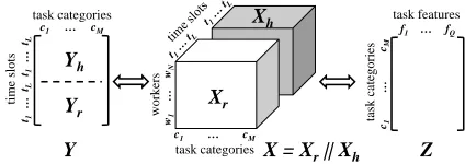
In this section, we build a worker-task-time tensor, Xr ∈ RN×M×L, based on the task-performing records in the most
recentLtime slots, to model the workers’ temporal prefer-ences for different categories of tasks, as illustrated in Fig-ure 2. The tensor consists of three dimensions, i.e., workers, task categories and time slots, and each entryXr(i, j, k) =e
denotes thei-th worker’s preferenceeon thej-th task cat-egory in time slotk (e.g.,10 : 00am−11 : 00am). Ob-viously, there exists missing entries in tensorXr. Once the
missing entries are inferred from other non-zero entries, we
task categories
w1
…
w
N
Xr Xh
X = Xr|| Xh
work
ers
c1 … cM
Yr Yh
Y
task categories
ti
m
e s
lot
s
t1
…
tL
t1
…
tL
c1 … cM
Z
task features
ta
sk
ca
te
gor
ie
s
f1 … fQ
c1
…
cM
Figure 2: Workers’ Temporal Preferences Modeling
can obtain all the workers’ preferences on any tasks in all theLtime slots.
However, the tensor is over sparse with large quantities of missing entries since only a few tasks can be performed by an individual worker in a short time period. It is not accu-rate enough to decomposeXrsolely based on its own
non-zero entries, so we introduce another tensor, Xh, based on
the historical task-performing records over a longer period of time (e.g., one month) aggregated by the corresponding time slots from1toL, which has the same structure asXr
shown in Figure 2. Clearly,Xh, representing the historical
task-performing patterns and workers’ long-term interests, is much denser thanXr. The error of supplementingXrcan
be greatly reduced by decomposingXrandXhtogether.
Context Matrix Construction
For more effective decomposition of the tensorXr, we also
construct another two matrices, i.e., time-task matrixY and task-feature matrixZ.
Time-task matrix. MatrixY consists ofYrandYh,
cap-turing the temporal correlation in terms of the distribution of task-performing conditions over different task categories, in which each row denotes a time slot and each column denotes a task category. In our work,YrandYhrespectively
repre-sent the recent and historical task-performing conditions in the same span of time of day. An entry of Yr ∈ RL×M,
Yr(k, j), represents the number of times that the tasks of
cat-egoryjhave been performed in time slotk. Consequently, the similarity of two different rows indicates the correlation of task-performing flows between two time slots. A worker may perform some similar tasks in time slottkandtgsince
these two time slots share a similar worker task-performing pattern. For instance, the task-performing behaviours of a worker might be similar at 10:00am-11:00am and 2:00pm-3:00pm, since she is likely to stay at her workplace and will-ing to perform some simple tasks, which do not affect her normal duties. Moreover,Yrcan be more dense as its entries
are aggregated from all the workers, therefore can help re-duce the error of decomposingXr.Yhhas the same structure
asYr, storing the number of times that the tasks with
differ-ent categories have been performed in differdiffer-ent time slots based on workers’ long term task-performing history.
Task-feature matrix. Matrix Z ∈ RM×Q captures the
and statistical information derived from historical worker profile. Each entryZ(j, f)ofZrepresents thef-th feature of task categoryj. The value ofZ(j, f)can be a real value which indicates the weight of the feature for the task cate-gory.
Tensor Decomposition and Completion
Due to our goal of modeling workers’ temporal preferences, we need to estimate the missing entries ofXr. A
straight-forward solution is leveraging tucker decomposition model, which is generally applied to higher-order principal compo-nent analysis (Kolda and Bader 2009). It decomposes a ten-sor into a core tenten-sor multiplied (or transformed) by a few matrices, based on the tensor’s non-zero entries. However, decomposingXr solely cannot get accurate enough results
since it is over sparse. For instance, when using one-day task-performing records in our dataset and setting1hour as a time slot, only 0.15% entries ofXrare non-zero.
To achieve a high accuracy of preference estimation, we combineXr andXh (i.e.,X = Xr||Xh) together and then
decomposeX ∈RN×M×2L with aid of the context
matri-cesY andZcollaboratively, which is shown in Figure 2. We utilize tucker decomposition to decomposeX into the mul-tiplication of a core tensor and three matrices as follows:
X ≈O×W W ×SS×T T (2)
whereO ∈ RdW×dS×dT is the core tensor and its entries
show the level of interaction between the three components; W ∈ RN×dW,S ∈
RM×dS, andT ∈
R2L×dT are the low
rank latent factor matrices for workers, task categories and time slots;dW,dS, anddT denote the dimensions of latent
factors.
The two context matrices can be factorized in the same way.Y ∈R2L×M can be factorized into the multiplication
of two matrices,Y =T ST, andZ ∈
RM×Qcan be
factor-ized into the multiplication of two matrices,Z =SV, where V ∈ RdS×Q is the low rank latent factor for task features
andQdenotes the dimension of task features. It is easy to see that tensorX shares matrixT withY and shares matrix SwithZ. Based on the knowledge of tensorXand two con-text matricesY andZ, we then decomposeX, in which the loss function is defined in Equation 3 to control the errors.
L(O, W, S, T , V) =1
2||X −O×WW×SS×TT|| 2+
λ1
2 ||Y −T S
T||2+λ2
2||Z−SV|| 2+
λ3 2 (||O||
2+||W||2+||S||2+||T||2+||V||2)
(3)
where||·||denotes the Frobenius norm,λ3
2(||O||
2+||W||2+
||S||2+||T||2+||V||2)is a regularization of penalties to
avoid over-fitting, and λ1,λ2 andλ3 are parameters
con-trolling the contribution of different parts during the decom-position. Note that the whole missing values are regarded as zeros. In this work, we apply gradient descent algorithm to minimize the loss function, and then recover the miss-ing values inX by multiplying the decomposed factors as
Xrec=O×W W×SS×T T.
Preference-aware Task Assignment
In the real-time scenario, where workers and tasks arrive dynamically and require immediate responses from an SC server, it is challenging to achieve the global optimal solu-tion for PTA problem. Since an SC server only has a local knowledge of the available tasks and workers at any instance of time instead of a global view of all the workers and tasks, we will optimize the task assignment locally at every time instance by maximizing the current assignments and give higher priorities to workers who show more preference on the tasks simultaneously. In the sequel, we propose three heuristics to solve our proposed problem including Basic, SpatialandTemporalheuristics.Preference-aware Task Assignment (PTA)
Algorithm
Taking workers’ preferences as the priority of task assign-ment, we propose a basic solution to solve the preference-aware task assignment problem by transforming it to Mini-mum Cost MaxiMini-mum Flow (MCMF) problem.
The MCMF is based on a flow network graph represen-tation of the task assignment problem for time instanceti,
in which the graph is represented by Gi = (V, E) with V corresponding to the set of vertices and E the set of edges. Specifically, given a set of online workers, Wi = {w1, w2, ...}, and a set of available tasks,Si ={s1, s2, ...},
at time instanceti, the number ofV and the number of E are
fixed to|Wi|+|Si|+ 2and|Wi|+|Si|+mrespectively,
wheremis the number of available assignments for all the workers. The available assignments for workerw(w∈Wi)
in time instanceti, denoted asAwi , should satisfy the
follow-ing three conditions:∀< w, s >∈Awi,s∈Si,
1)d(w.l, s.l)≤w.r, and
2)ti+t(w.l, s.l)≤s.p+s.φand
3) taskshas not been performed by workerw,
whered(w.l, s.l)is a given distance (e.g., Euclidean dis-tance) betweenw.lands.l, andt(w.l, s.l)is the travel time fromw.ltos.l. For the sake of simplicity, we assume all the workers share the same velocity, so the travel time cost be-tween two locations can be estimated with their Euclidean distance, e.g., t(w.l, s.l) = d(w.l, s.l). However, our pro-posed algorithms are not dependent on this assumption and can handle the case where workers are moving at differ-ent speeds. |Awi | denotes the number of available
assign-ments for worker w and thus we can sum the number of available assignments for all the workers to get m, i.e.,
m=P
w∈Wi|A
w i |.
For the vertices construction, each worker wj maps to a
vertex,vj, and each spatial taskskmaps to a vertex,v|Wi|+k.
In addition, two fictitious verticessrc(labeled asv0) anddst
(labeled asv|Wi|+|Si|+1) are created to represent the source
and destination respectively.
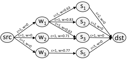
Figure 3 depicts an example of such network flow graph for three workers and six tasks at the same time instance. The corresponding edges are created using the following steps:
1) Edges associated fromsrcto the vertices mapped from Wiare created. For each edge connectingsrctovj(mapped
src
c=1, w=0 c=1, w=0.71dst
c=1, w=0.77 c=1, w=0.83
c=1, w=0
w
2w
1w
3s
3s
1s
2s
5Figure 3: Flow Network-based Graph
c(src, vj) = 1), since every worker is only capable of
per-forming one task at the current time instance. The cost of the these edges are set to0.
2) We generate|Si|edges connecting the vertices mapped
from Si todst, where the capacity of each edge is set to maxWsince every task is to be assigned to at mostmaxW workers. Same to edge(src, vj), the cost of these edges are
set to0.
3) Due to the spatial and temporal constraints, we add an edge from vj for every worker wj to the vertex v|Wi|+k
mapped from sk ∈ Si if sk can be assigned to wj, i.e., < wj, sk >∈Awij. For each edge(vj, v|Wi|+k), its capacity
is set to one and its cost (denoted byw(vj, v|Wi|+k)) can be
measured as the ratio between1and worker’s current pref-erences, i.e.,w(vj, v|Wi|+k) =
1
PT
wj(sk.c)+1.
The task assignment problem is now converted into a MCMF problem in the direct flow graph Gi from src to dst, which is to achieve the maximum flow of the graph while simultaneously minimize the cost. In our work, we use the Ford-Fulkerson algorithm (Kleinberg and Tardos 2005; Ford and Fulkerson 2009) to find the maximum flow of the network and then apply linear programming to minimize the cost of the flow (Kazemi and Shahabi 2012).
Spatial-weighted Preference-aware Task
Assignment (SPTA) Algorithm
The PTA does not consider travel cost between worker and her designated tasks, which is critical in SC as workers have to physically go to the locations of the tasks in order to per-form them. In our work, the travel cost between a workerw and a spatial tasks, denoted asd(w.l, s.l), is computed as a Euclidean distance between them. Due to the fact that a worker is more likely to accept nearby tasks (Ghinita, Gh-inita, and Shahabi 2014), we give higher priorities to the closer tasks by verifying worker preferences at time instance ti based on this heuristic. Given an online workerwand an
available tasksat time instanceti, the weighted preference
of workerwfor tasks, denoted byPw0(s), can be computed
as followed:
Pw0(s) =PT
w(s.c)·δ(w.l, s.l) (4)
δ(w.l, s.l) = 1−min(1, d(w.l, s.l)/w.r)
whereδ(w.l, s.l)is a function calculating the discount to the worker’s preference on the basis of her proximity to the task location. SPTA adapts PTA by calculating the weight of each
edge(vj, v|Wi|+k)connectingwjandskwith the weighted
preference, i.e.,w(vj, v|Wi|+k) =
1
Pw0(s)+1.
Temporal-weighted Preference-aware Task
Assignment (TPTA) Algorithm
This heuristic takes the temporal urgency of tasks into ac-count to prioritize tasks, based on the intuition that a task which is further away from its deadline is more likely to be performed in the future, and vice versa. As a result, near-deadline tasks should have higher priorities to be as-signed than others. Thus, in time instance ti, we define
the priority of a task sas the ratio between its remaining time and its vaild time, i.e., s.p+s.φ−ti
s.φ (s.p ≤ ti). TPTA
modifies PTA through setting the weight for each edge
(v|Wi|+k, v|Wi|+|Si|+1)connectingsk anddstwith the
pri-ority of a task, i.e.,w(v|Wi|+k, v|Wi|+|Si|+1) =
s.p+s.φ−ti
s.φ
(s.p≤ti).
Experiment
Experimental Setup
We use a check-in dataset from Twitter to simulate our prob-lem, which is a common practice in evaluation of SC plat-form (Deng, Shahabi, and Demiryurek 2013; Cheng et al. 2017; Dang, Nguyen, and To 2013). Since the original Twit-ter dataset does not contain category information of venues, we extract the category information associated with each venue from Foursquare with the aid of its API. The resulting dataset provides check-in data across USA except Hawaii and Alaska from September 2010 to January 2011, which includes locations of 62,462 venues and 61,412 users.
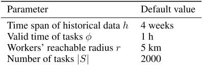
Table 1: Experiment Parameters
Parameter Default value
Time span of historical datah 4 weeks Valid time of tasksφ 1 h Workers’ reachable radiusr 5 km Number of tasks|S| 2000
Experimental Results
Performance of Temporal Preferences Modeling. We first evaluate the performance of workers’ temporal prefer-ences modeling phase and its impact to subsequent task as-signment. We set1hour as a time slot and use check-in data over a period ofxweeks (andx= 1,2,3,4with a default value of4) as historical data and check-in records of the day before as the recent data. The parameters (e.g.,λ1,λ2and
λ3) of loss function in tensor decomposition are set to0.01.
To evaluate the accuracy of estimating workers’ prefer-ences for tasks, we adopt the widely-used measures, Root Mean Square Error (RMSE) and Mean Absolute Error (MAE). We randomly remove20%of non-zero entries from the tensorXr, which are used as the testing set to evaluate
the inferred values, and the remaining80%are used as the training data. Then we introduce a baseline algorithm, Av-erage Value Filling (AVF) algorithm, which complements a missing entry with the average of all non-zero entries in the tensorX that belong to the corresponding time slot. More-over, we study the contribution of historical tensor (i.e.,Xh)
and context matrices (i.e.,Y andZ) for supplementing the missing entries. The methods are as followed:
1) AVF: Average value filling approach.
2) TD: Tensor decomposition approach that fills the miss-ing entries by decomposmiss-ing the tensorXrsolely based on its
own non-zero entries.
3) TD+H: Tensor decomposition approach that fills the missing entries by decomposing the tensor with historical data (i.e.,Xh).
4) TD+H+Y+Z (HCTD): Tensor decomposition approach that fills the missing entries by decomposing the tensor with historical data, time and task context.
Table 2 shows the evaluation results, in which AVF achieves the worst performance while HCTD performs best followed by TD+H and TD. That demonstrates our method, HCTD, can provide more accurate estimates for worker preferences by considering historical data, temporal features and correlation between different task categories.
We further evaluate the performance of TPM phase and its impact to subsequent task assignment by varying the size of historical data. In particular, for accuracy of pref-erence estimation, we compare the RMSE value of four dif-ferent approaches including AVF, TD, TD+H, HCTD. In ad-dition, we compare the assignment success rate of three dif-ferent task assignment algorithms: HCTD-based Task As-signment (HCTD-TA) algorithm, AVF-based Task Assign-ment (AVF-TA) algorithm, and MCTA (Dang, Nguyen, and To 2013) that solves task assignment problem by trans-forming it into maximum flow problem without
consider-Table 2: Performance of Different Methods for TPM
Methods MAE RMSE
AV F 0.2979 0.3384
T D 0.2671 0.3056
T D+H 0.2129 0.2406
T D+H+Y +Z(HCT D) 0.2054 0.2344
0.2 0.3 0.4
1 2 3 4
RMSE
Time span of historical data (week) AVF
TD TD+H HCTD
(a) RMSE
0 0.1 0.2 0.3 0.4
1 2 3 4
Assignment success rate
Time span of historical data (week) AVF-TA
MCTA HCTD-TA
(b) Assignment Success Rate
Figure 4: Performance of TPM: Effect ofh
ing workers’ preferences. When an SC server assigns a task sto workerw in a certain time instance (i.e.,ti), we
con-sider the assignment successful for wif there exists a task sharing the same category with the assigned task sin the worker’s task-performing list in the corresponding time slot
T (i.e., ti ∈ T). Thus we introduce Assignment Success
Rate (ASR), the ratio of successful assignments to the to-tal assignments for all workers in a certain time instance, to measure the accuracy of task assignment.
Effect of h. As shown in Figure 4a, naturally the accu-racy of all algorithms except TD gradually increases as the time span of historical data grows. The estimation accuracy of TD is not affected by the historical data since it decom-poses the tensor Xr solely without historical information.
AVF achieves the worst performance amongst these meth-ods. In addition, HCTD performs better than TD and TD+H, which testifies that the contributions of historical tensor and context matrices are effectiveness. In terms of task assign-ment success rate in Figure 4b, MCTA keeps constant since it does not consider worker preferences inferred from histor-ical data. In addition, HCTD-TA has increasing assignment success rate with varyinghdue to its increasing estimation accuracy for workers’ preferences, and it significantly out-performs the baseline algorithms for all values ofh, which confirms the superiority of our proposed algorithm.
Performance of Preference-aware Task Assignment.
Next we evaluate three different task assignment algo-rithms based on workers’ temporal preferences generated by HCTD: PTA, SPTA and TPTA algorithm. Two metrics are compared among these three methods: 1) CPU cost: the CPU time cost for finding the task assignment in a time in-stance; 2) ASR: Assignment Success Rate.
0 50 100 150 200
0.5 1 1.5 2 2.5
CPU time (ms)
Valid time of task (h) PTA
SPTA TPTA
(a) CPU Cost
0.2 0.3 0.4 0.5
0.5 1 1.5 2 2.5
Assignment success rate
Valid time of task (h) PTA
SPTA TPTA
(b) Assignment Success Rate
Figure 5: Performance of PTA: Effect ofφ
70 80 90 100 110 120 130
5 10 15 20
CPU time (ms)
Reachable radius of worker (km) PTA
SPTA TPTA
(a) CPU Cost
0.2 0.3 0.4 0.5
5 10 15 20
Assignment success rate
Reachable radius of worker (km) PTA
SPTA TPTA
(b) Assignment Success Rate
Figure 6: Performance of PTA: Effect ofr
of the edges in the flow network graph, which does not affect the computation complexity. Another observation is that the CPU cost of all the methods increases almost linearly withφ, since the number of available tasks in a time instance grows whenφgets longer, which in turn leads to more edges in the flow network graph of MFMC to be searched. The ASR val-ues of all methods are enhanced with the increasingφ(see Figure 5b) since a worker has more chance to be assigned her interested tasks whenφgrows longer. SPTA and TPTA perform worse than PTA since they take workers’ travel cost and tasks’ expiration time into account respectively, which weakens the impact of workers’ preferences on task assign-ment and leads to more inaccurate assignassign-ments.
Effect ofr.We also study the effects of the length of work-ers’ reachable radiusrby changing it from 5 km to 20 km. From Figure 6a we can see that, the CPU cost of all the methods has similar increasing trend whenrgrows. The rea-son behind it is that all the methods apply MFMC algorithm and more workers with greater reachable radius tend to have more available task assignments, which leads to more edges in the flow network graph of MFMC. As shown in Figure 6b, the assignment success rate of the three approaches has a growing tendency asris enlarged, with the similar reason of the effects of tasks’ valid time, i.e., the larger the work-ers’ reachable regions are, the more chance the SC server has to assign the workers their interested tasks.
Effect of|S|.To study the scalability of the proposed algo-rithms, we generate 5 datasets containing500to2500tasks by random selection from the original dataset in four hours (i.e., 10:00am–2:00pm) of a day. Besides the CPU cost and assignment success rate, we compare another two metrics among the three methods: 1) average travel cost of all the task assignments; 2) the total number of assigned tasks. As
0 20 40 60 80 100 120 140
500 1000 1500 2000 2500
CPU time (ms)
Number of tasks PTA
SPTA TPTA
(a) CPU Cost
0.1 0.2 0.3 0.4
500 1000 1500 2000 2500
Assignment success rate
Number of tasks PTA
SPTA TPTA
(b) Assignment Success Rate
0.6 1.0 1.4 1.8 2.2 2.6
500 1000 1500 2000 2500
Average travel cost (km)
Number of tasks PTA
SPTA TPTA
(c) Average Travel Cost
0 200 400 600 800 1000 1200
500 1000 1500 2000 2500
No. of assigned tasks
No. of tasks PTA SPTA TPTA
(d) Number of Assigned Tasks
Figure 7: Performance of PTA: Effect of|S|
expected, though the CPU cost increases as |S|increases, our proposed algorithms perform well in improving the task assignment success rate, which is demonstrated in Figure 7a and Figure 7b. Figure 7c shows the average travel cost of all algorithms decreases since there is a higher probability that an assigned task is closer to a worker in a task-dense area. Furthermore, we notice that SPTA outperforms both PTA and TPTA by an astounding margin (up to 42%), which demonstrates the effectiveness of the spatial (travel cost) heuristic. As depicted in Figure 7d, naturally the assign-ments of all approaches increase when more tasks exist. The figure also illustrates the superiority of TPTA compared with PTA and SPTA in terms of the number of assigned tasks (up to 40%), which stems from applying the temporal heuristic. Moreover, the impact of temporal heuristic becomes more significant as the number of tasks grows. The reason behind it is that with a larger number of tasks, more tasks are soon to expire, and thus, prioritizing the near-deadline tasks to be assigned becomes more effective.
Conclusion
Acknowledgements
The work is supported by the National Natural Science Foundation of China (Grant No. 61502324, 61532018, 61836007, 61832017 and 61872258). This work is also par-tially supported by Alibaba Innovation Research (AIR).
References
Alt, F.; Shirazi, A. S.; Schmidt, A.; Kramer, U.; and Nawaz, Z. 2010. Location-based crowdsourcing:extending crowd-sourcing to the real world. InNordiCHI, 13–22.
Ambati, V.; Vogel, S.; and Carbonell, J. 2011. Towards task recommendation in micro-task markets. InAAAI, 80–83. Buchholz, S., and Latorre, J. 2011. Crowdsourcing prefer-ence tests, and how to detect cheating. InISCA, 3053–3056. Cheng, P.; Lian, X.; Chen, L.; and Han, J. 2015a. Task assignment on multi-skill oriented spatial crowdsourcing. TKDE28(8):2201–2215.
Cheng, P.; Lian, X.; Chen, Z.; Fu, R.; Chen, L.; Han, J.; and Zhao, J. 2015b. Reliable diversity-based spatial crowdsourc-ing by movcrowdsourc-ing workers. VLDBJ8(10):1022–1033.
Cheng, P.; Lian, X.; Chen, L.; and Shahabi, C. 2017. Prediction-based task assignment in spatial crowdsourcing. InICDE, 997–1008.
Dang, H.; Nguyen, T.; and To, H. 2013. Maximum complex task assignment: Towards tasks correlation in spatial crowd-sourcing. InICPS, 77–81.
Deng, D.; Shahabi, C.; and Demiryurek, U. 2013. Maxi-mizing the number of worker’s self-selected tasks in spatial crowdsourcing. InSIGSPATIAL, 324–333.
Deng, D.; Shahabi, C.; and Zhu, L. 2015. Task matching and scheduling for multiple workers in spatial crowdsourcing. In SIGSPATIAL, 21.
Ford, L. R., J., and Fulkerson, D. R. 2009. Maximal flow through a network. Canadian Journal of Mathematics 8(3):399–404.
Ghinita, G.; Ghinita, G.; and Shahabi, C. 2014. A framework for protecting worker location privacy in spatial crowdsourcing. VLDBJ919–930.
Kazemi, L., and Shahabi, C. 2012. Geocrowd: Enabling query answering with spatial crowdsourcing. In SIGSPA-TIAL, 189–198.
Kleinberg, J., and Tardos, E. 2005. Algorithm design. Pren-tice Hall.
Kolda, T. G., and Bader, B. W. 2009. Tensor decompositions and applications. Siam Review51(3):455–500.
Li, Y.; Yiu, M.; and Xu, W. 2015. Oriented online route rec-ommendation for spatial crowdsourcing task workers.SSTD 137–156.
Song, T.; Tong, Y.; Wang, L.; She, J.; Yao, B.; Chen, L.; and Xu, K. 2017. Trichromatic online matching in real-time spatial crowdsourcing. InICDE, 1009–1020.
Tong, Y.; She, J.; Ding, B.; Chen, L.; Wo, T.; and Xu, K. 2016a. Online minimum matching in real-time spatial data: Experiments and analysis. VLDB9(12):1053–1064.
Tong, Y.; She, J.; Ding, B.; and Wang, L. 2016b. Online mobile micro-task allocation in spatial crowdsourcing. In ICDE, 49–60.
Tong, Y.; Wang, L.; Zhou, Z.; Ding, B.; Chen, L.; Ye, J.; and Xu, K. 2017. Flexible online task assignment in real-time spatial data. VLDB10(11):1334–1345.
Tong, Y.; Wang, L.; Zhou, Z.; Chen, L.; Du, B.; and Ye, J. 2018a. Dynamic pricing in spatial crowdsourcing: A matching-based approach. InSIGMOD, 773–788.
Tong, Y.; Zeng, Y.; Zhou, Z.; Chen, L.; Ye, J.; and Xu, K. 2018b. A unified approach to route planning for shared mo-bility. PVLDB11(11):1633–1646.
Yuen, M. C.; King, I.; and Leung, K. S. 2012. Task recom-mendation in crowdsourcing systems. InCrowdKDD, 22– 26.