High level feature extraction for the self-taught learning algorithm

(1)

R E S E A R C H

Open Access

High level feature extraction for the self-taught

learning algorithm

Konstantin Markov

1*

and Tomoko Matsui

2

Abstract

Availability of large amounts of raw unlabeled data has sparked the recent surge in semi-supervised learning research. In most works, however, it is assumed that labeled and unlabeled data come from the same distribution. This

restriction is removed in the self-taught learning algorithm where unlabeled data can be different, but nevertheless have similar structure. First, a representation is learned from the unlabeled samples by decomposing their data matrix into two matrices called bases and activations matrix respectively. This procedure is justified by the assumption that each sample is a linear combination of the columns in the bases matrix which can be viewed as high level features representing the knowledge learned from the unlabeled data in an unsupervised way. Next, activations of the labeled data are obtained using the bases which are kept fixed. Finally, a classifier is built using these activations instead of the original labeled data. In this work, we investigated the performance of three popular methods for matrix

decomposition: Principal Component Analysis (PCA), Non-negative Matrix Factorization (NMF) and Sparse Coding (SC) as unsupervised high level feature extractors for the self-taught learning algorithm. We implemented this algorithm for the music genre classification task using two different databases: one as unlabeled data pool and the other as data for supervised classifier training. Music pieces come from 10 and 6 genres for each database respectively, while only one genre is common for the both of them. Results from wide variety of experimental settings show that the self-taught learning method improves the classification rate when the amount of labeled data is small and, more interestingly, that consistent improvement can be achieved for a wide range of unlabeled data sizes. The best performance among the matrix decomposition approaches was shown by the Sparse Coding method.

Introduction

A tremendous amount of music-related data has recently become available either locally or remotely over networks, and technology for searching this content and retrieving music-related information efficiently is demanded. This consists of several elemental tasks such as genre classi-fication, artist identiclassi-fication, music mood classiclassi-fication, cover song identification, fundamental frequency estima-tion, and melody extraction. Essential for each task is the feature extraction as well as the model or classifier selec-tion. Audio signals are conventionally analyzed frame-by-frame using Fourier or Wavelet transform, and coded as spectral feature vectors or chroma features extracted for several tens or hundreds of milliseconds. However, it is an open question how precisely music audio should be coded depending on the task kind and the succeeding classifier.

*Correspondence: [email protected]

1Department of Information Systems, The University of Aizu, Fukushima, Japan Full list of author information is available at the end of the article

For the classification, classical supervised pattern recog-nition approaches require large amount of labeled data which is difficult and expensive to obtain. On the other hand, in the real world, a massive amount of musical data is created day by day and various musical databases are newly composed. There may be no labels for some databases and musical genres may be very specific. Thus, recent music information retrieval research has been increasingly adopting semi-supervised learning methods where unlabeled data are utilized to help the classifica-tion task. Common assumpclassifica-tion, in this case, is that both labeled and unlabeled data come from the same distri-bution [1] which, however, may not be easily achieved during the data collection. This restriction is alleviated in the transfer learning framework [2] which allows the domains, tasks, and distributions used in training and testing to be different. Utilizing this framework and the semi-supervised learning ideas, the recently proposed self-taught learning algorithm [3] appears to be a good candidate for the kind of music genre classification task

(2)

described above. According to this algorithm, first, a high-level representation of the unlabeled data is found in an unsupervised manner. This representation is assumed to hold some common structures appearing in the data such as curves, edges, or shapes for images or particular spec-trum changes for music. In other words, we try to learn some basic “building blocks” or high-level features rep-resenting the knowledge extracted from the unlabeled data. In practice, this is accomplished by decomposing the unlabeled data matrix into a matrix of basis vec-tors representing those “building blocks” and matrix of combination coefficients such that each data sample can be approximated by a linear combination of the basis vectors. The basis vectors matrix is often called a dic-tionary while the coefficients matrix is called an activa-tionsmatrix. There are various methods for this kind of matrix decomposition but most of them are based on the minimization of the approximation error, so the main difference between those methods lays in the used opti-mization algorithms. In this study, we investigated the performance of two recently proposed methods: the Non-negative Matrix Factorization (NMF) [4] and Sparse Cod-ing (SC) [5], as well as the classical Principal Component Analysis (PCA) [6] as approaches for learning the dictio-nary of basis vectors. Each method has its own advantages and drawbacks and some researchers have investigated their combinations by essentially adjusting the objective function to accommodate some constraints. Thus, the sparse PCA [7], the non-negative sparse PCA [8], and sparse NMF [4,9] have been introduced lately. However, in order to be able to do a fair comparison, we decided to use the original PCA and NMF rather than their sparse derivatives.

The next step of the self-taught learning algorithm involves transformation of the labeled data into new fea-ture vectors using the dictionary learned at the previous step. This is done using the same matrix factorization pro-cedure as before with the only difference that the basis vectors matrix is kept fixed and only the activation matrix is calculated. This way, each of the labeled data vectors is approximated by a linear combination of bases learned from a large amount of data. It is expected that the acti-vation vectors will capture more information than the original labeled data they correspond to, since additional knowledge encapsulated in the bases is being used. Finally, using labeled activation vectors as regular features, classi-cal supervised classifier is trained for the task at hand. In this work, we used the standard Support Vector Machine (SVM) classifier.

In our experiments, we utilized two music databases: one as unlabeled music data and the other for the actual supervised classiﬁcation task. We have published some preliminary experimental results on these databases [10,11], but this study provides a thorough investigation

and comparison of the three matrix decomposition meth-ods mentioned above.

Related studies

There are several studies where the semi-continuous learning framework has been used for music analysis and music information retrieval tasks. Based on a manifold regularization method, it has been shown that adding unlabeled data can improve the music genre classifica-tion accuracy rate [12]. This approach is later extended to include fusion of several music similarity measures which achieved further gains in the performance [13]. The so called “semi-supervised canonical density esti-mation” method was proposed for the task of automatic audio tag classification [14]. In this study, using the semi-supervised variants of the canonical correlation analysis and the kernel density estimation methods, authors have built a system for automatic music annotation with tags such as genre, instrumentation, emotion, style, rhythm, etc. According to the published results, adding unlabeled sound samples can improve both the precision and recall rates. In all these studies, although not explicitly stated, both the labeled and unlabeled data come from the same classes and have the same distribution. This is evident from the fact that the unlabeled data have been obtained by removing the labels from part of the data corpus used in the experiments. In the self-taught learning case, how-ever, the unlabeled data, though being of the same type, i.e., music, come from different classes (genres).

On the other hand, the non-negative matrix factoriza-tion and the sparse representafactoriza-tion methods have been applied in various music processing tasks, but in a stan-dard supervised learning scenario. An NMF based on Itakura-Saito divergence has been used for notes pitch estimation as well as decomposition of music into indi-vidual instrumental sounds [15]. In another study [16], a polyphonic music transcription is achieved by estimating the spectral proﬁle and temporal information for every note using NMF decomposition. Recent review of the sparse representations in audio and music [17] describes successful applications in such tasks as audio coding, denoising, blind source separation as well as automatic music transcription. In an experimental setup similar to our baseline, i.e., with no unlabeled data, high genre classi-ﬁcation performance has been reported using the so called Predictive Sparse Decomposition method [18].

(3)

unlabeled data is less than the feature vectors dimen-sion, the representation of the target data using these bases essentially becomes a dimensionality reduction. This observation is the basis of the self-taught dimension-ality reduction method [20], where special care is taken for the preservation of the target data structures in the origi-nal space in order to improve the k-means performance. In our system, labeled data dimension is also reduced, but the goal is to improve the supervised classiﬁcation accuracy.

The self-taught learning algorithm

A classiﬁcation task is considered with small labeled train-ing data setXl = {xl_i},i = 1,. . .,Mdrawn i.i.d. from an unknown distributionD. Eachxl_i ∈Rdis an input feature vector which is assigned a class labelyi∈Y = {1,. . .,C}.

In addition, a larger unlabeled training data set Xu =

{xu

i},xui ∈Rd,i=1,. . .,Nis available, which is assumed

only to be of the “same type” asXland may not be associ-ated with the class labelsYand distributionD. Obviously, in orderXuto help the classiﬁcation of the labeled data, it should not be totally diﬀerent or unrelated.

The main idea of the self-taught learning approach is to use the unlabeled samples to learn in an unsupervised way slightly higher level representation of the data [3]. In other words, to discover some hidden structures in the data which can be considered as basic building blocks. For example, if the data represent images, the algorithm would ﬁnd simple elements such as edges, curves, etc., so that the image can be represented in terms of these more abstract, higher level features. Once learned, this representation is applied to the labeled data Xl resulting in a new set of features which lighten the supervised learning task.

This idea is formalized as follows: each unlabeled data vectorxu_i is assumed to be generated as a linear combina-tion of some basis funccombina-tions:

xu i =

K

k=1

au_i,kbu_k (1)

where au_i,k ∈ R are the linear combination coeﬃcients speciﬁc toxu_i andbk ∈ Rd,k = 1,. . .,K are the basis functions. In the self-taught learning framework, these basis functions are considered as the data building blocks or the higher level features. Taking into account all the unlabeled training data, Equation (1) can be conveniently rewritten in the following matrix form:

Xu₌_Bu_Au ₍₂₎

where Xu ₌_[_xu

1,xu2,. . .,xuN]∈ Rd×N is a product of

two matricesBu = [bu₁,bu₂,. . .,bu_K]∈ Rd×K andAu = [au₁,au₂,. . .,au_N]∈ RK×N. Each columnau_i = {au_i,k}ofAu represents the coeﬃcient vector for data vectorxu_i. It is easy to see that Equation (2) essentially decomposes the training data matrixXu into two unknown matricesAu

andBuwhich are also often calledactivationmatrix and

dictionary(of bases) respectively. All the methods for ﬁnd-ingAu andBu discussed in the next section produce an approximative solution and thus, in practice, Equations (1) and (2) become:

xu i =

K

k=1

au_i,kbu_k+_iu (3)

Xu_≈_Bu_Au ₍₄₎

where _iu ∈ Rd _{is a Gaussian noise representing the}

approximation error.

After the dictionaryBuhas been learned from the unla-beled training dataXu, according to the self-taught learn-ing algorithm, this dictionary is used to obtain activations for the labeled dataXl. In other words, it is assumed that the labeled vectorsxl_i can also be represented as a linear combination of some basis functions and particularly the basis vectorsbu_k:

xl i=

K

k=1

al_i,kbu_k+_il (5)

Xl_≈_Bu_Al ₍₆₎

where Al =[al₁,al₂,. . .,al_M]∈ RK×M is the activation matrix corresponding to the labeled data. We can con-sider these activations as a new representation ofXland the whole procedure as a non-linear mapping or transfor-mation of vectorsxl_i ∈ Rd into vectorsal_i ∈ RK. Note that in the case whend>K, this transformation involves dimension reduction as well. Next, we can assign origi-nal class labelsyito eachal_i and thus obtain new labeled

training data which we can use to build any appropriate classifier in the traditional supervised manner. In other words, instead of the original training dataXl, we use the set of activationsAl= {al_i}as feature vectors for our clas-sification task. This exchange is justified when the amount of original labeled training data is too small for reliable model estimation. Although the size of the new training setAl is the same, the new feature vectors may contain more information about the underlying classes because they are obtained using the higher level features, i.e., the basis functions, learned from a much bigger pool of data. This can be considered as a transfer of structural informa-tion or knowledge from one set of data to another under the reasonable assumption that both the data sets share the same or similar higher level features.

The whole self-taught learning algorithm can be sum-marized into the following steps:

(4)

Step 2. Obtain activation vectorsal_ifor each labeled train-ing vectorxl_iusing the dictionary learned at Step 1. Step 3. Use activation vectorsal_i as new labeled features to train standard supervised classiﬁer.

Step 4. Transform each test vector into an activation vec-tor in the same way as the training data at Step 2 and apply the classiﬁer to obtain its label.

Data matrix decomposition and feature transformation methods

The general approach for ﬁnding the solution, i.e.,Auand

Bu_{, for the Equations (3) or (4) is the minimization of the}

squared approximation error:

min a,b

N

i=1 xu

i − K

k=1

ai,kbk 22 (7)

which in the matrix form can be expressed by the Frobe-nius norm:

Au_,_Bu₌_{arg min}

A,B DF(X

u_AB₎₌ 1

2 X

u₋_BA2 F (8)

Since there is no unique solution to the above opti-mization problem, the different miniopti-mization approaches described in this section result in solutions with different properties and, consequently, different performance.

For the labeled data transformation into activation vec-tors, similar optimization objective is used:

al

i=arg min_a xli− K

k=1

akbuk22 (9)

where al_i is the activation vector corresponding to xl_i. It is easy to see that this is a sub-task of the optimization of Equation (7) and can be solved using the same or even simpler method.

Principal Component Analysis (PCA)

The PCA [6] is a popular data-processing and dimension-reduction technique, with numerous applications in engi-neering, biology, and social science. It identiﬁes a low dimensional subspace of maximal variation within the data in an unsupervised manner. It is not diﬃcult to show that the following function [21]:

J(K)= N

i=1

m+ K

k=1 ai,kek

−xi

2

(10)

wheremis the data mean, is minimized when the vectors

ek are the K eigenvectors of the data covariance matrix

having largest eigenvalues, and the coeﬃcients ai are

calledprincipal components. Assuming that our unlabeled

data are mean normalized, i.e.,m = 0, and comparing

this equation with Equation (7) we see that the eigenvec-tors and the principal components correspond to the basis functionsbu_kand activationsau_i respectively.

The standard way of performing PCA is to do a singular value decomposition (SVD) of the data matrix:

Xu₌_Wuu_[_Vu_]T ₍₁₁₎

whereWu is the eigenvectors matrix, i.e., the dictionary, andPu=u[Vu]Tis the matrix of principal components, i.e., the activations matrix.

In this case, the labeled data transformation, i.e., Equation (9), is simpliﬁed to:

al

i=[Wu]Txli (12)

which together with the SVD procedure required for

ﬁnd-ing the matrix Wu makes the PCA approach very easy

to implement and computationally inexpensive way of calculating the high level features for the self-taught learn-ing algorithm. However, compared to the other matrix decomposition methods, the PCA has several limitations. First, as can be seen from the above equation, the PCA results in linear feature extraction, i.e., activations are just linearly transformed input data. Other methods, such as sparse coding, can produce features which are inherently a non-linear function of the input. Second, the dictionary size cannot be bigger than the data dimension because the eigenvectors are assumed to be orthogonal. Finally, it is diﬃcult to think of the eigenvectors as building blocks or higher level structures of the data.

Non-negative Matrix Factorization (NMF)

In this case, to learn the higher level representation, we use the non-negative matrix factorization method. It

decomposes the unlabeled data matrix Xu _{into a}

prod-uct of two matricesWu ₌_[_wu

1,wu2,. . .,wun]∈ Rd×K and Hu ₌_[_hu

1,hu2,. . .,huK]∈ RK×N having only non-negative

elements. The decomposition is approximative in nature, so:

Xu_≈_Wu_Hu ₍₁₃₎

or equivalently in a vector form:

xu i ≈

K

k=1

hu_i,kwu_k (14)

where Hu is the mixing matrix corresponding to the

activations matrixAu andWu corresponds to the bases matrixBu of Equation (4). Since only additive combina-tions of these bases are allowed, the non-zero elements of

Wu_and_Hu_{are all positive. Thus, in such decomposition}

(5)

In contrast to the sparse coding method, the NMF does not assume explicitly or implicitly sparseness or mutual statistical independence of components. However, some-times it can produce sparse decompositions [22].

For ﬁnding W andH, the most frequently used cost

functions are the Square Euclidean distance expressed by the Frobenius norm:

DF(XWH)=

1

2 X−WH

2

F (15)

which is optimal for Gaussian distributed approximation error, and the generalized Kullback-Leibler divergence:

DKL(XWH)=

i,j

xijlog

xij

[WH]_ij

−xij+[WH]ij

.

(16)

Although both functions are convex in W and H only,

they are not convex in both variables together. Thus, we can only expect the maximization algorithm to ﬁnd a local minimum. A good compromise between speed and ease of implementation have been proposed in [23] and is known as the multiplicative updates algorithm. It consists of iterative application of the following update rules:

hij←hij

[WT_X_] ij

[WT_WH_]_ij (17)

wij←wij

[XHT_] ij

[WHHT_]_ij (18)

when Frobenius norm (Equation (15)) is chosen as objec-tive function. Another popular optimization method is the alternating least squares (ALS) algorithm where simpler objective is solved by ﬁxing one of the unknown matri-ces and then solving again with the other matrix held ﬁxed. The ALS algorithm, however, does not guarantee convergence to a global minimum or even to a station-ary point. Some other approaches such as the Projected Gradient or Quasi-Newton method have been shown to give better results. An excellent and deep descrip-tion of the NMF and its optimizadescrip-tion methods is given in [4].

After learning the basis vectorswu_i from the unlabeled training dataXuwe use them to obtain activations for the labeled dataXl. The new labeled features are computed by solving Equation (9) which in the case of NMF is:

hl

i=arg min_h xli− K

k=1

hkwuk22 (19)

This is a convex least squares task which is the same as the optimization of (15) with ﬁxed baseswk and can be solved in the by using the update rule just for hij, i.e.,

Equation (17).

Sparse Coding (SC)

To learn the higher level representation with a sparse cod-ing method, we can add a sparsity constraint to the objec-tive function of Equation (7). Given the unlabeled data set Xu_{, the following optimization procedure is deﬁned:}

min a,b

N

i=1 xu

i − K

k=1

ai,kbk22+βai1 (20)

subject tobk2≤1, k=1,. . .,K

where basis vectorsbk ∈ Rd_,_k ₌ _1,_{. . .}_,_K _and

activa-tionsai ∈ RK_,_i ₌ _1,_{. . .}_,_N _{are subject to optimization.}

The parameterβ controls the sparsity level and is usu-ally tuned on a development data set. The ﬁrst term of the above objective tries to represent each data vector as a linear combination of the basesbk with weights given by the corresponding activations. The second term, on the other hand, tries to reduce theL1norm of the

activa-tion vectors, thus making them sparse. The optimizaactiva-tion problem is convex only in terms of basis vectors or activa-tions alone and these sub-problems are solved iteratively by alternatingly holing ai or b_k ﬁxed. For learning the bases, the problem is a least squares optimization with quadratic constraints which in general is solved using gra-dient descent or convex optimization approaches such as the quadratically constrained quadratic programming (QCQP). For the activations, the optimization problem is a convex L1-norm regularized least squares problem

and the possible solutions include generic QP solvers, least angle regression (LARS) [24] or grafting [25]. In our experiments, however, we used the more eﬃcient feature-sign search algorithm [26]. It is based on the fact that if the sign ofai,kis known, then the optimization problem is

reduced to a standard, unconstrained QP problem, which can be solved analytically.

After learning the basis vectorsbu_k from the unlabeled

training data Xu as described above, we use them to

obtain activations for the labeled dataXl _{by solving the}

following optimization problem:

al

i=arg min_a xli− K

k=1

akbu_k22+βa1 (21)

This is the same as the optimization problem of Equation (20) with ﬁxed basesb_kand can be solved using the same feature-sign search algorithm. Vectorsal_i are sparse and approximate labeled data xl_i as a linear combination of the bases which, however, are learned using the unlabeled dataXu.

Experiments

(6)

All data sets, signal processing and classiﬁcation meth-ods are common to all the matrix decomposition methmeth-ods described in the previous section.

Databases

As unlabeled database we used the GTZAN collection of music [27]. It consists of 1000 30 s audio clips, each belonging to one of the following ten genres: Classical, Country, Disco, Hip-Hop, Jazz, Rock, Blues, Reggae, Pop and Metal. There are 100 clips per genre and all of them have been down-sampled to 22050 Hz. The other database which we used as labeled data is the corpus used in the ISMIR 2004 audio contest [28]. It contains of 729 whole tracks for training, but since the number of tracks per genre is non-uniform, the original nine genres are usually mapped into the following six classes: Classical, Electronic, Jazz-Blues, Metal-Punk, Rock-Pop and World. Another 729 tracks are used for testing. Note that the only common genre between the two databases is the “Classical” genre.

Audio data from both databases are divided into 5 s pieces which were further randomly selected in order to make several training sets with diﬀerent amount of data, keeping the same number of such pieces per genre. Table 1 summarizes the contents of the training data sets we used in our experiments. For example, set GT-50 has 50 randomly selected 5 s pieces per genre, 500 pieces in total or 0.69 h of music from the GTZAN database. In con-trast, IS-20 is a data set from the training part of the ISMIR 2004 corpus consisting of 20 pieces per genre or 120 pieces in total. All sets are constructed in such way that each larger set contains all the pieces from the smaller set. There is only one test set and it consists of 250 pieces per genre randomly selected from the ISMIR 2004 test tracks.

Audio signal preprocessing

When it comes to feature extraction for music infor-mation processing, in contrast to the case of speech where the MFCC is dominant, there exists wide variety of approaches—from carefully crafted multiple music spe-ciﬁc tonal, chroma, etc. features to single and simple “don’t care about the content” spectrum. In our experiments, we used spectral representation tailored for music signals,

Table 1 Data sets used in the experiments

GTZAN database ISMIR 2004 database

Set Pieces Hours Set Pieces Hours

GT-50 500 0.69 IS-20 120 0.17

GT-100 1000 1.39 IS-50 300 0.42

GT-250 2500 3.47 IS-100 600 0.83

GT-500 5000 6.95 IS-250 1500 2.08

Table 2 PCA baseline classiﬁcation accuracy (%)

Training Dictionary size K

Set 100 200 300 500

IS-20 38.5 36.8 36.5 35.6

IS-50 43.5 41.8 41.8 41.7

IS-100 54.3 52.3 53.3 53.0

IS-250 56.0 56.3 56.6 57.3

Bases are learned from the labeled ISMIR training data.

such as the Constant-Q transformed (CQT) FFT spec-trum. The CQT can be thought of as a series of logarith-mically spaced ﬁlters having constant center frequency to bandwidth ratio, i.e.,

fk fk =

Q (22)

whereQis known as the transform’s “quality factor”. The main property of this transform is the log-like frequency scale where the consecutive musical notes are linearly spaced [29].

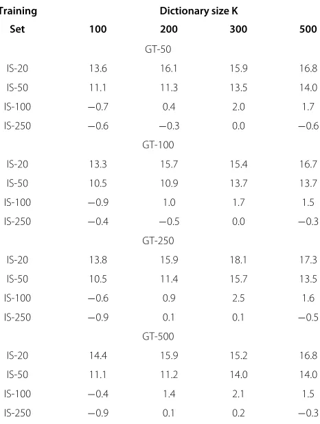
Table 3 Absolute improvement (%) wrt the PCA baseline when bases are learned from the unlabeled GT data sets

Set 100 200 300 500

GT-50

IS-20 13.6 16.1 15.9 16.8

IS-50 11.1 11.3 13.5 14.0

IS-100 −0.7 0.4 2.0 1.7

IS-250 −0.6 −0.3 0.0 −0.6

GT-100

IS-20 13.3 15.7 15.4 16.7

IS-50 10.5 10.9 13.7 13.7

IS-100 −0.9 1.0 1.7 1.5

IS-250 −0.4 −0.5 0.0 −0.3

GT-250

IS-20 13.8 15.9 18.1 17.3

IS-50 10.5 11.4 15.7 13.5

IS-100 −0.6 0.9 2.5 1.6

IS-250 −0.9 0.1 0.1 −0.5

GT-500

IS-20 14.4 15.9 15.2 16.8

IS-50 11.1 11.2 14.0 14.0

IS-100 −0.4 1.4 2.1 1.5

(7)

Table 4 NMF baseline classiﬁcation accuracy (%)

Set 100 200 300 500

IS-20 52.7 53.1 54.2 54.5

IS-50 54.4 55.8 56.3 57.2

IS-100 52.7 54.0 55.3 56.9

IS-250 54.2 55.8 56.6 57.5

The CQT transform is applied to the FFT spectrum vec-tors computed from 23.2 ms (512 samples) frames with 50 % overlap in a way that there are 12 Constant-Q fil-ters per octave resulting in a filter-bank of 89 filfil-ters which covers the whole bandwidth of 11025 Hz. The filter-bank outputs of 20 consecutive frames are

fur-ther stacked into a 1780 (89 × 20) dimensional

super-vector which is used in the experiments. This is the same as to have a 20 frame time-frequency spectrum image. There is a overlap of 10 frames between such two consecutive spectrum images. This way, each 5 s music piece is represented by 41 spectrum images or super-vectors.

Table 5 Absolute improvement (%) wrt the NMF baseline when bases are learned from the unlabeled GT data sets

Set 100 200 300 500

GT-50

IS-20 ₋1.53 0.27 ₋0.93 ₋0.54

IS-50 ₋0.47 1.13 1.20 1.33

IS-100 0.40 −0.07 −0.33 0.33

IS-250 −1.07 0.00 0.20 0.00

GT-100

IS-20 −1.06 −0.2 0.07 −0.80

IS-50 −0.67 1.20 1.67 1.20

IS-100 0.40 −0.40 −0.33 0.46

IS-250 −0.20 −0.33 0.67 0.00

GT-250

IS-20 −2.53 −0.26 0.47 −0.34

IS-50 −0.93 1.60 1.67 1.13

IS-100 −0.06 0.27 0.47 −0.80

IS-250 −0.27 0.00 0.07 0.00

GT-500

IS-20 −3.06 −0.93 0.27 −0.94

IS-50 −1.67 1.87 1.33 1.06

IS-100 −0.40 −0.33 −0.13 −0.74

IS-250 −0.87 −0.40 −0.67 0.00

Table 6 SC baseline classiﬁcation accuracy (%)

Set 100 200 300 500

IS-20 52.5 52.4 51.5 54.1

IS-50 56.3 58.6 58.9 60.9

IS-100 57.0 58.9 60.1 62.3

IS-250 57.4 59.9 61.7 64.0

Bases learning

For each data set given in Table 1 we learned several basis vector sets or dictionaries. The sets sizesKare: 100, 200, 300 and 500. Contrary to the conventional sparse coding scheme, where the dictionary size is much bigger than the vectors dimension (for over-complete represen-tation), in our case we in fact do dimension reduction. This is motivated by the fact that our super-vectors are highly redundant and that the basis vectors actually repre-sent higher level spectral image features, not just arbitrary projection directions.

Before bases learning, all the feature vectors from the corresponding GTZAN data set are pooled together and

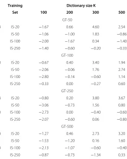
Table 7 Absolute improvement (%) wrt the SC baseline when bases are learned from the unlabeled GT data sets

Set 100 200 300 500

GT-50

IS-20 ₋1.67 0.66 4.60 2.54

IS-50 ₋1.06 ₋1.00 1.83 ₋0.86

IS-100 −2.00 −1.67 0.34 −1.40

IS-250 −1.40 −0.60 −0.20 −0.33

GT-100

IS-20 −0.67 0.40 3.40 1.94

IS-50 −2.06 −0.06 1.76 2.74

IS-100 −2.80 −0.14 −0.60 1.14

IS-250 −0.33 0.00 −0.27 0.60

GT-250

IS-20 −0.80 0.20 3.80 3.67

IS-50 −3.06 −0.73 1.56 0.80

IS-100 −2.73 0.00 −0.40 −0.60

IS-250 −2.07 −0.60 0.06 −0.80

GT-500

IS-20 −1.27 0.46 2.73 3.20

IS-50 −1.53 −1.20 0.16 1.60

IS-100 −2.13 −1.07 −0.60 −0.40

(8)

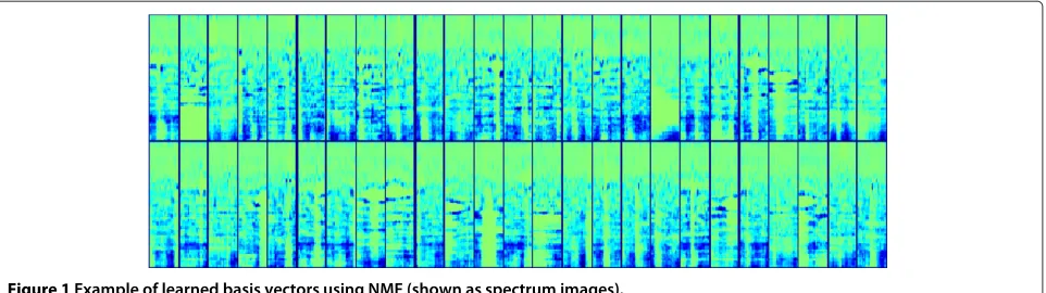
Figure 1Example of learned basis vectors using NMF (shown as spectrum images).

randomly shuﬄed. Then, each of the matrix decompo-sition method is applied and the respective dictionaries learned.

Supervised classification

After all labeled training data, i.e. sets 20, 50, IS-100 and IS-250, have been transformed into activation vectors for each dictionary learned from each unlabeled data set, we obtained in total 64 (4 labeled data sets × 4 dictionary sizes×4 unlabeled data sets) labeled train-ing data sets. Then, ustrain-ing the LIBSVM tool, we learned 64 SVM classifiers each consisting of 6 SVMs trained in one-versus-all mode. The SVM input vectors were lin-early scaled to fit the [ 0, 1] range. For the sparse coding method, this significantly reduces vectors sparsity, but it is tolerable since our goal is not the sparse represen-tation itself. Linear kernel was used as distance mea-sure and the SVMs were trained to produce probabilistic outputs.

During testing, each 5 s musical piece represented by 41 feature (activation) vectors is considered as a sam-ple for classification. Outputs of all genre specific SVMs are aggregated (summed in the log domain) and the label of the maximum output is taken as the classification result.

In order to assess the eﬀect of the self-taught learn-ing, we need performance comparison with a system build under the same conditions but without unlabeled data. We will refer to this system as baseline. In this case, the basis vectors are learned using labeled training dataXl_instead

of the unlabeled Xu_{. Then, the activations are obtained}

in the same way as if the bases were learned from the unlabeled data.

Results using PCA

Table 2 shows the baseline results in terms of genre clas-siﬁcation accuracy for each data set IS-20, IS-50, IS-100 and IS-250 with respect to the number of eigenvectors used, i.e., dictionary sizeK. As can be seen, performance improves with the data set size, but doesn’t change much with respect to the activation features dimension. This suggests that the input data are highly redundant and that the information captured by the eigenvectors is propor-tional to the data set size.

Using larger amount of data to obtain the eigenvectors through the self-taught learning algorithm signiﬁcantly improves the results for the poorly performing data sets IS-20 and IS-50 as evident from the Table 3. In this table, the absolute improvement with respect to the base-line accuracy is shown in four sub-tables, one for each of the unlabeled data sets GT-50, GT-100, GT-250 and GT-500. It is interesting to notice that the improvement due to the unlabeled data doesn’t change with the data set size.

Results using NMF

The same set of experiments was done with the non-negative matrix factorization method. Results summa-rized in Tables 4 and 5 correspond to those for PCA which we described in the previous section.

(9)

Table 8 Some main diﬀerences and similarities of the PCA, NMF and SC methods

PCA NMF SC

Number of bases Less or same Less, same or more Less, same or more

wrt input dimension

Bases orthogonality Yes No No

Bases learning Analytic Iterative Iterative

Data representation Linear Non-linear Non-linear

Data sign Any Positive Any

Sparsity No Uncontrollable Adjustable

We can see that the baseline performance is much better than the PCA baseline, especially for the small data sets IS-20 and IS-50. Application of the self-taught learning, however, did not result in such deﬁnite improvement as in the case of PCA. In average, the unlabeled data helped for the middle range data sets, IS-50 and IS-100 when the dictionary size was 200 or 300.

Results using sparse coding

The last two tables, Tables 6 and 7, show the correspond-ing results for the sparse codcorrespond-ing method. As in the NMF, the baseline performance is much better than the PCA, and in some cases even better. The SC approach achieved the best baseline accuracy of 64 %.

As for the self-taught learning eﬀect, we can see clear performance improvement for the small data sets IS-20 and IS-50, though not as big as in the PCA case.

Discussion

To some extend, the results presented in the previous section highlight the strengths and drawbacks of each of the matrix decomposition methods we used in our experiments. The PCA is easy to implement and com-putationally not expensive, but it fails to capture enough

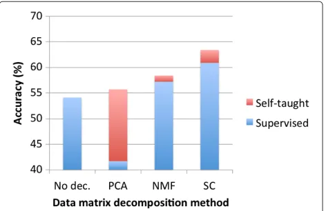
Figure 3Genre classification results using the IS-20 data set for training in both the supervised and self-taught learning scenarios.

structural information from the data and shows the low-est absolute classiﬁcation rate. The drawbacks of the PCA are well known and include the lack of sparseness, i.e., activations are linear combinations of the input data, dif-ﬁculty to interpret the results in terms of high level data shapes, and the upper limit on the number of achievable basis vectors.

On the other hand, the NMF and sparse coding meth-ods have iterative solutions which may become compu-tationally challenging for big data sets, but they provide non-linear labeled data transformation albeit with diﬀer-ent degree of sparsity. In the standard NMF method it is not possible to control the sparseness and depending on the data it can be quite low. In contrast, the sparse coding approach allows the sparseness to be adjusted (to some degree of course, since if set too high it may lead to sta-bility and numerical issues) and optimized with respect to the data. It is expected that higher degree of sparseness forces more information to be captured by the basis vec-tors which is essential for the success of the self-taught learning algorithm. This is also evident from the visual inspection of the learned basis vectors using NMF and sparse coding shown in Figures 1 and 2, respectively. It is apparent that the bases learned by the SC exhibit

(10)

clearer spectrum shapes with higher diversity than the NMF bases. Some of the main diﬀerences and similarities of all the three methods are summarized in Table 8.

In order to evaluate the self-taught learning algorithm itself, we obtained genre classification accuracy using the initial set of 1780 dimensional feature vectors, i.e., with-out any matrix decomposition and transformation, and a SVM classifier. The results of this evaluation are shown in Figures 3, 4, 5, and 6 for each training set 20, IS-50, IS-100, and ID-2IS-50, respectively, compared with the corresponding results obtained using each of the PCA, NMF, and SC data matrix decomposition methods for their best conditions. The improvement from the self-taught learning with unlabeled data is added to each of the bars in different color. Clearly, even in the regular super-vised setup, NMF and SC can produce some gain in the classification performance. In total, including the effect of the unlabeled data usage, the improvement especially for small target data sizes, is quite substantial.

Conclusion

In this study, we investigated the performance of several matrix decomposition methods, such as PCA, NMF and sparse coding when applied for high level feature extrac-tion in the self-taught learning algorithm with respect to the music genre classiﬁcation task. Results of the exper-iments conducted under various conditions showed that the sparse coding method outperforms the PCA in abso-lute recognition accuracy and the NMF in terms of relative improvement due to the knowledge extracted from the unlabeled data.

As for the self-taught learning algorithm itself, the results show that it achieves its purpose, i.e., to improve the performance when the amount of labeled data is small. Experiments also suggested that this improvement in not sensitive to the size of unlabeled data set.

Competing interests

The authors declare that they have no competing interests.

Author details

1_{Department of Information Systems, The University of Aizu, Fukushima,}

Japan.2_{Department of Statistical Modeling, Institute of Statistical}

Mathematics, Tokyo, Japan.

Received: 31 October 2012 Accepted: 6 March 2013 Published: 9 April 2013

References

1. K Nigam, A McCallum, S Thrun, T Mitchell, Text classiﬁcation from labeled and unlabeled documents using EM. Machine Learning.39(2–3), 103–134 (2000)

2. S Pan, Q Yang, A survey on transfer learning. IEEE Trans. Knowledge Data Eng.22(10), 1349–1359 (2010)

3. R Raina, A Battle, H Lee, B Packer, A Ng, inProceedings of International Conference on Machine Learning. Self-taught learning: transfer learning from unlabeled data (New York, NY, 2007), pp. 759–766

4. A Cichocki, R Zdunek, A Phan Huy, S Amari,Nonnegative Matrix and Tensor Factorizations. (John Wiley & Sons, UK, 2009)

5. B Olshausen, D Field, Field, Emergence of simple-cell receptive ﬁeld properties by learning a sparse code for natural images. Nature.381(13), 607–609 (1996)

6. I Jolliﬀe,Principal Component Analysis. (Springer Verlag, New York, 1986) 7. H Zou, T Hastie, R Tibshirani, Sparse principal component analysis. Journal

of Computational and Graphical Statistics.15(2), 265–286 (2006) 8. R Zass, A Shashua, inProceedings of the Twentieth Annual Conference on

Neural Information Processing Systems. Nonnegative sparse PCA (Vancouver, British Columbia, 2006), pp. 1561–1568

9. T Virtanen, Monaural sound source separation by non-negative matrix factorization with temporal continuity and sparseness criteria. IEEE Trans. Audio Speech Lang. Process.15(3), 1066–1074 (2007)

10. K Markov, T Matsui, inProceedings of IEEE International Conference on Acoustics, Speech, Signal Processing. Music genre classiﬁcation using self-taught learning via sparse coding (Kyoto, 2012), pp. 1929–1932 11. K Markov, T Matsui, inProceedings of IEEE International Workshop on

Machine Learning for Signal Processing. Nonnegative matrix factorization based self-taught learning with application to music genre classiﬁcation (Santander, Spain, 2012), pp. 1–5

12. Y Song, C Zhang, S Xiang, inProceedings of IEEE International Conference on Acoustics, Speech, Signal Processing. Semi-supervised music genre classiﬁcation (Honolulu, Hawaii, 2007), pp. 729–732

13. Y Song, C Zhang, Content-based information fusion for semi-supervised music genre classiﬁcation. IEEE Trans. Multimedia.10(1), 145–152 (2008) 14. J Takagi, Y Ohishi, A Kimura, M Sugiyama, M Yamada, H Kameoka, in

(11)

Processing. Automatic audio tag classiﬁcation via semi-supervised canonical density estimation (Prague, 2011), pp. 2232–2235

15. C Fevotte, N Bertin, J Durrieu, Nonnegative matrix factorization with the Itakura-Saito divergence: with application to music analysis. Neural Computation.21(3), 793–830 (2009)

16. P Smaragdis, J Brown, inProceedings of IEEE Workshop on Applications of Signal Processing to Audio and Acoustics. Non-negative matrix factorization for polyphonic music transcription (New Paltz, USA, 2003), pp. 177–180 17. M Plumbley, T Blumensath, L Daudet, R Gribonval, M Davies, Sparse

representations in audio and music: from coding to source separation. Proc. IEEE.98(6), 995–1005 (2010)

18. M Henaﬀ, K Jarrett, K Kavukcuoglu, Y LeCun, inProceedings of the 12th International Society for Music Information Retrieval Conference. Unsupervised learning of sparse features for scalable audio classiﬁcation (Miami, FL, 2011)

19. W Dai, Q Yang, GR Xue, Y Yu, inProceedings of International Conference on Machine Learning. Self-taught clustering (Helsinki, 2008), pp. 200–207 20. X Zhu, Z Huang, Y Yang, HT Shen, C Xu, J Luo, Self-taught dimensionality

reduction on the high-dimensional small-sized data. Pattern Recognition. 46(1), 215–229 (2013)

21. R Duda, P Hart, D Stork,Pattern Classification, 2nd edn. (John Wiley & Sons, USA, 2001)

22. D Lee, H Seung, Learning the parts of objects by non-negative matrix factorization. Nature.401(6755), 788–791 (1999)

23. D Lee, H Seung, inProceedings of Conference on Neural Information Processing Systems. Algorithms for non-negative matrix factorization (Denver, CO, 2000), pp. 556–562

24. B Efron, T Hastie, I Johnstone, R Tibshirani, Least angle regression. The Annals of Statistics.32(2), 407–499 (2004)

25. S Perkins, J Theiler, inProceedings of International Conference on Machine Learning. Online feature selection using grafting (Washington, DC, 2003), pp. 592–599

26. H Lee, A Battle, R Raina, A Ng, inProceedings of the Twentieth Annual Conference on Neural Information Processing Systems. Eﬃcient sparse coding algorithms (Vancouver, British Columbia, 2006), pp. 801–808 27. G Tzanetakis, P Cook, Musical genre classiﬁcation of audio signals. IEEE

Trans. Acoustics, Speech and Language Processing.10(5), 293–302 (2002) 28. P Cano, E Gomes, F Gouyon, P Herrera, M Koppenberger, B Ong, X Serra, S

Streich, N Wack, ISMIR 2004 Audio Description Contest. Tech. Rep. MTG-TR-2006-02, Universitat Pompeu Fabra (2006)

29. C Schoerkhuber, A Klapuri, inProceedings of the 7th. Sound and Music Computing Conference. Constant-Q transform toolbox for music processing, (Barcelona, 2010)

doi:10.1186/1687-4722-2013-6

Cite this article as:Markov and Matsui:High level feature extraction for the self-taught learning algorithm.EURASIP Journal on Audio, Speech, and Music Processing20132013:6.

Submit your manuscript to a

journal and beneﬁ t from:

7 Convenient online submission

7 Rigorous peer review

7 Immediate publication on acceptance

7 Open access: articles freely available online 7 High visibility within the ﬁ eld

7 Retaining the copyright to your article