R E S E A R C H
Open Access
Singular Value Homogenization: a simple
preconditioning technique for linearly
constrained optimization and its potential
applications in medical therapy
Dan-Daniel Erdmann-Pham
1, Aviv Gibali
2*, Karl-Heinz Küfer
3and Philipp Süss
3*Correspondence:
2Mathematics Department, ORT
Braude College, Karmiel, 21982, Israel
Full list of author information is available at the end of the article
Abstract
A wealth of problems occurring naturally in the applied sciences can be reformulated as optimization tasks whose argument is constrained to the solution set of a system of linear equations. Solving these efficiently typically requires computation of feasible descent directions and proper step sizes - the quality of which depends largely on conditioning of the linear equality constraint. In this paper we present a way of transforming such ill-conditioned problems into easily solvable, equivalent formulations by means of directly changing the singular values of the system’s associated matrix. This transformation allows us to solve problems for which corresponding routines in the LAPACK library as well as widely used projection methods converged either very slowly or not at all.
MSC: 65F10; 65F20; 65F22; 90C05
Keywords: singular value decomposition; ill-conditioned matrix; projection methods; linear least squares; spectral regularization
1 Introduction
In many experimental settings the informationaz∈Rnto be processed and analyzed com-putationally is obtained through measuring some real world datax∈Rm. The action of performing such measurement oftentimes introduces distortions or errors in the real data which, given that the distortionA:Rm→Rnis known, may be inverted to recover the original data. A particularly common case (e.g. in image processing, dose computationb
or convolution and deconvolution processes in general [, ]) occurs when this relationA
between measurements and data is in fact linear or easily linearizable, i.e. ifA∈Rm×n. It is thus natural to consider the following optimization problem
min
x∈Rmf(Ax), (.)
wheref :Rn→Ris a continuously differentiable function andAis a realm×nmatrix. Typical (first order) approaches for solving (.) involve estimates of the gradient, see for example the classical works of Levitin and Polyak [], Goldstein and Tretyakov [] and
more recent and related results [, ]. Hence there is the need to evaluate the term
∇xf(Ax) =AT· ∇zf(z), (.)
wherez=Ax. In the case of ill-conditionedA, (.) gives only little information and hence long run-times ensue, see also [, ].
The purpose of this paper is introduce a new preconditioning process through altering the singular value spectrum ofAand then transforming (.) into a more benign problem. Our proposed algorithmic scheme can be used as a preconditioning process in many op-timization procedures; but due to their simplicity and nice geometrical interpretation we focus here onProjection Methods. For related work using preconditioning in optimization with applications see [, ] and the many references therein.
The paper is organized as follows. In Section we present some preliminaries and def-initions that will be needed in the sequel. Later, in Section the new Singular Value Ho-mogenization (SVH) transformation is presented and analyzed. In Section we present numerical experiments to linear least squares and dose deposition computation in IMRT; these results are conducted and compared with LAPACK solvers and projection methods. Finally we summarize our findings and put them into larger context in Section .
2 Preliminaries
In our terminology we shall always adhere to the subsequent definitions. We denote by C(Rm) the set of all continuously differentiable functionsf :Rm→R.
Definition . Leta∈Rn,a= andβ∈R, thenH
–(α,β) is called ahalf-space, and
it is defined as
H–(α,β) :=
z∈Rn| a,z ≤β. (.)
When there is equality in (.) then it is called a hyper-planeand it is denoted by
H(α,β).
Definition . LetCbe non-empty, closed and convex subset ofRn. For any pointx∈Rn, there exists a pointPC(x) inCthat is the unique point inCclosest tox, in the sense of the Euclidean norm; that is,
x–PC(x)≤ x–y for ally∈C. (.)
The mappingPC:Rn→Cis called theorthogonalormetric projectionofRn ontoC. The metric projectionPC is characterized [], Section , by the following two properties:
PC(x)∈C (.)
and
x–PC(x),PC(x) –y≥ for allx∈Rn,y∈C, (.)
A simple example when the projection has a close formula is the following.
Example . Theorthogonal projection of a point x∈RnontoH
–(α,β) is defined as
PH–(α,β)(x) :=
⎧ ⎨ ⎩
x–a,az–βa ifa,x>β,
x ifa,x ≤β.
(.)
2.1 Projection methods
Projection methods (see, e.g., [–]) were first used to solve systems of linear equations in Euclidean spaces in the s and were subsequently extended to systems of linear in-equalities. The basic step in these early algorithms consists of a projection onto a hyper-plane or a half-space. Modern projection methods are more sophisticated and they can solve the general Convex Feasibility Problem (CFP) in a Hilbert space, see, e.g., [].
In general, projection methods are iterative algorithms that use projections onto sets while relying on the general principle that when a family of (usually closed and convex) sets is present, then projections onto the given individual sets are easier to perform than projections onto other sets (intersections, image sets under some transformation, etc.) that are derived from the given individual sets. These methods have a nice geometrical interpretation, moreover their main advantage is low computational effort and stability. This is the major reason they are so successful in real-world applications, see [, ].
As two prominent classical examples of projection methods, we avail the Kaczmarz [] and Cimmino [] algorithms for solving linear systems of the formAx=bas above. De-note byaitheith row ofA. In our presentation of these algorithms here, they are restricted to exact projection onto the corresponding hyper-plane while in general relaxation is also permitted.
Algorithm .(Kaczmarz method)
Step : Letxbe arbitrary initial point inRn,and setk= .
Step : Given the current iteratexk,compute the next iterate by
xk+=PH(ai,b i)
xk:=xk+bi–a i,xk
ai a
i, (.)
wherei=kmodm+ .
Step : Setk←(k+ )and return to Step.
Algorithm .(Cimmino method)
Step : Letxbe arbitrary initial point inRn,and setk= . Step : Given the current iteratexk,compute the next iterate by
xk+:=
n
n
i=
xk+ bi–a i,xk
ai a
i
. (.)
Step : Setk←(k+ )and return to Step.
Definition . Let A be an m×n real (complex) matrix of rank r. The singular value decompositionofAis a factorization of the formA=UV∗ whereUis an
m×mreal or complex unitary matrix,is anm×nrectangular diagonal matrix with non-negative real numbers on the diagonal, andV∗is ann×nreal or complex unitary ma-trix. The diagonal entriesσiof, for which holdsσ≥σ≥ · · · ≥σr> =σr+=· · ·=σn,
are known as thesingular valuesofA. Themcolumnsu, . . . ,umofU and the
ncolumnsv, . . . ,vnofV are called theleft-singular vectors and right-singular vectorsofA, respectively.
Definition . Thecondition numberκ(A) of anm×nmatrixAis given by
κ(A) = σ
σr
(.)
and is a measure of its degeneracy. We speak ofAbeingwell-conditionedifκ(A)≈ and the moreill-conditionedthe farther awayκ(A) is from unity.
3 Singular Value Homogenization
The ill-conditioning of a linear inverse problemAx=zis directly seen in the singular value decomposition (SVD)A=UVT of its associated matrix, namely as the ratio of
σmax/σmin. Changes in the data along the associated first and last right singular vectors (or
more generally along any two right singular vectors whose ratio of corresponding singular values is large) are only reflected in measurement changes along the major left singular vector - which poses challenges in achieving sufficient accuracy with respect to the minor singular vectors.c
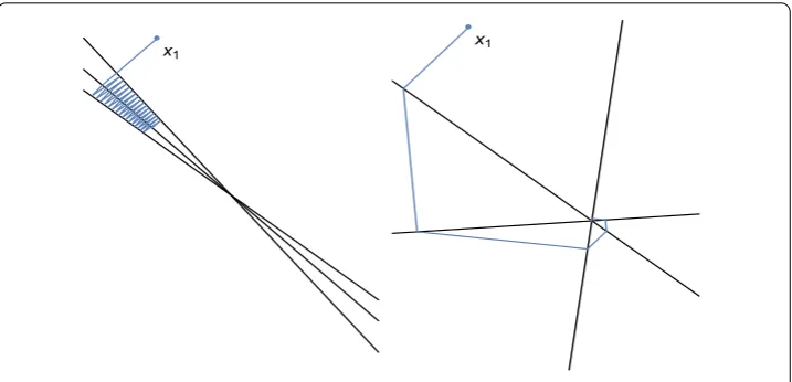
A new geometrical interpretation of the above can be described in the language of pro-jection methods. This conflicting behavior along singular vectors corresponds to projec-tions onto hyper-planes whose normal vectors are to a high degree identically aligned, i.e. for any two such normal vectorsn,n∈Rntheir dot product is close to unity. A toy
example forA∈R×that will be used for visualization is provided on the left in Figure . Such high degree of alignment poses challenges to classical projection methods since the progress made in each iteration is clearly humble. A much more favorable situation
applies when the normal vectors’ directions are spread close to evenly over the unit cir-cle so as to lower the conditioning of the problem. The system depicted on the right in Figure is obtained from the previous ill-conditioned one through the easily invertible Singular Value Homogenization (SVH) transformation (described below) and visibly fea-tures such better condition. Also plotted is the progress made by the classical Kaczmarz projection method which confirms the improved run-time (left: first iterations without convergence, right: convergence after seven steps).
3.1 The transformation
To achieve better condition numberκ(A) ofAwe directly manipulate its SVD through introducing the SVH matrix=diag(γ,γ, . . . ,γn)∈Rn×n(γi= ) to multiply the singular values (σ,σ, . . . ,σr), wherer≤min{n,m}is the rank ofA:
˜
A=UVT. (.)
By proper choice ofγ, . . . ,γr, the singular valuesσ˜, . . . ,σ˜r ofA˜ can be set to any arbi-trary values. In particular, they may be chosen suchκ(A˜) = . Consequently, solving the transformed problem
˜
Ax=z (.)
iteratively does not pose difficulties to most (projection) solvers. Assume (.) admits a solutionx˜, the question then is whether we can recover (easily) a solutionxsatisfying
Ax=z (.)
that is, the original linear subproblem.
Sinceleaves the range ofA,ranA⊂Rn, invariant, solutions to (.) exist if and only if (.) admits such. Moreover, setting
x=VVTx˜ (.)
a solution to (.) is obtained:
Ax=
UVTVVTx˜=
UVTx˜=A˜x˜=z. (.)
Thus by a scaling of the components ofx˜in the coordinate system ofA’s right singular
vectors, which computationally does not pose any difficulties, we can solve the original problem (.) by working out the solution to the simpler formulation (.).
Example . For geometric intuition, the assignment in (.) can be rewritten as
x=
V(–I) +IVTx˜
=x˜+
n
i=
˜
αi(γi– )·vi, (.)
Figure 2 Reconstruction ofx0(=xopt).
Equation (.) illustrates that the-transformation is in fact a translation of the solution set along these right singular vectors, proportional to the choice ofγi. The toy example from Figure is used to demonstrate this effect in Figure .
Here
A=
⎛ ⎜ ⎝
. .
⎞ ⎟
⎠, z=A·
, x=
(.)
with
σ= ., σ= ., κ(A) = . (.)
and right-singular vectors visualized in red.
Applying the-transformation withγ =σ and γ=σ/σ the transformed inverse
problemAx˜ =zis optimally conditioned withκ(A˜) = and hence easily solvable with so-lution
˜
x= (., .)T (.)
which is exactly the translation expected from (.).
3.2 Main result
The application of this preconditioning process to optimization problems with linear sub-problems as in (.) is the natural next step.
Theorem . Given a convex function f ∈C(Rn),then the minimization problem min
x∈Rmf(Ax) (.)
has solution
whereis a diagonal matrix with non-zero diagonal elements andx˜solves
min ˜
x∈Rmf(A˜˜x) (.)
withA as in˜ (.).
Proof For the minimizerxwe have
∇xf(Ax) =AT· ∇zf(z)|Ax= (.)
and hence
∇zf(z)|Ax∈ker
AT. (.)
The statement of the theorem is thus equivalent to showing
∇zf(z)|A˜x˜∈ker ˜
AT ⇒ ∇zf(z)|Ax∈ker
AT (.)
which follows from our previous observation that -transformations leave kernel and
range ofAinvariant together with (.).
3.3 The algorithmic scheme
The results of the previous two sections are straightforward to encode into a program usable for actual computation. What follows is a pseudo-code of the general scheme.
Algorithm .(Singular Value Homogenization)
Step : Letf andAbe given as in(.).
Step : Compute the SVD ofA=UVTand choose=diag(γ, . . . ,γm)such that
κA˜ =UVT≈. (.)
Step : Apply any optimization procedure to solve(.)and obtain a solutionx˜.
Step : Reconstruct the original solutionxof(.)via
x=VVTx˜. (.)
The optimal choices ofin Step and the concrete solver to findx˜in Step are likely
problem specific and are as of now left as user parameters. A parameter exploration to find all-purpose configurations is included in the next section.
Furthermore, due to the near-optimal conditioning in Step the time complexity of Al-gorithm . isO(min{mn,mn}) since it is dominated by the SVD ofA.
4 Numerical experiments
All testing was done in bothMatlabandMathematicawith negligible performance differences between the two (as both implement the same set of standard minimization algorithms).
4.1 Linear feasibility and linear least squares
The first series of experiments concerns the simplest and most often encountered formu-lation of (.) with
f(Ax) = Ax–b (.)
which corresponds to solving a linear system of equations exactly if a solution exist or in the least squares sense if it has empty intersection (hereb∈Rnis fixed).
As projection methods in general, and the Kaczmarz and Cimmino algorithms in par-ticular, are known to perform well in such settings, we chose to compare execution of Algorithm . to these two for benchmarking. Moreover, to isolate the effects of the -transformation most visibly, these two algorithms are used as subroutines in Step as well.
Performance was measured on a set{Ai∈R×}of , randomly generated matrices withκ(Ai)∈[, ] and datax= (, , )Tthat the respective algorithms were run on. The
convergence threshold in all cases was set to –andchosendsuch that=σ·I. The
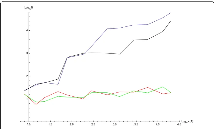
results are depicted in Figure and Figure (the presence of two graphs for Algorithm . indicate whether Kaczmarz (green) or Cimmino (red) was used as subroutine).
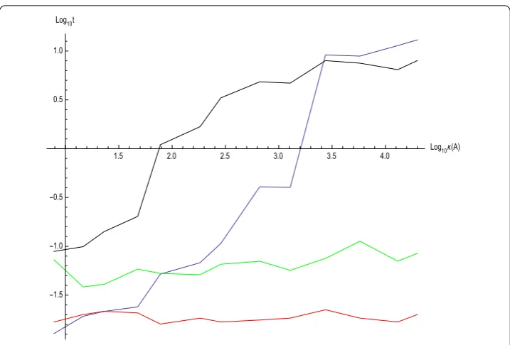
As expected from the results obtained in the preceding sections, both projection solvers scale poorly (indeed exponentially) with the condition number ofAwhile Algorithm . retains constant time (≈. s ande≈. s respectively) and numbers of iteration (≈) necessary.
Figure 3 Comparison with respect to number of iterations as a function of condition number between Kaczmarz, Cimmino and SVH with Kaczmarz and SVH with Cimmino.Stopping criteria is
Figure 4 Time needed: Algorithm 3.3 (red, green) and Kaczmarz (blue) and Cimmino (black) methods.
In addition, reducing the accuracy threshold (< –) or constructing matrices of
ex-treme condition (κ(A)≥) that result in failure to converge of Cimmino, Kaczmarz and
LAPACK solvers native to Matlab and Mathematica does not impair the performance of Algorithm .. That is, through appropriate-transformation we were able to solve very ill-conditioned linear problems for the first time to –accuracy within seconds.
4.2 Lppenalties and one-sidedLppenalties
In the biomedical field of cancer treatment planning problems of the kind (.) occur often in calculating the optimal dose deposition in patient tissue. A typical formulation involves the linearized convolutionAof radiationxinto dosedand a reference doser∈Rnwhich is to be achieved underLppenalties Ax–r por their one-sided variations max{,Ax–r} p and min{,Ax–r} p.
We examined fivefcases{Ai,ri}that were collected from patient data under the penalties
f(d) = d–r , (.)
f(d) = d–r , (.)
f(d) =max(,d–r), (.)
f(d) =min(,d–r), (.)
f(d) =f(d·s) +f(d·s) +f(d·s) +f(d·s), (.)
wheresi∈ {, }nwith
si=1Rn is a partition of the unit vector accounting for varied sensitivity of distinct body tissue to radiation.
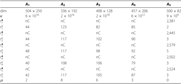
Table 1 Comparison for nonlinear objective function
A1 A2 A3 A4 A5
dim 504×250 336×192 408×128 457×206 500×82
κ 6×10¹⁶ 2×10¹⁶ 2×10¹⁸ 6×10¹² 9×10⁹
t•1 nC nC nC nC 2,381
t◦1 44 123 82 85 2
t•2 nC nC nC nC 2,445
t◦2 44 117 102 90 3
t•3 nC nC nC nC 2,579
t◦3 48 117 98 92 5
t•4 nC nC nC nC 2,502
t◦4 40 108 106 79 3
t•5 nC nC nC nC 2,524
t◦5 42 117 105 87 3
μ 2 8 6 3 0
needed for Algorithm . to converge. In the case of neither Mathematica nor Matlab find-ing a solution (nCfornot converging), the accuracy of Algorithm .’s outputxis tested
through the parameterμ. This is done by randomly sampling a neighborhood ofxand
counting instances that improve the objective. These hits are then sampled similarly until no further such points can detected.μis the total number of neighborhoods so checked. In all cases, the improvement inf remained below –.
The results are parallel to what could be seen in the linear feasibility formulation and encourage further exploration.
5 Conclusion
We were able to reduce the time needed to solve a general convex optimization problem with linear subproblem for modestly sized matrices. The performance of the proposed algorithm was compared to classical LAPACK and projection methods which showed an improvement in run-times by a factor of up to ,. Additionally, in many cases where LAPACK and projection solvers failed to converge, the singular value homogenization found –accurate solutions. These results are promising and encourage further
explo-ration of SVH. Especially its application to structured large matrices and constrained op-timization as well as in-depth parameter explorations may well turn out to be worthwhile.
Competing interests
The authors declare that they have no competing interests.
Authors’ contributions
D.-D. Erdmann-Pham, A. Gibali and P. Süss contributed equally to the writing of this paper. K.-H. Küfer, the head of the Optimization Department in Fraunhofer - ITWM provide technical and general support. All authors read and approved the final manuscript.
Author details
1Mathematics Department, Jacobs University, Bremen, 28759, Germany.2Mathematics Department, ORT Braude College,
Karmiel, 21982, Israel. 3Optimization Department, Fraunhofer - ITWM, Kaiserslautern, 67663, Germany.
Acknowledgements
This work was supported by the Fraunhofer Institute for Industrial Mathematics - ITWM.
Endnotes
a We choseRonly as it is more pertinent to most practical applications, the extension of all results toCis
straightforward.
b Which is particularly important in intensity modulated radiation therapy IMRT from which later numerical
c Majorandminorhere refer to the size of the singular values associated with a singular vector.
d Experimental evidence suggests that in this setting of randomized matrices such homogenization to one singular
value represents the most reasonable choice; differentdisplay similar behavior with overall longer run-times.
e This time difference is due to the higher overhead required for the block projections of the Cimmino algorithm. f The dose calculations are of cancerous tissue in the brain, the neck region and the prostate.
Received: 19 September 2015 Accepted: 7 January 2016
References
1. Sadek RA. SVD based image processing applications: state of the art, contributions and research challenges. Int J Adv Comput Sci Appl. 2012;3:26-34.
2. Rajwade A, Rangarajan A, Banerjee A. Image denoising using the higher order singular value decomposition. IEEE Trans Pattern Anal Mach Intell. 2013;35:849-61.
3. Levitin ES, Polyak BT. Constrained minimization problems. USSR Comput Math Math Phys. 1966;6:1-50. 4. Golshtein EG, Tretyakov NV. Modified Lagrangians and monotone maps in optimization. New York: Wiley; 1996. 5. Erhel J, Guyomarc’h F, Saad Y. Least-squares polynomial filters for ill-conditioned linear system. Thème 4 - Simulation
et optimisation de systèmes complexes. Projet ALADIN, Rapport de recherche N◦4175, Mai 2001, 28 pp.
6. Meng X, Saunders MA, Mahoney MW. LSRN: a parallel iterative solver for strongly over- or underdetermined systems. SIAM J Sci Comput. 2014;36:95-118.
7. Engl HW, Hanke M, Neubauer A. Regularization of inverse problems. Dordrecht: Kluwer Academic; 1996. 8. Vogel CR. Computational methods for inverse problems. Philadelphia: Society for Industrial and Applied
Mathematics; 2002.
9. Orkisz J, Pazdanowski M. On a new feasible directions solution approach in constrained optimization. In: Onate E, Periaux J, Samuelsson A, editors. The finite element method in the 1990’s. Berlin: Springer; 1991. p. 621-32. 10. Pazdanowski M. SVD as a preconditioner in nonlinear optimization. Comput Assist Mech Eng Sci. 2014;21:141-50. 11. Goebel K, Reich S. Uniform convexity, hyperbolic geometry, and nonexpansive mappings. New York: Marcel Dekker;
1984.
12. Censor Y, Zenios SA. Parallel optimization: theory, algorithms, and applications. New York: Oxford University Press; 1997.
13. Galántai A. Projectors and projection methods. Dordrecht: Kluwer Academic; 2004.
14. Escalante R, Raydan M. Alternating projection methods. Philadelphia: Society for Industrial and Applied Mathematics; 2011.
15. Bauschke HH, Combettes PL. Convex analysis and monotone operator theory in Hilbert spaces. Berlin: Springer; 2011. 16. Censor Y, Chen W, Combettes PL, Davidi R, Herman GT. On the effectiveness of projection methods for convex
feasibility problems with linear inequality constraints. Comput Optim Appl. 2012;51:1065-88.
17. Bauschke HH, Koch VR. Projection methods: Swiss Army knives for solving feasibility and best approximation problems with halfspaces. Contemp Math. 2015;636:1-40.