R E S E A R C H
Open Access
A primal-dual fixed point algorithm for
minimization of the sum of three convex
separable functions
Peijun Chen
1,2,3, Jianguo Huang
1and Xiaoqun Zhang
1,4**Correspondence:
1Schools of Mathematical Sciences,
and MOE-LSC, Shanghai Jiao Tong University, 800, Dongchuan Road, Shanghai, China
4Institute of Natural Sciences,
Shanghai Jiao Tong University, 800, Dongchuan Road, Shanghai, China Full list of author information is available at the end of the article
Abstract
Many problems arising in image processing and signal recovery with
multi-regularization and constraints can be formulated as minimization of a sum of three convex separable functions. Typically, the objective function involves a smooth function with Lipschitz continuous gradient, a linear composite nonsmooth function, and a nonsmooth function. In this paper, we propose a primal-dual fixed point (PDFP) scheme to solve the above class of problems. The proposed algorithm for three-block problems is a symmetric and fully splitting scheme, only involving an explicit
gradient, a linear transform, and the proximity operators which may have a closed-form solution. We study the convergence of the proposed algorithm and illustrate its efficiency through examples on fused LASSO and image restoration with non-negative constraint and sparse regularization.
Keywords: primal-dual fixed point algorithm; convex separable minimization; proximity operator; sparsity regularization
1 Introduction
In this paper, we aim to design a primal-dual fixed point algorithmic framework for solving the following minimization problem:
min
x∈Rnf(x) + (f◦B)(x) +f(x), (.) wheref,f, andfare three proper lower semi-continuous convex functions, andfis dif-ferentiable onRnwith a /β-Lipschitz continuous gradient for someβ∈(, +∞], while
B:Rn→Rmis a linear transformation. This formulation covers a wide application in im-age processing and signal recovery with multi-regularization terms and constraints. For instance, in many imaging and data processing applications, the functionalfcorresponds to a data-fidelity term, and the last two terms are used for regularization. As a direct ex-ample of (.), we can consider the fused LASSO penalized problem [, ] defined by
min x∈Rn
Ax–a +μ
Bx+μx.
On the other hand, in the imaging science, total variation regularization withBbeing the discrete gradient operator together withregularization has been adopted in some
image restoration applications, for example in []. Another useful application corresponds tof=χC, whereχCis the indicator function of a nonempty closed convex setC. In this case, the problem reduces to
min
x∈Cf(x) + (f◦B)(x). (.)
As far as we know, Combettes and Pesquet first proposed a fully splitting algorithm in [] to solve monotone operator inclusions problems, which include (.) as a special case. Condat [] tackled the same problem and proposed a primal-dual splitting scheme. Exten-sions to multi-block composite functions are also discussed in detail. For the special case
B=I(Idenotes the usual identity operator), Davis and Yin [] proposed a three-operator splitting scheme based on monotone operators. For the case that the problem (.) re-duces to two-block separable functions, many splitting and proximal algorithms have been proposed and studied in the literature. Among them, extensive research have been con-ducted on the alternating direction of multiplier method (ADMM) [] (also known as split Bregman []; see for example [] and the references therein). The primal-dual hybrid gradient method (PDHG) [–], also known as the Chambolle-Pock algorithm [], is another class of popular algorithm, largely adopted in imaging applications. In [–], several completely decoupled schemes, such as the inexact Uzawa solver and primal-dual fixed point algorithm, are proposed to avoid subproblem solving for some typical min-imization problems. Komodakis and Pesquet [] recently gave a nice overview of recent primal-dual approaches for solving large-scale optimization problems (.). A general class of multi-step fixed point proximity algorithms is proposed in [], which covers several ex-isting algorithms [, ] as special cases. In the preparation of this paper, we notice that Li and Zhang [] also studied the problem (.) and introduced a quasi-Newton and the overrelaxation strategies for accelerating the algorithms. Both algorithms can be viewed as a generalization of Condat’s algorithm []. The theoretical analysis is established based on the multi-step techniques present in [].
In the following, we mainly review some most relevant work for a concise presentation. Problem (.) has been studied in [] in the context of maximum a posterior ECT recon-struction, and a preconditioned alternating projection algorithm (PAPA) is proposed for solving the resulting regularization problem. Forf= in (.), we proposed the primal-dual fixed point algorithm PDFPO (primal-dual fixed point algorithm based on proximity operator) in []. Based on the fixed point theory, we have shown the convergence of the scheme PDFPO and the convergence rate of the iteration sequence under suitable con-ditions.
In this work, we aim to extend the ideas of the PDFPO in [] and the PAPA in [] for solving (.) without subproblem solving and provide a convergence analysis on the primal-dual sequences. The specific algorithm, namely the primal-dual fixed point (PDFP) algorithm, is formulated as follows:
(PDFP)
⎧ ⎪ ⎪ ⎨ ⎪ ⎪ ⎩
yk+=proxγf(xk–γ∇f(xk) –λBTvk),
vk+= (I–proxγ
λf)(By
k++vk),
xk+=proxγf(xk–γ∇f(xk) –λBTvk+),
where <λ< /λmax(BBT), <γ < β. Hereprox
fis the proximity operator [] of a func-tionf; see (.). Whenf=χC, the proposed algorithm (.) is reduced to the PAPA pro-posed in []; see (.). For another special case,f= in (.), we obtain the PDFPO proposed in []; see (.). The convergence analysis of this PDFP algorithm is built upon fixed point theory on the primal and dual pairs. The overall scheme is completely ex-plicit, which allows for an easy implementation and parallel computing for many large-scale applications. This will be further illustrated through application to the problems arising in statistics learning and image restoration. The PDFP has a symmetric form and it is different from Condat’s algorithm []. In addition, we point out that the ranges of the parameters in PDFP are larger than those of [, ] and the rules for the parame-ters in PDFP are well separated, which could be advantageous in practice compared to [, ].
The rest of the paper is organized as follows. In Section , we will present some pre-liminaries and notations, and deduce PDFP from the first order optimality condition. In Section , we will provide the convergence results and the linear convergence rate results for some special cases. In Section , we will make a comparison on the form of the PDFP algorithm (.) with some existing algorithms. In Section , we will show the numerical performance and the efficiency of PDFP through some examples on fused LASSO and pMRI (parallel magnetic resonance image) reconstruction.
2 Primal-dual fixed point algorithm 2.1 Preliminaries and notations
For the self completeness of this work, we list some relevant notations, definitions, as-sumption and lemmas in convex analysis. We refer the reader to [, ] and the references therein for more details.
For the ease of presentation, we restrict our discussion to Euclidean spaceRn, equipped with the usual inner product·,· and norm·=·,· /. We first assume that the problem (.) has at least one solution andf,f,Bsatisfy
∈ridomf–B(domf)
, (.)
where the symbolri(·) denotes the interior of a convex subset, and the effective domain of
f is defined asdomf={x∈Rn|f(x) < +∞}.
Thenorm of a vectorx∈Rnis denoted by · and the spectral norm of a matrix is denoted by · . Let(Rn) be the collection of all proper lower semi-continuous convex functions fromRnto (–∞, +∞]. For a functionf ∈(Rn), the proximity operator off: proxf [] is defined by
proxf(x) =arg min y∈Rn f
(y) + x–y
. (.)
For a nonempty closed convex setC⊂Rn, letχ
Cbe the indicator function ofC, defined by
χC(x) =
⎧ ⎨ ⎩
LetprojCbe the projection operator ontoC,i.e.
projC(x) =arg min y∈C
x–y.
It is easy to see thatproxγ χ
C=projCfor allγ > , and the proximity operator is a gener-alization of projection operator. Note that many efficient splitting algorithms rely on the fact thatproxfhas a closed-form solution. For example, whenf =γ · , the proximity so-lution is given by element-wise soft-shrinking. We refer the reader to [] for more details as regards proximity operators. Let∂f be the subdifferential off,i.e.
∂f(x) =v∈Rn| y–x,v ≤f(y) –f(x) for ally∈Rn , (.) andf∗be the convex conjugate function off, defined by
f∗(x) =sup
y∈Rnx,y –f(y).
An operatorT:Rn→Rnis nonexpansive if Tx–Ty ≤ x–y for allx,y∈Rn,
andTis firmly nonexpansive if
Tx–Ty≤ Tx–Ty,x–y for allx,y∈Rn.
It is obvious that a firmly nonexpansive operator is nonexpansive. An operator T is δ-strongly monotone if there exists a positive real numberδsuch that
Tx–Ty,x–y ≥δx–y for allx,y∈Rn. (.)
Lemma . For any two functions f∈(Rm)and f∈(Rn),and a linear
transforma-tion B:Rn→Rm,satisfying that∈ri(dom
f–B(domf)),we have
∂(f◦B+f) =BT◦∂f◦B+∂f.
Lemma . Let f∈(Rn).Thenproxfand I–proxf are firmly nonexpansive.In addition,
x=proxf(y) ⇔ y–x∈∂f(x) for a given y∈Rn, (.)
y∈∂f(x) ⇔ x=proxf(x+y)
⇔ y= (I–proxf)(x+y) for x,y∈Rn, (.)
x=proxγf(x) +γprox γf∗
γx
for all x∈Rnandγ> . (.)
If f has/β-Lipschitz continuous gradient further,we have
Lemma . Let T be an operator and u∗be a fixed point of T.Let{uk+}be the sequence
generated by the fixed point iteration uk+=T(uk).Suppose(i)T is continuous, (ii){uk–
u∗}is non-increasing, (iii)limk→+∞uk+–uk= .Then the sequence{uk}is bounded
and converges to a fixed point of T.
The proof of Lemma . is standard, and we refer the reader to the proof of Theorem . in [] for more details.
Letγ andλbe two positive numbers. To simplify the presentation, we use the following notations:
T(v,x) =proxγf
x–γ∇f(x) –λBTv, (.)
T(v,x) = (I–proxγ λf)
B◦T(v,x) +v, (.)
T(v,x) =proxγfx–γ∇f(x) –λBT◦T(v,x), (.)
T(v,x) =T(v,x),T(v,x). (.) Denote
g(x) =x–γ∇f(x) for allx∈Rn, (.)
M=I–λBBT. (.)
Letλmax(A) denote the largest eigenvalue of a square matrixA. When <λ< /λmax(BBT),
Mis a symmetric and positive definite matrix, so we can define a norm vM=
v,Mv for allv∈Rm. (.)
For a pairu= (v,x)∈Rm×Rn, we also define a norm on the product spaceRm×Rnas uλ=
λv+x. (.)
2.2 Derivation of PDFP
On extending the ideas of the PAPA proposed in [] and the PDFPO proposed in [], we derive the primal-dual fixed point algorithm (.) for solving the minimization problem (.).
Under the assumption (.), by using the first order optimality condition of (.) and Lemma ., we have
∈γ∇f
x∗+λBT∂
γ λf
Bx∗+γ ∂f
x∗,
wherex∗is an optimal solution. Let
v∗∈∂
γ λf
Bx∗. (.)
By applying (.), we have
v∗= (I–proxγ λf)
x∗=proxγf
x∗–γ∇f
x∗–λBTv∗. (.)
By inserting (.) into (.), we get
v∗= (I–proxγ λf)
B◦proxγfx∗–γ∇f
x∗–λBTv∗+v∗,
or equivalently,v∗=T(v∗,x∗). Next, replacingv∗ in (.) byT(v∗,x∗), we can getx∗=
T(v∗,x∗). In other wordsu∗=T(u∗) foru∗= (v∗,x∗). Meanwhile, ifu∗=T(u∗), we can see thatx∗ meets the first order optimality condition of (.) and thusx∗ is a minimizer of (.).
To sum up, we have the following theorem.
Theorem . Suppose that x∗is a solution of (.)and v∗∈Rmis defined as(.).Then
we have
⎧ ⎨ ⎩
v∗=T(v∗,x∗),
x∗=T(v∗,x∗),
i.e. u∗= (v∗,x∗)is a fixed point of T.Conversely,if u∗= (v∗,x∗)∈Rm×Rnis a fixed point
of T,then x∗is a solution of (.).
It is easy to confirm that the sequence{(vk+,xk+)}generated by the PDFP algorithm (.) is the Picard iteration (vk+,xk+) =T(vk,xk). So we will use the operatorTto analyze the convergence of the PDFP in Section .
3 Convergence analysis
In the following, let{yk+}and{uk+= (vk+,xk+)}be the sequences generated by the PDFP algorithm (.),i.e. yk+=T
(vk,xk) and (vk+,xk+) =T(vk,xk). Letu∗= (v∗,x∗) be a fixed point of the operatorT.
3.1 Convergence
Lemma . We have the following estimates:
vk+–v∗≤vk–v∗–vk+–vk+ BTvk+–v∗,yk+–x∗, (.)
xk+–x∗≤xk–x∗–xk+–yk+–xk–yk+
+ xk+–yk+,γ∇f
xk+λBTvk
– xk+–x∗,γ∇f
xk+λBTvk++ γf
x∗–f
yk+. (.)
Proof We first prove (.). By Lemma ., we knowI–proxγ
λfis firmly nonexpansive, and
using (.)and (.) we further have
vk+–v∗≤vk+–v∗,Byk++vk–Bx∗+v∗,
which implies
Thus
vk+–v∗ =vk–v∗–vk+–vk+ vk+–v∗,vk+–vk
≤vk–v∗–vk+–vk+ BTvk+–v∗,yk+–x∗.
Next we prove (.). By the optimality condition of (.)(cf.(.)), we have
xk–γ∇f
xk–λBTvk+–xk+∈γ ∂f
xk+.
By the property of subdifferentials (cf.(.)),
x∗–xk+,xk–γ∇f
xk–λBTvk+–xk+≤γf
x∗–f
xk+,
i.e.
xk+–x∗,xk+–xk≤–xk+–x∗,γ∇f
xk+λBTvk++γf
x∗–f
xk+.
Therefore,
xk+–x∗ =xk–x∗–xk+–xk+ xk+–x∗,xk+–xk
≤xk–x∗–xk+–xk– xk+–x∗,γ∇f
xk+λBTvk+
+ γf
x∗–f
xk+. (.)
On the other hand, by the optimality condition of (.), it follows that
xk–γ∇f
xk–λBTvk–yk+∈γ ∂f
yk+.
Thanks to the property of subdifferentials, we have
xk+–yk+,xk–γ∇f
xk–λBTvk–yk+≤γf
xk+–f
yk+.
So
xk+–yk+,xk–yk+≤xk+–yk+,γ∇f
xk+λBTvk+γf
xk+–f
yk+.
Thus
–xk+–xk = –xk+–yk+–xk–yk++ xk+–yk+,xk–yk+
≤–xk+–yk+–xk–yk++ xk+–yk+,γ∇f
xk+λBTvk
+ γf
xk+–f
yk+.
Replacing the term –xk+–xkin (.) with the right side term of the above inequality,
Lemma . We have
uk+–u∗
λ≤u
k–u∗
λ–λv
k+–vk M–x
k+–yk++λBTvk+–vk –xk–yk+–γ∇f
xk–γ∇f
x∗
–γ(β–γ)∇f
xk–∇f
x∗. (.)
Proof Summing the two inequalities (.) and (.) and re-arranging the terms, we have λvk+–v∗+xk+–x∗
≤λvk–v∗+xk–x∗–λvk+–vk–xk+–yk+–xk–yk+
+ λBTvk+–v∗,yk+–x∗+ xk+–yk+,γ∇f
xk+λBTvk
– xk+–x∗,γ∇f
xk+λBTvk++ γf
x∗–f
yk+
=λvk–v∗+xk–x∗–λvk+–vk–xk+–yk+–xk–yk+
+ λBTvk+–vk,yk+–xk++ xk–yk+,γ∇f
xk–γ∇f
x∗
– xk–x∗,γ∇f
xk–γ∇f
x∗
+ yk+–x∗, –γ∇f
x∗–λBTv∗+γf
x∗–f
yk+
=λvk–v∗+xk–x∗–λvk+–vkM–xk+–yk++λBTvk+–vk
–xk–yk+–γ∇f
xk–γ∇f
x∗+γ∇f
xk–γ∇f
x∗
– xk–x∗,γ∇f
xk–γ∇f
x∗
+ yk+–x∗, –γ∇f
x∗–λBTv∗+γf
x∗–f
yk+, (.)
where · Mis given in (.) and (.). Meanwhile, by the optimality condition of (.), we have
–γ∇f
x∗–λBTv∗∈γ ∂f
x∗, which implies
yk+–x∗, –γ∇f
x∗–λBTv∗+γf
x∗–f
yk+≤. (.)
On the other hand, it follows from (.) that
–xk–x∗,∇f
xk–∇f
x∗≤–β∇f
xk–∇f
x∗. (.)
Recalling (.), we immediately obtain (.) in terms of (.)-(.).
Lemma . Let <λ< /λmax(BBT)and <γ < β.Then the sequence{uk–u∗
λ}is
non-increasing andlimk→+∞uk+–ukλ= .
Proof If <λ< /λmax(BBT) and <γ< β, it follows from (.) thatuk+–u∗λ≤ uk–
(.) fromk= tok= +∞, we get lim
k→+∞
vk+–vkM= , (.)
lim k→+∞x
k+–yk++λBTvk+–vk= , (.) lim
k→+∞x
k–yk+–γ∇f
xk–γ∇f
x∗= , (.)
lim k→+∞∇f
xk–∇f
x∗= . (.)
The combination of (.) and (.) gives
lim k→+∞x
k–yk+= . (.)
Noting that <λ< /λmax(BBT), we knowMis symmetric and positive definite, so (.) is equivalent to
lim k→+∞v
k+–vk= . (.)
Hence, we have from the above inequality and (.) that
lim k→+∞
xk+–yk+= . (.)
The combination of (.) and (.) then gives rise to
lim k→+∞
xk+–xk= . (.)
According to (.), (.), and (.), we havelimk→+∞uk+–uk
λ= .
As a direct consequence of Lemma . and Lemma ., we obtain the convergence of the PDFP as follows.
Theorem . Let <λ< /λmax(BBT)and <γ< β.Then the sequence{uk}is bounded
and converges to a fixed point of T,and both{xk}and{yk}converge to a solution of (.).
Proof By Lemma ., bothproxγf
andI–proxγλfare firmly nonexpansive, thus the
oper-atorTdefined by (.)-(.) is continuous. From Lemma ., we know that the sequence {uk–u∗λ}is non-increasing and limk→+∞uk+–ukλ= . By using Lemma ., we
know that the sequence{uk}is bounded and converges to a fixed point of T. By using Theorem . and (.), we can conclude that both{xk}and{yk}converge to a solution
of (.).
Remark . For the special casef= , the PDFP reduces naturally to the PDFPO (.) proposed in [], where the conditions for the parameters are <λ≤/λmax(BBT), < γ < β. In the proof of Lemma ., we utilize the positive definitiveness ofMto obtain (.) from (.). So the condition for the parameterλis slightly more restricted as < λ< /λmax(BBT) in Lemma . and Theorem .. Whenf
of Lemma . can also be relaxed to <λ≤/λmax(BBT). As a matter of fact, it is easy to check by the definition ofyk+(see (.)) and the optimality condition of (.) that
xk–yk+–γ∇f
xk–γ∇f
x∗=λBTvk–v∗. (.) Observing thatvk+–vk=vk+–vk
M+λBT(vk+–vk), we have by (.), (.) and (.) thatlimk→+∞vk+–vk= . Therefore we can derive the convergence wheneverM is semi-positive definite forf= .
Remark . For the special casef= , the problem (.) only corresponds to two proper lower semi-continuous convex functions. The convergence condition <γ < β in the PDFP becomes <γ < +∞. Althoughγ is an arbitrary positive number in theory, the range ofγ will affect the convergence speed and it is also a difficult problem to choose a best value in practice.
3.2 Linear convergence rate for special cases
In the following, we will show the convergence rate results with some additional as-sumptions on the basic problem (.). In particular, forf= , the algorithm reduces to the PDFPO proposed in []. The conditions for a linear convergence given there as Condition . in [] is as follows: for <λ≤/λmax(BBT) and <γ < β, there exist η,η∈[, ) such that
I–λBBT≤η,
g(x) –g(y)≤ηx–y for allx,y∈Rn, (.)
whereg(x) is given in (.). It is easy to see that a strongly convex functionfsatisfies the condition (.). For a generalf, we need stronger conditions on the functions.
Theorem . Suppose that(.)holds and f∗is strongly convex.Then we have
uk+–u∗(+λδ/γ)λ≤ηuk–u∗(+λδ/γ)λ,
where <η< is the convergence rate(indicated in the proof)andδ> is a parameter describing the strongly monotone property of∂f∗(cf.(.)).
Proof Use Moreau’s identity (cf.(.)) to get
(I–proxγ λf)
Byk++vk=γ
λproxγλf∗
λ γBy
k++λ γv
k
.
So (.)is equivalent to
λ γv
k+=prox
λ γf∗
λ γBy
k++λ γv
k
. (.)
According to the optimality condition of (.),
λ γBy
k++λ γv
k– λ γv
k+∈ λ γ∂f
∗
λ γv
k+
Similarly, according to the optimality condition of (.),
λ γBx
∗∈ λ
γ∂f
∗
λ γv
∗. (.)
Observing that∂f∗isδ-strongly monotone, we have by (.) and (.)
vk+–v∗,Byk++vk–vk+–Bx∗≥ λ
γδv
k+–v∗,
i.e.
vk+–v∗,vk+–vk≤BTvk+–v∗,yk+–x∗– λ γδv
k+–v∗ .
Thus
vk+–v∗ =vk–v∗–vk+–vk+ vk+–v∗,vk+–vk
≤vk–v∗–vk+–vk+ BTvk+–v∗,yk+–x∗ –λ
γδv
k+–v∗
. (.)
Summing the two inequalities (.) and (.), and then using the same argument for driving (.), we arrive at
+λ γδ
λvk+–v∗+xk+–x∗≤λvk–v∗+gxk–gx∗
≤λvk–v∗+ηxk–x∗, (.)
where we have also used the condition (.) and the inequality (.).
Letη= /√ +λδ/γ andη=max{η,η}. It is clear that <η< . Hence, according to the notation (.), the estimate (.) can be rewritten as required.
We note that a linear convergence rate for strongly convex f∗ andf are obtained in []. They introduced two preconditioned operators for accelerating the algorithm, while a clear relation between the convergence rate and the preconditioned operators is still missing. Meanwhile, introducing preconditioned operators could be beneficial in practice, and we can also introduce a preconditioned operator to deal with∇fin our scheme. Since the analysis is rather similar to the current one, we will omit it in this paper.
4 Connections to other algorithms
In this section, we present the connections of the PDFP algorithm to some algorithms proposed previously in the literature.
In particular, whenf=χC, due toproxγf =projC, the proposed algorithm (.) is
re-duced to the PAPA proposed in []
(PDFP)
⎧ ⎪ ⎪ ⎨ ⎪ ⎪ ⎩
yk+=projC(xk–γ∇f(xk) –λBTvk),
vk+= (I–proxγ
λf)(By
k++vk),
xk+=projC(xk–γ∇f(xk) –λBTvk+),
where <λ< /λmax(BBT), <γ < β. We note that the conditions of the parameters for the convergence of the PDFP are larger than those in []. Here we still refer to (.) as the PDFP, since the PAPA originally proposed in [] incorporates other techniques such as diagonal preconditioning.
For the special casef= , due toproxγf=I, we obtain the PDFP
O scheme proposed in []
PDFPO
⎧ ⎪ ⎪ ⎨ ⎪ ⎪ ⎩
yk+=xk–γ∇f(xk) –λBTvk,
vk+= (I–proxγ
λf)(By
k++vk),
xk+=xk–γ∇f
(xk) –λBTvk+,
(.)
where <λ≤/λmax(BBT), <γ < β. Recently, we notice that the PDFPO reduces to the algorithm previously proposed forf(x) =Ax–aby Loris and Verhoeven in []. The convergence and the convergence rate of the objective function were established in [], but the convergence conditions are slightly more restrictive than the ones given in []. On the other hand, we emphasize that the PDFPO algorithm can also be interpreted from the point of view of forward-backward operator splitting, as shown in [, ]. More-over, the multi-block formulation was devised and analyzed in [].
Based on the PDFPO, we also proposed the PDFPOCin [] forf=χCas
PDFPOC
⎧ ⎪ ⎪ ⎪ ⎪ ⎪ ⎨ ⎪ ⎪ ⎪ ⎪ ⎪ ⎩
yk+=xk–γ∇f(xk) –λBTvk–λvk,
vk+= (I–proxγ λf)(By
k++vk ),
vk+
= (I–projC)(yk++vk),
xk+=xk–γ∇f(xk) –λBTvk+ –λvk+,
(.)
where <λ≤/(λmax(BBT) + ), <γ < β. A similar technique of extension to multi-composite functions has also been used in [, , ]. Compared to the PDFP (.), the algorithm PDFPOCintroduces an extra variable, while the PDFP requires two times pro-jections. Most importantly, the primal variable at each iterate of the PDFP is feasible, but maybe not for that of the PDFPOC. In addition, the permitted ranges of the parameters are also tighter in the PDFPOC.
Another interesting special case isf= . The scheme (.) reduces to
(PDFP) ⎧ ⎪ ⎪ ⎨ ⎪ ⎪ ⎩
yk+=prox
γf(x
k–λBTvk),
vk+= (I–proxγ
λf)(By
k++vk),
xk+=prox
γf(x
k–λBTvk+),
(.)
where <λ< /λmax(BBT), <γ < +∞. It is easy to see that (.) is different from the PDHG method in [, ] and (.) has a symmetric step (.)compared to the extrapo-lation step in the PDHG method.
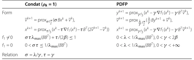
Table 1 The comparison between Condat (ρk= 1) and PDFP
Condat (ρk= 1) PDFP
Form
vk+1= proxσf2∗(σBxk+vk), xk+1= prox
τf3(xk–τ∇f1(xk) –τBT(2vk+1–vk))
yk+1= prox
γf3(xk–γ∇f1(xk) –γBTvk), vk+1= proxλ
γf2∗(
λ γByk+1+v
k),
xk+1= proxγf3(x
k–γ∇f
1(xk) –γBTvk+1)
f1= 0 σ τ λmax(BBT) +τ/(2β)≤1 0 <λ< 1/λmax(BBT), 0 <γ< 2β
f1= 0 0 <σ τ≤1/λmax(BBT) 0 <λ< 1/λmax(BBT), 0 <γ< +∞
Relation σ=λ/γ,τ=γ
as studied in []. Condat [] tackled the same problem as given in (.) and proposed a primal-dual splitting scheme. For the special case withf= , Condat’s algorithm reduces to the PDHG method in []. By grouping the multi-block as two blocks, the authors in [] extended the PDHG algorithm [] to the minimization of sum of multi-composite func-tions. The authors in [] proposed a class of multi-step fixed point proximity algorithms, including several existing algorithms as special examples, for example the algorithms in [, ]. In [], Davis and Yin proposed a operator splitting method for solving three-block monotone inclusions in a very tricky way. When solving the problem (.) withB=I, the scheme is different from Condat’s algorithm and PDFP algorithm. But it requires sub-problem solving ifB=I. Li and Zhang [] studied (.) based on the techniques present in [] and including Condat’s algorithm in [] as a special case, and further introduced quasi-Newton and the overrelaxation strategies to accelerate the algorithms.
In the following, we mainly compare PDFP to the basic Algorithm . proposed by Condat in [] to simplify the presentation. We first change the form of the PDFP algo-rithm (.) by using Moreau’s identity, see (.),i.e.
(I–proxγ λf)
Byk++vk=γ
λproxγλf∗
λ γBy
k++vk
,
wherevk=γλvk. A direct comparison is presented in Table . From Table , we can see that the ranges of the parameters in Condat’s algorithm are relatively smaller than PDFP. Also since the condition for Condat’s algorithm is mixed with all the parameters, it is not always easy to choose them in practice. This is also pointed out in []. While the rules for the parameters in PDFP are separate, and they can be chosen independently accord-ing to the Lipschitz constant and the operator norm ofBBT. In this sense, our parame-ter rules are relatively more practical. In the numerical experiments, we can setλto be close to /λmax(BBT) andγ to be close to β for most of tests. Moreover, the results of
xk–γ∇f(xk) andλBTvk+can be stored as two intermediate variables that can be reused in (.)and (.)during the iterations. Nevertheless, PDFP has an extra step (.) com-pared to Condat’s algorithm and the computation cost may increase due to the compu-tation ofproxγf. In practice, this step is often related to the shrinkage or projection operation being easy to implement, so the cost could be still ignorable in practice.
5 Numerical experiments
5.1 The fused LASSO penalized problem
The fused LASSO (least absolute shrinkage and selection operator) penalized problem is proposed for group variable selection, and we refer the reader to [, , ] for more details for the applications of this model. It can be described as
min x∈Rn
Ax–a +μ
n–
i=
|xi+–xi|+μx.
HereA∈Rr×n,a∈Rr. The row ofA:A
ifori= , , . . . ,rrepresent theith observation of the independent variables andaidenotes the response variable, and the vectorx∈Rnis the regression coefficient to recover. The first term is corresponding to the data-fidelity term, and the last two terms aim to ensure the sparsity in both xand their successive differences inx. Let
B=
⎛ ⎜ ⎜ ⎜ ⎜ ⎝
– –
. .. ... –
⎞ ⎟ ⎟ ⎟ ⎟ ⎠.
Then the forgoing problem can be reformulated as
min x∈Rn
Ax–a +μ
Bx+μx. (.)
For this example, we can setf(x) =Ax–a,f
=μ · ,f=μ · . We want to show that the PDFP algorithm (.) can be applied to solve this generic class of problems (.) directly and easily.
The following tests are designed for the simulation. We setr= ,n= ,, and the dataais generated asAx+αe, whereAandeare random matrices whose elements are normally distributed with zero mean and variance , andα= ., andxis a generated sparse vector, whose nonzero elements are showed in Figure by green ‘+’. We setμ= , μ= , and the maximum iteration number asItn= ,.
We compare the PDFP algorithm with Condat’s algorithm []. For the PDFP algo-rithm, the parametersλandγ are chosen according to Theorem .. In practice, we set λto be close to /λmax(BBT) and γ to be close to β. Here we setλ= / as then– eigenvalues ofBBTcan be analytically computed as – cos(iπ/n),i= , , . . . ,n– and γ = ./λmax(ATA). For Condat’s algorithm, we setλ= ./,γ = ./λmax(ATA), which is chosen for a relative better numerical performance. The computation time, the attained objective function values, and the relative errors to the true solution are close for Condat’s algorithm and PDFP. From Figure , we see that both Condat’s algorithm and PDFP can quite correctly recover the positions of the non-zeros and the values.
5.2 Image restoration with non-negative constraint and sparse regularization A general image restoration problem with non-negative constraint and sparse regulariza-tion can be written as
min x∈C
Ax–a
Figure 1 Recovery results for fused LASSO with Condat’s algorithm and PDFP.
Figure 2 Recovery results from four-channel in-vivo spine data with the subsampling ratioR= 2, 4. ForPDFP2Oand PDFP,λ= 1/8,γ= 2, and forPDFP2OC,λ= 1/9,γ= 2.
whereAis some linear operator describing the image formation process,Bxis the usual based regularization in order to promote sparsity under the transformB,μ> is the regularization parameter. Here we use the isotropic total variation as the regularization functional, thus the matrixBrepresents the discrete gradient operator. For this example, we can setf(x) =Ax–a,f=μ · , andf=χC.
We consider pMRI reconstruction, whereA= (AT
Figure 3 Recovery results from eight-channel in-vivo brain data with the subsampling ratioR= 2, 4. ForPDFP2Oand PDFP,λ= 1/8,γ= 2, and forPDFP2OC,λ= 1/9,γ= 2.
In the following, we compare PDFP algorithm (.) with the previously proposed algo-rithms PDFPO (.) and PDFPOC(.). From Figures and , we can first see that the introduction of non-negative constraint in the model (.) is beneficial and we can recover a better solution with higher two-region SNR and lower AP value. The non-negative con-straint leads to a faster convergence for a stable recovery. Second, PDFPOCand PDFP are both efficient. For a subsampling rateR= , PDFPOCand PDFP can both recover bet-ter solutions in bet-terms of AP values compared to PDFPO under the same iterative num-bers. ForR= , the solutions of PDFPOCand PDFP have better AP values than those of PDFPO, but only use half iteration numbers of PDFPO. The computation time for PDFP is slightly less than PDFPOC. Finally, the iterative solutions of PDFP are always feasible, which could be useful in practice.
6 Conclusion
Competing interests
The authors declare that they have no competing interests.
Authors’ contributions
All authors contributed equally to the writing of this paper. All authors read and approved the final manuscript.
Author details
1Schools of Mathematical Sciences, and MOE-LSC, Shanghai Jiao Tong University, 800, Dongchuan Road, Shanghai, China. 2School of Biomedical Engineering, Shanghai Jiao Tong University, 800, Dongchuan Road, Shanghai, China.3Department
of Mathematics, Taiyuan University of Science and Technology, Taiyuan, China.4Institute of Natural Sciences, Shanghai Jiao Tong University, 800, Dongchuan Road, Shanghai, China.
Acknowledgements
P Chen was partially supported by the PhD research startup foundation of Taiyuan University of Science and Technology (No. 20132024). J Huang was partially supported by NSFC (No. 11571237). X Zhang was partially supported by NSFC (Nos. 91330102 and GZ1025) and 973 program (No. 2015CB856004). We thank the reviewer for pointing out the references [4, 14, 16] and for the pertinent comments and suggestions, which greatly improved the early version of this paper.
Received: 29 November 2015 Accepted: 12 April 2016
References
1. Tibshirani, R, Saunders, M, Rosset, S, Zhu, J, Knight, K: Sparsity and smoothness via the fused lasso. J. R. Stat. Soc., Ser. B, Stat. Methodol.67(1), 91-108 (2005)
2. Yuan, M, Lin, Y: Model selection and estimation in regression with grouped variables. J. R. Stat. Soc., Ser. B, Stat. Methodol.68(1), 49-67 (2006)
3. Goldstein, T, Osher, S: The split Bregman method for L1-regularized problems. SIAM J. Imaging Sci.2(2), 323-343 (2009)
4. Combettes, PL, Pesquet, J-C: Primal-dual splitting algorithm for solving inclusions with mixtures of composite, Lipschitzian, and parallel-sum type monotone operators. Set-Valued Var. Anal.20(2), 307-330 (2012)
5. Condat, L: A primal-dual splitting method for convex optimization involving Lipschitzian, proximable and linear composite terms. J. Optim. Theory Appl.158(2), 460-479 (2013)
6. Davis, D, Yin, W: A three-operator splitting scheme and its optimization applications (2015). arXiv:1504.01032 7. Fortin, M, Glowinski, R: Augmented Lagrangian Methods: Applications to the Numerical Solution of Boundary-Value
Problems. North-Holland, Amsterdam (1983)
8. Boyd, S, Parikh, N, Chu, E, Peleato, B, Eckstein, J: Distributed optimization and statistical learning via the alternating direction method of multipliers. Found. Trends Mach. Learn.3(1), 1-122 (2011)
9. Zhu, M, Chan, T: An efficient primal-dual hybrid gradient algorithm for total variation image restoration. CAM report 08-34, UCLA (2008)
10. Esser, E, Zhang, X, Chan, TF: A general framework for a class of first order primal-dual algorithms for convex optimization in imaging science. SIAM J. Imaging Sci.3(4), 1015-1046 (2010)
11. Chambolle, A, Pock, T: A first-order primal-dual algorithm for convex problems with applications to imaging. J. Math. Imaging Vis.40(1), 120-145 (2011)
12. Pock, T, Chambolle, A: Diagonal preconditioning for first order primal-dual algorithms in convex optimization. In: 2011 International Conference on Computer Vision (ICCV), pp. 1762-1769. IEEE Press, New York (2011) 13. Zhang, X, Burger, M, Bresson, X, Osher, S: Bregmanized nonlocal regularization for deconvolution and sparse
reconstruction. SIAM J. Imaging Sci.3(3), 253-276 (2010)
14. Loris, I, Verhoeven, C: On a generalization of the iterative soft-thresholding algorithm for the case of non-separable penalty. Inverse Probl.27(12), 125007 (2011)
15. Chen, P, Huang, J, Zhang, X: A primal-dual fixed point algorithm for convex separable minimization with applications to image restoration. Inverse Probl.29(2), 025011 (2013)
16. Combettes, PL, Condat, L, Pesquet, J-C, Vu, BC: A forward-backward view of some primal-dual optimization methods in image recovery. In: 2014 IEEE International Conference on Image Processing (ICIP), pp. 4141-4145. IEEE Press, New York (2014)
17. Komodakis, N, Pesquet, J-C: Playing with duality: an overview of recent primal-dual approaches for solving large-scale optimization problems (2014). arXiv:1406.5429
18. Li, Q, Shen, L, Xu, Y, Zhang, N: Multi-step fixed-point proximity algorithms for solving a class of optimization problems arising from image processing. Adv. Comput. Math.41(2), 387-422 (2015)
19. Li, Q, Zhang, N: Fast proximity-gradient algorithms for structured convex optimization problems. Preprint (2015) 20. Krol, A, Li, S, Shen, L, Xu, Y: Preconditioned alternating projection algorithms for maximum a posteriori ECT
reconstruction. Inverse Probl.28(11), 115005 (2012)
21. Moreau, J-J: Fonctions convexes duales et points proximaux dans un espace Hilbertien. C. R. Acad. Sci. Paris, Sér. A Math.255, 2897-2899 (1962)
22. Combettes, PL, Wajs, VR: Signal recovery by proximal forward-backward splitting. Multiscale Model. Simul.4(4), 1168-1200 (2005)
23. Chen, P, Huang, J, Zhang, X: A primal-dual fixed point algorithm based on proximity operator for convex set constrained separable problem. J. Nanjing Norm. Univ. Nat. Sci. Ed.36(3), 1-5 (2013) (in Chinese)
24. Tang, Y-C, Zhu, C-X, Wen, M, Peng, J-G: A splitting primal-dual proximity algorithm for solving composite optimization problems (2015). arXiv:1507.08413
25. Briceno-Arias, LM, Combettes, PL: A monotone+skew splitting model for composite monotone inclusions in duality. SIAM J. Control Optim.21(4), 1230-1250 (2011)
27. Ji, JX, Son, JB, Rane, SD: PULSAR: a Matlab toolbox for parallel magnetic resonance imaging using array coils and multiple channel receivers. Concepts Magn. Reson., Part B Magn. Reson. Eng.31(1), 24-36 (2007)