R E S E A R C H
Open Access
Uncertainty quantification in tsunami
modeling using multi-level Monte Carlo finite
volume method
Carlos Sánchez-Linares
1, Marc de la Asunción
1, Manuel J Castro
1*, José M González-Vida
2,
Jorge Macías
1and Siddhartha Mishra
3*Correspondence: castro@anamat.cie.uma.es 1Dpto. Análisis Matemático, Estadística e Investigación operativa y Matemática Aplicada, University of Málga, Málaga, 29071, Spain Full list of author information is available at the end of the article
Abstract
Shallow-water type models are commonly used in tsunami simulations. These models contain uncertain parameters like the ratio of densities of layers, friction coefficient, fault deformation, etc. These parameters are modeled statistically and quantifying the resulting solution uncertainty (UQ) is a crucial task in geophysics. We propose a paradigm for UQ that combines the recently developed path-conservative spatial discretizations efficiently implemented on cluster of GPUs, with the recently
developed Multi-Level Monte Carlo (MLMC) statistical sampling method and provides a fast, accurate and computationally efficient framework to compute statistical quantities of interest. Numerical experiments, including realistic simulations in real bathymetries, are presented to illustrate the robustness of the proposed UQ algorithm.
Keywords: uncertainty quantification; multi-level Monte Carlo method; tsunami modeling
1 Introduction
A tsunami is a series of powerful water waves generated by different mechanism as earth-quakes, volcanic eruptions, underwater landslides as well as local landslides along the coast. As emphasized by the recent tragic events in March in Japan and in December in Indonesia, tsunamis may be extremely catastrophic: they are able to destroy build-ings, roads and generally the infrastructure can be seriously affected. But the most tragic part is that tsunamis can lead to the loss of human lives. A deep knowledge of tsunamis is required in order to predict the maximum runups and rundowns, and also to give early warning messages to the regions that may be affected.
Since the most common sources for tsunamis are earthquakes, earthquake-generated tsunamis have been extensively investigated. Landslide-generated tsunamis have been much less studied and the existing knowledge about them is more limited. They are char-acterized by relatively short periods, compared to the earthquake-generated ones, and they do not travel as long distances as the earthquake-generated tsunamis do. Therefore, one of their characteristics is that their whole life cycle takes place near the source. Nev-ertheless, they can reach high amplitudes and can also become extremely harmful (see [, ]).
The numerical simulation of a tsunami has three stages, i.e., generation, propagation and inundation. In the generation stage of earthquake-generated tsunamis, Okada’s finite fault deformation model (see []) is widely used as the initial method to predict the initial sea surface displacement of a tsunami. This method assumes that an earthquake can be regarded as the rupture of a single fault plane. This fault is described by a series of physi-cal parameters, comprising dip angle, strike angle, rake angle, fault width, fault length, and fault depth. Okada’s vertical displacement is applied to generate tsunami wave with initial-ized sea-surface elevation instantaneously, or drive the model at a specific rupture time (e.g., see []). Recently, tsunami-wave generations independent of the Okada’s assumption are also being developed and evaluated, in which a D finite element model is employed (see []).
In the propagation and inundation stage, two main types of governing equations are commonly employed: the Boussinesq type equations or the nonlinear shallow-water equa-tions. In this work, earthquake-generated tsunamis are driven by the instantaneous sea surface disturbance derived from Okada’s finite fault model and the propagation and in-undation stages are simulated with the use of D nonlinear shallow-water equations.
Landslides generated tsunamis are modeled here by the use of a nonlinear two-layer Savage-Hutter type model introduced in [], that it is able to reproduce the generation of the tsunami by the impact of the landslide, the propagation of the tsunami waves and the inundation produced by those waves.
It is well known that solutions of both systems take the form of waves that propagate at a finite speed. Furthermore, the solutions might form discontinuities such as shocks, hy-draulic jumps, etc., even when the initial data are smooth. Thus, it is customary to interpret the solutions of such nonlinear PDEs in the sense of distributions. There are innate difficul-ties in defining such weak solutions for systems that are not in the conservation form, due to the presence of geometrical source terms or non-conservative products, as it is the case here. For such systems, special theories such as those in [] have been proposed. More-over, weak solutions are not necessarily unique and further admissibility criteria need to be imposed in order to single out a physically relevant solution.
Various types of numerical methods have been designed to approximate these convection-dominated nonlinear hyperbolic PDEs efficiently. Methods such as finite vol-ume, finite difference and discontinuous Galerkin finite element schemes are widely used. In particular, the approximation of non-conservative systems is quite involved as the right jump conditions across discontinuities need to be approximated []. An attractive frame-work to deal with such problems is the one of path conservative numerical schemes de-veloped in [].
two-layer shallow water system [, ]. Moreover, realistic tsunami simulations involve huge meshes, many time steps and possibly real time accurate predictions. These characteris-tics suggest to use a cluster of GPU-enhanced computers in order to scale the runtime reduction and overcome the memory limitations of a GPU-enhanced node by suitably distributing the data among the nodes, enabling us to simulate significantly larger realis-tic models. Most of the proposals to exploit GPU clusters in computational fluid dynamics (CFD) simulations use CUDA to program each GPU, and MPI [] to implement interpro-cess communication, and they use non-blocking communication MPI functions to overlap the remote transfers with GPU computation [–].
Numerical methods to approximate these nonlinear hyperbolic PDEs (or for that mat-ter any PDE) require inputs such as the initial data, boundary conditions and coefficients in the fluxes, sources and friction terms of the PDE. These inputs need to be measured. Measurements are marked by uncertainty. For instance, let us consider tsunami model-ing. In such problems, the initial conditions are typically estimated from a very uncertain measurement process: it is very difficult to estimate the exact fault deformation or the ini-tial position and velocity of a landslide. This uncertainty in determining the inputs to the PDE is propagated into the solution. The calculation of solution uncertainty, given input uncertainty, falls under the rubric of uncertainty quantification (UQ). UQ for geophysical flows is vitally important for risk evaluation and hazard mitigation.
Although various approaches to modeling input uncertainty exist, the most popular framework models input uncertainty statistically in terms of random parameters and fields. The resulting PDE is astochastic(random) PDE. The solution has to be sought for in a stochastic sense and statistical quantities such as the mean, the variance, higher mo-ments, confidence intervals and the probability distribution function (pdfs) of the solution are the objects of interest.
The modeling and computation of solution statistics is highly non-trivial. Challenges include possibly large number of random variables (fields) to parametrize the uncertain input and the sheer computational challenge of evaluating statistical moments that might require a very large number of PDE solves. The challenges are particularly accentuated for hyperbolic and convection-dominated PDEs as the discontinuities in physical space such as shocks can propagate into stochastic space resulting in a loss of regularity of the under-lying solution with respect to the random parameters. A very large number of degrees of freedom in the stochastic space might be needed to resolve such functions with possible singularities. See a recent review [] for a detailed account of the challenges involved in UQ for hyperbolic problems.
approach in the context of nonlinear hyperbolic PDE lies in the fact that the resulting sys-tem of PDEs for the gPC coefficients is not necessarily hyperbolic and may not even be well-posed. A novel solution to this problem was provided in [] where the authors pro-posed a gPC expansion of the solution random field in terms of theentropy variables. If the underlying nonlinear conservation law possesses a strictly convex entropy, then one can show that the resulting nonlinear system for gPC coefficients is hyperbolic. However, a large number of terms of this expansion might still be necessary for hyperbolic PDEs with low spatial and stochastic regularity leading to very computationally costly solution of a large system of PDEs for the gPC coefficients. Furthermore, this method is computation-allyintrusivei.e., completely new code has to written from scratch in order to compute the chaos coefficients and existing codes cannot be reused. Hence, it appears that the stochas-tic Galerkin method is only suitable for hyperbolic problems with a very low number of uncertain (stochastic) parameters (dimensions).
An alternative set of methods are of the stochastic collocation type [, ] and refer-ences therein, where the solution is sampled at a deterministic set of sample points in the entire stochastic space. These methods are non-intrusive. However, they are of limited utility as one needs sufficient regularity with respect to stochastic variables in order to employ tools such as sparse grids to keep the computational cost feasible. Unfortunately, solutions of uncertain nonlinear hyperbolic PDEs are not sufficiently regular. A possible alternative is the recently proposed stochastic finite volume method [] and references therein. However, it is also limited to a low to moderate number of stochastic parameters. Another class of methods are the so-called Monte Carlo (MC) methods in which the probability space is sampled, the underlying deterministic PDE is solved for each sample and the samples are combined to determine statistical information about the random field. Although non-intrusive, easy to code and to parallelize, MC methods converge at rate / as the number Mof MC samples increases. The asymptotic convergence rateM–/is non-improvable by the central limit theorem.
and it has been shown to be efficient in performing UQ for realistic geophysical flows in []. Currently, MLMC methods appear to be one of the most suitable methods for UQ in the context of nonlinear hyperbolic PDEs.
Our main aim in this work is to perform an efficient UQ in tsunami modeling by the combination of shallow-water type models and MLMC method and the intensive use of GPUs. The rest of the paper is organized as follows: we present the shallow-water type models commonly used in tsunami simulations in Section and the high order path-conservative schemes to approximate them in Section . The Monte Carlo and Multi-level Monte Carlo methods are described in Sections and , respectively, and, finally, numer-ical results are presented in Section .
2 Shallow-water type models for tsunami modeling
Let us consider first the well known D nonlinear one-layer Shallow-water system:
∂U ∂t +
∂F ∂x(U) +
∂F
∂y(U) =S(U) ∂H
∂x +S(U) ∂H
∂y +SF(U) ()
being U= ⎛ ⎜ ⎝ h qx qy ⎞ ⎟
⎠, F(U) =
⎛ ⎜ ⎝
qx qx
h + gh
qxqy h
⎞ ⎟
⎠, F(U) =
⎛ ⎜ ⎝
qy qxqy
h qy
h + gh ⎞ ⎟ ⎠,
S(U) =
⎛ ⎜ ⎝ gh ⎞ ⎟
⎠, S(U) =
⎛ ⎜ ⎝ gh ⎞ ⎟ ⎠,
SF(U) =
Sx(U) Sy(U) T
.
In the previous system,h(x,t), denotes the thickness of the water layer at point x∈D⊂ Rat timet, beingDthe horizontal projection of the D domain where the tsunami takes place.H(x) is the depth of the bottom at point (x) measured from a fixed level of reference. Let us also define the functionη(x,t) =h(x,t) –H(x) that corresponds to the free surface of the fluid. Let us denote by q(x,t) = (qx(x,t),qy(x,t)) the mass-flow of the water layer at point x at timet. The mass-flow is related to the height-averaged velocity u(x,t) by means of the expression: q(x,t) =h(x,t)u(x,t).
The termSF(U) parametrizes the friction effects and it is given in term of the Manning law:
⎧ ⎨ ⎩
Sx(U) = –gh n
h/uxu, Sy(U) = –ghn
h/uyu,
wheren> is the Manning coefficient.
An interesting stationary solution of the previous system corresponds to water at rest solution given by
⎧ ⎨ ⎩
u= ,
As pointed out in the Introduction, in the generation stage of earthquake-generated tsunamis, an earthquake subfault model is used to predict the initial sea surface displace-ment. Typically, those models are given in the form of a set of rectangular patches on the fault plane. Each patch has a set of parameters defining the relative slip of rock on one side of the planar patch to slip on the other side. The minimum set of parameters required is:
• the length and width of the fault plane (typically in m or km),
• the latitude and longitude of some point on the fault plane, typically either the centroid or the center of the top (shallowest edge),
• the depth of the specified point below the sea floor,
• the strike angle, that is, the orientation of the top edge, measured in degrees clockwise from North and takes values between and . The fault plane dips downward to the right when moving along the top edge in the strike direction,
• the dip angle that is the angle at which the plane dips downward from the top edge. It is a positive angle between and degrees,
• the rake angle, that is, the angle in the fault plane in which the slip occurs, measured in degrees counterclockwise from the strike direction and takes values between– and . Note that for a strike-slip earthquake, the rake angle is near to or . For a subduction earthquake, the rake angle is usually closer to degrees,
• the slip distance is the distance (typically in cm or m) of the hanging block that moves relative to the foot block, in the direction specified by the rake angle. The ‘hanging block’ is the one above the dipping fault plane (or to the right if you move in the strike direction). It is always a positive quantity.
The slip on the fault plane(s) must be translated into seafloor deformation. This is often done using the Okada’s model [], which is derived from a Green’s function solution to the elastic half space problem. Uniform displacement of the solid over a finite rectangu-lar patch specified using the parameters described above, leads to a steady state solution in which the seafloor is deformed. This deformation is transmitted instantaneously to the free surface, generating an initial condition for the shallow-water system. Note that Okada’s model is a rough approximation since the actual seafloor in rarely flat, and the actual earth is not an homogeneous isotropic elastic material as assumed in this model. However, it is often assumed to be a reasonable approximation for the free surface dis-placement in tsunami simulations, particularly since the fault slip parameters are generally not known very well even for historical earthquakes and so a more accurate modeling of the resulting seafloor deformation may not be justified.
2.1 A two-layer Savage-Hutter type model for simulating landslides generated tsunamis
landslide with the ambient water (see [] for details about its derivation in D problems):
∂U ∂t +
∂F ∂x(U) +
∂F
∂y(U) =B(U) ∂U
∂x +B(U) ∂U
∂y
+S(U) ∂H
∂x +S(U) ∂H
∂y +SF(U) ()
being U= ⎛ ⎜ ⎜ ⎜ ⎜ ⎜ ⎜ ⎜ ⎜ ⎝ h q,x q,y h q,x q,y
⎞ ⎟ ⎟ ⎟ ⎟ ⎟ ⎟ ⎟ ⎟ ⎠
, F(U) =
⎛ ⎜ ⎜ ⎜ ⎜ ⎜ ⎜ ⎜ ⎜ ⎜ ⎝
q,x q,x
h +
gh q,xq,y
h
q,x q,x
h +
gh
q,xq,y
h ⎞ ⎟ ⎟ ⎟ ⎟ ⎟ ⎟ ⎟ ⎟ ⎟ ⎠
, F(U) =
⎛ ⎜ ⎜ ⎜ ⎜ ⎜ ⎜ ⎜ ⎜ ⎜ ⎜ ⎝
q,y q,xq,y
h
q,y h +
gh q,y q,xq,y
h
q,y h +
gh
⎞ ⎟ ⎟ ⎟ ⎟ ⎟ ⎟ ⎟ ⎟ ⎟ ⎟ ⎠ ,
B(U) =
⎛ ⎜ ⎜ ⎜ ⎜ ⎜ ⎜ ⎜ ⎜ ⎝
–gh
–rgh
⎞ ⎟ ⎟ ⎟ ⎟ ⎟ ⎟ ⎟ ⎟ ⎠
, S(U) =
⎛ ⎜ ⎜ ⎜ ⎜ ⎜ ⎜ ⎜ ⎜ ⎝ gh gh ⎞ ⎟ ⎟ ⎟ ⎟ ⎟ ⎟ ⎟ ⎟ ⎠ ,
B(U) =
⎛ ⎜ ⎜ ⎜ ⎜ ⎜ ⎜ ⎜ ⎜ ⎝
–gh
–rgh
⎞ ⎟ ⎟ ⎟ ⎟ ⎟ ⎟ ⎟ ⎟ ⎠
, S(U) =
⎛ ⎜ ⎜ ⎜ ⎜ ⎜ ⎜ ⎜ ⎜ ⎝ gh gh ⎞ ⎟ ⎟ ⎟ ⎟ ⎟ ⎟ ⎟ ⎟ ⎠ ,
SF(U) =
Sf(U) Sf(U) Sf(U) +τx Sf(U) +τy T
.
In the previous system,hl(x,t),l= , denotes the thickness of the water layer (l= ) and the granular material (l= ), respectively, at point x∈D⊂Rat timet, beingDthe horizontal projection of the D domain where the landslide and tsunami takes place.H(x) is the depth of the bottom at point x measured from a fixed level of reference. Let us also define the functionη(x,t) =h(x,t) +h(x,t) –H(x) that corresponds to the free surface of the fluid, andη(x,t) =h(x,t) –H(x), the interface between the granular layer and the fluid. Let us denote by ql(x,t) = (ql,x(x,t),ql,y(x,t)) the mass-flow of thel-layer at point x at timet. The mass-flow is related to the height-averaged velocity ul(x,t) by means of the expression: ql(x,t) =hl(x,t)ul(x,t),l= , .r=ρ/ρis the ratio of the constant densities of the layers (ρ<ρ).
The termsSfk(U),k= , . . . , , model the different friction effects, whileτ= (τx,τy) is the Coulomb friction law.Sfk(U),k= , . . . , , are given by:
Sf(U) =Scx(U) +Sx(U), Sf(U) = –rScx(U) +Sx(U),
Sc(U) = (Scx(U),Scy(U)) parameterizes the friction between the two layers, and is defined as:
⎧ ⎨ ⎩
Scx(U) =mf hh
h+rh(u,x–u,x)u– u,
Scy(U) =mfhh+hrh(u,y–u,y)u– u,
wheremf is a positive constant.
Sl(U) = (Slx(U),Sly(U)),l= , parameterizes the friction between the fluid and the non-erodible bottom (l= ) and between the granular material and the non-erodible bottom (l= ), and both are given by a Manning law
⎧ ⎪ ⎨ ⎪ ⎩
Slx(U) = –ghl nl
h/l ul,xul, Sly(U) = –ghl
nl
h/l ul,yul,
l= , ,
wherenl> (l= , ) is the Manning coefficient. Note thatS(U) is only defined where h(x,y,t) = . In this case,mf = andn= . Similarly, ifh(x,y,t) = thenmf = and n= .
Finally, the Coulomb friction termτ= (τx,τy) controls the stopping mechanism of the landslide and it is defined as follows:
Ifτ ≥σc ⇒
⎧ ⎨ ⎩
τx= –g( –r)hqq,xtan(α),
τy= –g( –r)hqq,ytan(α),
Ifτ<σc ⇒ q,x= ,q,y= ,
whereσc=g( –r)h
tan(α), beingαthe Coulomb friction angle. Let us remark thatris set to zero inσcandτ, ifh(x,y,t) = , that is, if it is an aerial landslide.
Note that the previous model reduces to the usual one-layer shallow-water system if h= and to the Savage-Hutter model ifh= .
Finally, some stationary solutions of interest for the above system are those of water at rest, i.e., ul= ,l= , are given by:
⎧ ⎪ ⎪ ⎪ ⎪ ⎪ ⎨ ⎪ ⎪ ⎪ ⎪ ⎪ ⎩
u= u= ,
h+h–H= constant,
∂x(h–H) <tan(δ),
∂y(h–H) <tan(δ)
()
and, in particular,
⎧ ⎪ ⎪ ⎨ ⎪ ⎪ ⎩
u= u= ,
h+h–H= constant,
h–H= constant,
()
Notice that both systems () and () can be rewritten as
Wt+A(W)Wx+A(W)Wy=SF(W), () by consideringW= [U,H]Tand
Ai(W) =
Ji(U) –Bi(U) –Si(U)
, i= , ,
whereJi(U) = ∂∂UFi(U),i= , denote the Jacobians of the fluxesFi,i= , and
SF(W) =
SF(U)
.
The termSF(W), that corresponds to the different parameterizations of the friction terms, will be discretized semi-implicitly as in [, ] or []. Therefore, at this stage will be neglected, and we consider the homogeneous system
Wt+A(W)Wx+A(W)Wy= , ()
whereW(x,t) takes values on a convex domainofRN andA
i,i= , , are two smooth and locally bounded matrix-valued functions fromtoMN×N(R). We also assume that () is strictly hyperbolic, i.e. for allW∈and∀η= (ηx,ηy)∈R, the matrix
A(W,η) =A(W)ηx+A(W)ηy
hasNreal and distinct eigenvalues
λ(W,η) <· · ·<λN(W,η)
andA(W,η) is thus diagonalizable.
The nonconservative productsA(W)Wx andA(W)Wydo not make sense as distri-butions ifWis discontinuous. However, the theory developed by Dal Maso, LeFloch and Murat in [] allows to give a rigorous definition of nonconservative products as bounded measures provided that a family of Lipschitz continuous paths: [, ]×××S→ is prescribed, whereS⊂Rdenotes the unit sphere. This family must satisfy certain nat-ural regularity conditions, in particular:
. (;WL,WR,η) =WLand(;WL,WR,η) =WR, for anyWL,WR∈,η∈S. . (s;WL,WR,η) =( –s;WR,WL, –η), for anyWL,WR∈,s∈[, ],η∈S. The choice of this family of paths should be based on the physics of the problem: for instance, it should be based on the viscous profiles corresponding to a regularized sys-tem in which some of the neglected terms (e.g. the viscous terms) are taken into account. Unfortunately, the explicit calculations of viscous profiles for a regularization of () is in general a difficult task. A detailed description of how paths can be chosen is discussed in []. An alternative is to choose the ‘canonical’ choice given by the family of segments:
that corresponds to the definition of nonconservative products proposed by Volpert (see []). As shown in [], segments paths is a sensible choice as the it will provide third order approximation in the phase plane of the correct jump condition.
Suppose that a family of pathsinhas been chosen. Then a piecewise regular func-tionWis aweak solutionof () if and only if the two following conditions are satisfied:
(i) Wis a classical solution where it is smooth.
(ii) At every point of a discontinuityW satisfies the jump condition
σI–As;W–,W+,η ,η ∂
∂s
s;W–,W+,η ds= , ()
whereIis the identity matrix;σ, the speed of propagation of the discontinuity;ηa unit vector normal to the discontinuity at the considered point; andW–,W+, the lateral limits of the solution at the discontinuity.
As in conservative systems, together with the definition of weak solutions, a notion of entropy has to be chosen. We will assume here that the system can be endowed with an entropy pair (H, G), i.e. a pair of regular functionsH:→Rand G = (G,G) :→R such that:
∇Gi(W) =∇H(W)·Ai(W), ∀W∈,i= , .
Then, a weak solution is said to be anentropy solutionif it satisfies the inequality
∂tH(W) +∂xG(W) +∂yG(W)≤,
in the sense of distributions.
3 High-order finite volume schemes
To discretize () the computational domainDis decomposed into subsets with a simple geometry, called cells or finite volumes: Vi⊂R. It is assumed that the cells are closed convex polygons whose intersections are either empty, a complete edge or a vertex. De-note by T the mesh, i.e., the set of cells, and by NV the number of cells. In this work, we consider rectangular structured meshes, but the derivation of the scheme is done for arbitrary meshes.
Given a finite volumeVi,|Vi|will represent its area;Ni∈R its center;Ni the set of indexesjsuch thatVjis a neighbor ofVi;Eijthe common edge of two neighboring cellsVi andVj, and|Eij|its length;dijthe distance fromNitoEij;ηij= (ηij,x,ηij,y) the normal unit vector at the edgeEijpointing towards the cellVj;Winthe constant approximation to the average of the solution in the cellViat timetnprovided by the numerical scheme:
Win∼= |Vi|
Vi
Wx,tn dx.
Given a family of paths, aRoe linearizationof system () is a function
A:××S→MN(R)
. A(WL,WR,η)hasNdistinct real eigenvalues
λ(WL,WR,η) <λ(WL,WR,η) <· · ·<λN(WL,WR,η).
. A(W,W,η) =A(W,η).
.
A(WL,WR,η)·(WR–WL)
=
A(s;WL,WR,η),η ∂
∂s(s;WL,WR,η)ds. ()
Note that in the particular case in which Ak(W),k= , , are the Jacobian matrices of smooth flux functionsFk(W), property () does not depend on the family of paths and reduces to the usual Roe property:
A(WL,WR,η)·(WR–WL) =Fη(WR) –Fη(WL) ()
for anyη∈S, where
Fη(U) =ηxF(U) +ηyF(U).
Given a Roe matrixA(WL,WR,η), let us define a decomposition of it as follows:
A±
(WL,WR,η) =
A(WL,WR,η)±Q(WL,WR,η) ,
whereQ(WL,WR,η) is a definite positive matrix and could be seen as the viscosity matrix associated to the method.
Now, it is straightforward to define a path-conservative scheme in the sense defined in [] based on the previous decomposition:
Win+=Win– t |Vi|
j∈Ni
|Eij|A–ij·
Wjn–Win , ()
whereA–
ij=A–(Wi,Wj,ηij).
Moreover, taking into account the structure of the matrixA(WL,WR,η), it is possible to rewrite () for the system () or () as follows:
Uin+=Uin– t |Vi|
j∈Ni
|Eij|D–(Ui,Uj,Hi,Hj,ηij), ()
where
D±φ(Ui,Uj,Hi,Hj,ηij) =
Fηij(Wj) –Fηij(Wi) –Bij·(Uj–Ui)
–Sij(Hj–Hi)
±Qij·
Uj–Ui–A–ij ·Sij(Hj–Hi)
where the path is supposed to be given by= (UH)Tand
Bij·(Uj–Ui) =B(Wi,Wj,ηij)·(Uj–Ui)
=
Bηij
U(s;Wi,Wj,ηij) ∂U
∂s (s;Wi,Wj,ηij)ds
with
Bη(U) =ηxB(U) +ηyB(U);
Sij(Hj–Hi) =S(Wi,Wj,ηij)(Hj–Hi)
=
Sηij
U(s;Wi,Wj,ηij) ∂H
∂s (s;Wi,Wj,ηij)ds
with
Sη(U) =ηxS(U) +ηyS(U).
The matrixAijis defined as follows
Aij=A(Wi,Wj,η) =Jij+Bij,
whereJijis a Roe matrix for the fluxFη(U), that is
Jij·(Uj–Ui) =Fηij(Uj) –Fηij(Ui).
Considering segment as paths, it is straightforward to compute the matricesBij,Jijand the vectorSijfor system () and () (see [] for the detailed expressions).
Finally, in order to fully define the numerical scheme ()-(), the matrixQij, that plays the role of the viscosity matrix, should be defined. Thus, Roe method is obtained ifQij= |Aij|. Note that with this choice one needs to perform the complete spectral decomposition of matrixAij. In many situations, as in the case of the multilayer shallow-water system, it is not possible to obtain an analytical expression of the eigenvalues and eigenvectors, and some numerical algorithm should be used to perform the spectral decomposition of matrixAij, increasing the computational cost of the Roe method.
A rough approximation to this problem is given by the local Lax-Friedrichs (or Rusanov) method, in which the matrixQijcould be seen as an approximation of|Aij|given by a diag-onal matrix defined in terms of the largest eigenvalue ofAijin absolute value. However, this approach gives excessive dissipation for all the waves corresponding to the other eigen-values. At the beginning of the eighties, Harten, Lax and van Leer [] realized that|Aij| could be computed as a polynomial evaluationp(Aij), wherep(x) interpolates|x|at the eigenvalues ofAij. Then they proposed to use a linear interpolation based on the small-est and largsmall-est eigenvalues ofAij, which results in a considerable improvement over local Lax-Friedrichs at a computational cost much lower than the one required for the full com-putation of|Aij|. This idea is the basis of the HLL method.
interpolating it exactly on the eigenvalues. This approach has been extended to a general framework in a recent paper [], where the authors introduce the so-called PVM (Poly-nomial Viscosity Matrix) methods, which are defined in terms of viscosity matrices based on general polynomial evaluations of a given Roe matrix or the Jacobian of the flux at some other average value.
Stability issues require that the graph of the polynomial defining a PVM method must be over the graph of the absolute value function. Moreover, the behavior of a PVM scheme will be closer to that of Roe’s method as its basis polynomial is closer to|x|in the uniform norm. This fact suggests the idea of using accurate approximations of|x|to build PVM schemes that give comparable results to Roe’s method, but with a much smaller compu-tational cost. Following this idea, in [] authors propose a new PVM scheme based on Chebyshev polynomials, which provide optimal uniform approximations to|x|. Moreover, the order of approximation to|x|can be greatly improved by using rational functions in-stead of polynomials. This allows us to define a new family of schemes called RVM (Ra-tional Viscosity Matrix) using appropriate ra(Ra-tional functions to construct the viscosity matricesQij. It is important to point out that RVM methods constitute a class of general-purpose Riemann solvers, that are constructed using a Roe matrixAij(or more generally the matrixA(U,η) evaluated at some average computed from the right and left states) and an estimate of its spectral radius, without making use of the spectral decomposition of the Roe matrix.
Concerning the convergence of path-conservative schemes in presence of non-conservative products, in [] and [] it has been proved that, in general, the numeri-cal solutions provided by a path-conservative numerinumeri-cal scheme converge to functions which solve a perturbed system in which an error source-term appears on the right-hand side. The appearance of this source term, which is a measure supported on the disconti-nuities, has been first observed in [] when a scalar conservation law is discretized by means of a nonconservative numerical method. Nevertheless, in certain special situations the convergence error vanishes for finite difference methods: this is the case for systems of balance laws (see []). Moreover for more general problems, even when the convergence error is present, it may be only noticeable for very fine meshes, for discontinuities of large amplitude, and/or for large-time simulations: see [, ] for details.
Finally, as usual, a CFL condition must be imposed to ensure stability:
t·max
|
λij,k| dij
;i= , . . . ,NV,j∈Ni,k= , . . . ,N
=δ, ()
with <δ≤.
3.1 High-order extension
Following [], the semidiscrete expression of the high-order extension of scheme ()-(), based on a given conservative reconstruction operator, is the following:
Ui(t) = – |Vi|
j∈Ni
Eij
D–
Uij–(γ,t),Uij+(γ,t),Hij–(γ),Hij+(γ),ηij dγ
– |Vi|
j∈Ni
Eij Fηij
+ |Vi|
Vi B
Pti(x) ∂P t i ∂x(x) +B
Pti(x) ∂P t i ∂y(x)dx
+ |Vi|
Vi S
Pit(x) ∂P H i
∂x (x) +S
Pit(x) ∂P H i
∂y (x)dx, ()
wherePt
i is the reconstruction approximation function at timetofUi(t) at cellVidefined using the stencilBi:
Pti(x) =Pi
x;Uj(t)
j∈Bi ,
andPH
i is the reconstruction approximation function ofH. The functionsUij±(γ,t) are given by
Uij–(γ,t) = lim
x→γP
t
i(x), Uij+(γ,t) =xlim→γPtj(x),
andHij±(γ) are given by
Hij–(γ) =lim
x→γP
H
i (x), Hij+(γ) =xlim→γPjH(x).
In practice, the integral terms in () must be approximated numerically using high order quadrature formula, that must be related to the order of approximation of the reconstruc-tion operator (see [] for more details). Here, a MUSCL type reconstrucreconstruc-tion operator ([]) that achieves second order accuracy is used. For time stepping, second order high-order TVD Runge-Kutta method described in [] is used.
The well-balancedness properties of scheme () and the relation between the recon-structed variables, the reconstruction operators and the quadrature formulas have been analyzed in [].
4 Monte Carlo method
4.1 Modeling uncertain inputs
As mentioned in the Introduction, it is very difficult to measure in a precise way some of the physical parameters present in the systems () or (). This is the case of the parame-ters present in the friction terms or the ratio of densities in a non-homogeneous media, or the parameters describing the fault deformation in the Okada’s model. Uncertainty in input values for these parameters leads to uncertainty in the solution of the system () or (). Therefore, noting by (,F,P) the complete probability space,U(t, x,ξ),ξ∈is the solution of the system
Ut+F(U)x+F(U)y
=B(U,ξ)Ux+B(U,ξ)Uy+S(U)Hx+S(U)Hy+SF(U,ξ). ()
4.2 Monte Carlo finite volume method
. Sample: We drawMindependent identically distributed (i.i.d.) samplesξkof the random fields.
. Solve: For each realization of the parametersξk, the underlying system is solved. Let the finite volume solutions be denoted byUTk,n, i.e. by cell averages{Uik,n:Vi∈T}at time leveltn,
UTk,n(x) =Uik,n, ∀x∈Vi,Vi∈T.
. Estimate statistics: We estimate the expectation of the random solution field with the sample mean (ensemble average) of the approximate solution:
EM
UTn:= M
M
k=
UTk,n. ()
Higher statistical moments can be approximated analogously (see []).
The above algorithm is quite simple to implement. We remark that step requires a (pseudo) random number generator (PRNG). In this work we will use the Mersenne Twister PRNG [], which has a period of ,– . In step , an existing code can be used. Furthermore, the only (data) interaction between different samples is in step when ensemble averages are computed. Thus, the MC is non-intrusive as well as easily paral-lelizable.
Although a rigorous error estimate for the MC approximating the shallow-water systems () or () is currently out of reach, we rely on the analysis for a scalar conservation law (see []) and on the numerical experience with the MLMC-FV solution of non-linear hyperbolic systems of conservation laws with random initial data (see []) topostulate that the following estimate holds if the solution has finite second moments:
E
U·,tn –EM
UTnL(;L(D))≤CstatM–/+Cstxs. ()
Here, theL(;L(D))-norm of the random functionf(·,ξ) is defined as
fL(;L(D)):=
w∈
f(·,ξ)L(D)dP(ξ)
,
andCstat,Cstare constants that depend on the domainD, the initial condition, topography, time horizonTand the statistics of different random parameters, in particular, on mean and variance. In the above, we have assumed that the underlying finite volume scheme converges to the solutions of the deterministic system () or () at a rate ofs> . Moreover, in () and throughout the following, we adopted the (customary in the analysis of MC methods) convention to interpret the MC samplesUTk,nin () as i.i.d. random functions, with the same law asU. Based on the error analysis of [], we need to choose
M=Ox–s ()
Consequently, it is straightforward to deduce that the asymptotic error vs. (computa-tional) work estimate is given by (see [])
E
U·,tn –EM
UTnL(;L(D))(Work)–s/(d++s),
wheredis the space dimension (in this paperd= ord= ). The above error vs. work estimate is considerably more expensive when compared to the deterministic FVM error which scales as (Work)–s/d+. We see that in the situation of low ordersof convergence and space dimension, a considerably reduced rate of convergence of the MC-FVM, in terms of accuracy vs. work, is obtained. On the other hand, for high order schemes (i.e.sd+ ) the MC error dominates and we obtain the rate / in terms of work which is typical of MC methods.
5 Multi level Monte Carlo finite volume method
Given the slow convergence of MC-FV, [] and [] proposed the Multi-Level Monte Carlo finite volume method (MLMC-FV). The key idea behind MLMC-FV is to simulta-neously draw MC samples on a hierarchy of nested grids.
The algorithm consists of the following four steps:
. Nested meshes: Consider nested meshes{Tl}∞l=of the spatial domainDwith corresponding mesh diametersxlthat satisfy:
xl=sup
diam(Vi) :Vi∈Tl
=O–lx , l∈N
wherexis the mesh width for the coarsest resolution and corresponds to the lowest levell= .
. Sampling: For each level of resolutionl∈N, we drawMlindependent identically distributed (i.i.d.) samples ofξlk,k= , , . . . ,Mlbelonging to the set of admissible parameters for the model.
. Solving: For each resolution levelland each realizationξlk, the underlying system () is solved using meshTl. Let the finite volume solutions be denoted byUTk,lnfor the meshTland at the time leveltn.
. Estimate solution statistics: Fix some positive integerL<∞corresponding to the highest level. We estimate the expectation of the random solution field with the following estimator:
ELU·,tn :=EM
wnT+ L
l= EMl
UTn l–U
n
Tl–
, ()
withEMl being the MC estimator
EMl
UTn:= Ml
Ml
k=
UTk,n ()
MLMC-FV is non-intrusive as any standard FVM code can be used in step . Furthermore, MLMC-FV is amenable to efficient parallelization as data from different grid resolutions and different samples only interacts in step .
Following the rigorous estimate for error in [, ], we consider
E
U·,tn –ELUTnL(;L(D))≤CxsL+C
L
l=
Ml–/xsl
+CM–/ . ()
Heresagain refers to the convergence rate of the deterministic finite volume scheme and C,,are constants depending only on the initial data, the parameters and the source term. From the error estimate (), we obtain that the number of samples to equilibrate the statistical and spatio-temporal discretization errors in () is given by
Ml=O
(L–l)s .
Notice that the choice ofMlimplies that the largest number of MC samples is required on the coarsest mesh levell= , whereas only a small fixed number of MC samples are needed on the finest discretization levels.
The corresponding error vs. work estimate for MLMC-FV is given by (see [, ])
E
U·,tn –ELUTnL(;L(D))(Work)–s/(d+)·log(Work), ()
provideds< (d+ )/. The above estimate shows that MLMC-FV is more efficient than MC-FV. Also, MLMC-FV is (asymptotically) of the same complexity as a single determin-istic FVM solve.
6 Numerical experiments
6.1 Submarine landslide over a flat bottom topography
As a first numerical experiment, we consider a D example where the computational do-main isx∈[–, ] with transparent boundary conditions at both boundaries, and a flat bottom topography, specified byH(x) = . The initial data for the problem is
h(x, ) =
⎧ ⎨ ⎩
if|x| ≥,
. if|x|< ,
h(x, ) =
⎧ ⎨ ⎩
. if|x| ≥,
. if|x|< ,
and
u(x, ) = , u(x, ) = .
We consider in this example that the ratio of the densities of two layersr, the Coulomb angleδand the interlayer friction parametercf are uncertain. Here, we assume that these parameters are random variables that take values from a uniform distribution with follow-ing mean values,
cf = ., r= ., δ= ◦.
Furthermore the variation is assumed to %over the mean for each of the three uni-formly distributed uncertain parameters. Such a variability is fairly representative of the variability in experiments and observations.
We will perform UQ for the two-layer Savage-Hutter system with the above uncertain inputs using both a first- and second-order path-conservative scheme described in Sec-tion whose viscosity matrix is the one associated to the IFCP-PVM scheme described in [] and both the Monte Carlo (MC) as well as Multi-level Monte Carlo methods, de-scribed in Sections and , respectively, to discretize the probability space.
The resulting mean and mean±standard deviation (statistical spread) are presented in Figures and . In Figure , we present statistics of the heights of both layers at timet= . seconds using a first-order scheme on a fine mesh of , cells. The scheme is combined with a MC simulation withM= , samples. Such a choice of sample number is based on the fact that the MC sample number should be chosen by the formulaM= (x)–sin (). This reduces toM=N, withNbeing the number of cells in the current simulation as the convergence rate iss= / for a first-order scheme. Similarly, the MLMC method (together with the first-order FVM scheme) is based on choosing L= levels of mesh resolution, ranging fromN= cells up toN= , cells. We chooseM= samples for the highest level of resolution.
The statistics for the height of both layers simulated with the second-order version of the IFCP scheme, together with MC and MLMC discretizations of the probability space are presented in Figure . Again, we choose a fine mesh resolution of , cells.M= samples are used for the MC-FVM method. As in the first-order case,L= levels of mesh resolution are used to specify the second order MLMC-FVM method, ranging from N= cells up toN= , cells. We chooseM= samples for the highest level of resolution.
Figure 1 First order MC-FVM and MLMC-FVM methods for the submarine landslide.The mean and
Figure 2 Second order MC-FVM and MLMC-FVM methods for the submarine landslide.The mean and standard deviation of the layer heights att= 0.3 seconds are shown.
Figure 3 Convergence of estimated mean and variance ofh1in the submarine landslide att= 0.3
seconds.First and second order comparison of MC-FVM and MLMC-FVM methods.
for the same mesh resolution. The main difference between the methods is discovered when the computational efficiency, measured in terms of error vs. run-time, is compared. As seen in Figure (right column), the MLMC methods are approximately to times faster than the corresponding MC methods, for the same level of error. This almost two orders of magnitude gain in efficiency with the MLMC methods is instrumental in their utility for performing more realistic UQ simulations at an acceptable computational cost.
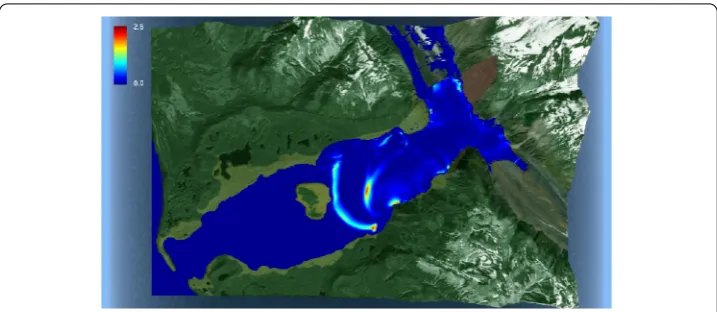
.. D Lituya Bay mega-tsunami
On July , , an . magnitude (rated on the Richter scale) earthquake, along the Fair-weather fault, triggered a major subaerial landslide into the Gilbert Inlet at the head of Lituya Bay on the southern coast of Alaska (USA). The landslide impacted the water at a very high speed generating a giant tsunami with the highest recorded wave run-up in history. The mega-tsunami run-up was up to an elevation of m and caused total de-struction of the forest as well as erosion down to the bedrock on a spur ridge, along the slide axis. Many attempts have been made to understand and simulate this mega tsunami. The aim of this section is to produce a realistic, detailed and accurate simulation of the Lituya Bay mega tsunami of , while taking into account uncertainties in critical pa-rameters such as ratio of layer densities, interlayer friction and Coulomb friction angle. We use public domain topo-bathymetric data as well as the review paper [] to approximate the Gilbert inlet topo-bathymetry.
We consider the system () discretized with a first order path-conservative scheme ()-() whose viscosity matrixQijis defined using the IFCP scheme described in []. Friction terms are discretized semi-implicitly as in [] For simplicity, we use the first-order IFCP scheme. For fast computations, this scheme has been implemented on GPUs using CUDA. This two-dimensional scheme and its GPU adaptation and implementation using single numerical precision are described in detail in []. The MLMC-FV implementation has also been developed in CUDA, where all the updates of the means and variances have also been implemented using CUDA kernels.
A rectangular grid of ,×, = ,, cells with a resolution of m×. m has been designed in order to perform this simulation. We compute with the first order MLMC-FV-IFCP method withL= levels of resolution andM= samples for the high-est level, which corresponds to the grid of ,, cells and constitutes the finhigh-est mesh. We allow a %of variability in the parameterscf,randδ. The mean values of these parameters arecf = .,r= . andδ= ◦. The CFL number is .. Figures , , , show the mean solution and variance for s and s.
The maximum run-up is reached at s. We can see in Figures and that the southern propagating part of the initial wave reaches a maximum mean height of - m with a maximum standard deviation of - m.
While the initial wave moves through the main axis of Lituya Bay, a larger second wave appears as reflection of the first one from the south shoreline. (see Figures and ). These waves sweep both sides of the shoreline in their path. In the north shoreline, the wave reaches between - m height while in the south shoreline the wave reaches mean values between - m assuming a standard deviation of .-. m height.
Figure 4 Mean of the solution att= 39 s.
Figure 5 Variance of the solution att= 39 s.
Figure 6 Mean of the solution att= 120 s.
Figure 7 Variance of the solution att= 120 s.
moderately sensitive to the three uncertain parameters. Thus, it enhances our confidence in previously reported numerical simulations of this event [].
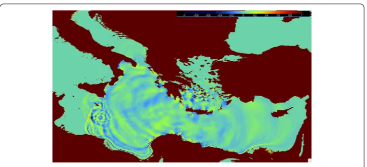
6.2 Earthquake generated tsunami at the Mediterranean Sea
We consider in this section an example of UQ in tsunamis generated by a earthquake. We suppose that the dip, strike and rake angle, and the slip parameter are uncertain. The computational domain is the Western Mediterranean and the epicenter of the earthquake is located in the Ionian Sea. We use the Okada’s model to determine the seafloor defor-mation and the initial condition for the shallow-water system (). Uncertainty in input values for these parameters leads to uncertainty in the solution of the Okada’s model and the shallow-water system (). Here we consider a second order discretization of system () over the sphere by means of a PVM path-conservative scheme in combination with a MUSCL type reconstruction operator. As in the Lituya Bay example, this model has been implemented on GPUs using CUDA as well as the MLMC-FV method. A rectangular grid of arc-sec resolution has been used to perform the simulation with ,, cells and we useL= level of resolution withM= samples for the highest level. We consider the following variability on the parameters:
• slip= ±m. • dip= °±°. • strike= °±°. • rake= °±°.
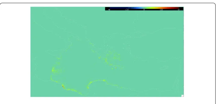
The CFL number is . and the friction coefficient is .. Figures , , , show the mean and variance of the free surface fort= h andt= h, respectively. In this case we see that the computed standard deviation on account of the uncertain parameters is less than . m of the mean on the tsunami propagation. Maximum are located near the coastal areas and in the wave fronts, as expected. Nevertheless, as in the Lituya Bay example, the non-linear evolution has damped the uncertainty.
Figure 8 Mean of the free surface att= 2 h.
Figure 9 Variance of the free surface att= 2 h.
Figure 11 Variance of the solution att= 4 h.
7 Conclusion
Many geophysical flows of interest, such as tsunamis generated by earthquakes, rockslides, avalanches, debris, etc. are modeled by shallow-water type systems. These models are characterized by physical parameters that are usually difficult to determine and that are prone to uncertainty. Consequently, the task of quantifying the resulting solution uncer-tainty (UQ) is of paramount importance in these simulations.
In this paper, we have presented a UQ paradigm by combining a path-conservative finite volume method that can accurately and robustly discretize the underlying non-conservative hyperbolic system () or () together with a Multi-level Monte Carlo sta-tistical sampling algorithm. The algorithm is based on computing on nested sequences of mesh resolutions and estimating statistical quantities by combining results from different resolutions. The method is fully non-intrusive, easy to parallelize, fast and accurate. In particular, one can gain several orders of magnitude in computational efficiency vis a vis the standard Monte Carlo method.
We test the algorithms on a set of numerical examples on real bathymetries. The nu-merical results clearly indicate that the MLMC-FVM framework can approximate statis-tics of quantities of interest such as run-up heights, quite accurately and with reasonable computational cost under efficient implementation on GPUs. There was also qualitative agreement with experimental and observed data. Furthermore, the UQ simulations help in identifying the sensitivity of simulation outputs to the underlying uncertain parame-ters. Thus, they will enable an effective appraisal of sensitivity and enhance risk analysis and hazard mitigation.
The current paper illustrates the power and utility of the MLMC UQ paradigm for tsunami modeling.
Competing interests
The authors declare that they have no competing interests.
Authors’ contributions
Author details
1Dpto. Análisis Matemático, Estadística e Investigación operativa y Matemática Aplicada, University of Málga, Málaga, 29071, Spain.2Dpto. Matemática Aplicada, University of Málga, Málaga, 29071, Spain.3Departement Mathematik, ETH Zürich, Zürich, 8092, Switzerland.
Acknowledgements
This research has been partially supported by the Spanish Government Research project MTM2012-38383-C02-01 and MTM2015-70490-C2-1-R, Andalusian Government Research projects P11-FQM-8179 and P11-RNM-7069 and the Swiss Federal Institute of Technology, ETH (Zurich). The work of SM was partially supported by the ERC STG NN. 306279, SPARCCLE.
Received: 7 January 2016 Accepted: 29 April 2016
References
1. Fritz DJ, Hager WH, Minor H-E. Lituya Bay case: rockslide impact and wave run-up. Sci Tsunami Hazards. 2001;19(1):3-22.
2. Fritz HM, Mohammed F, Yoo J. Lituya Bay landslide impact generated mega-tsunami 50th anniversary. Pure Appl Geophys. 2009;166(1-2):153-75.
3. Okada Y. Surface deformation due to shear and tensile faults in a half space. Bull Seismol Soc Am. 1985;75:1135-54. 4. Yamazaki Y, Cheung KF, Pawlak G, Lay T. Surges along the Honolulu coast from the 2011 Tohoku tsunami. Geophys
Res Lett. 2012;39(9):L09604.
5. Grilli ST, Harris JC, Bakhsh TST, Masterlark TL, Kyriakopoulos C, Kirby JT, Shi FY. Numerical simulation of the 2011 Tohoku tsunami based on a new transient FEM co-seismic source: comparison to far and near-field observations. Pure Appl Geophys. 2013;170(6-8):1333-59.
6. Fernández ED, Bouchut F, Bresch D, Castro MJ, Mangeney A. A new Savage-Hutter type models for submarine avalanches and generated tsunami. J Comput Phys. 2008;227:7720-54.
7. Dal Maso G, Lefloch P, Murat F. Definition and weak stability of nonconservative products. J Math Pures Appl. 1995;74:483-548.
8. Parés C, Muñoz Ruíz ML. On some difficulties of the numerical approximation of nonconservative hyperbolic systems. Bol Soc Esp Mat Apl. 2009;47:23-52.
9. Parés C. Numerical methods for nonconservative hyperbolic systems: a theoretical framework. SIAM J Numer Anal. 2006;44(1):300-21.
10. Che S, Boyer M, Meng J, Tarjan D, Sheaffer JW, Skadron K. A performance study of general-purpose applications on graphics processors using CUDA. J Parallel Distrib Comput. 2008;68:1370-80.
11. Owens JD, Houston M, Luebke D, Green S, Stone JE, Phillips JC. GPU computing. Proc IEEE. 2008;96:879-99. 12. NVIDIA. NVIDIA developer zone. http://developer.nvidia.com/category/zone/cuda-zone.
13. Khronos OpenCL Working Group. The OpenCL specification. http://www.khronos.org/opencl.
14. Fang J, Varbanescu AL, Sips H. A comprehensive performance comparison of CUDA and OpenCL. In: 40th international conference on parallel processing (ICPP 2011). 2011. p. 216-25.
15. Asunción M, Mantas JM, Castro MJ. Simulation of one-layer shallow water systems on multicore and CUDA architectures. J Supercomput. 2011;58:206-14.
16. Brodtkorb AR, Sætra ML, Altinakar M. Efficient shallow water simulations on GPUs: implementation, visualization, verification, and validation. Comput Fluids. 2012;55:1-12.
17. Asunción M, Mantas JM, Castro MJ. Programming CUDA-based GPUs to simulate two-layer shallow water flows. In: Euro-Par 2010 - parallel processing. 2010. p. 353-64. (Lecture notes in computer science; vol. 6272).
18. Castro MJ, Ortega S, Asunción M, Mantas JM, Gallardo JM. GPU computing for shallow water flow simulation based on finite volume schemes. C R, Méc. 2011;339:165-84.
19. Message Passing Interface Forum: A Message Passing Interface Standard. University of Tennessee.
20. Acuña MA, Aoki T. Real-time tsunami simulation on a multi-node GPU cluster [Poster]. In: ACM/IEEE conference on supercomputing 2009 (SC 2009). 2009.
21. Xian W, Takayuki A. Multi-GPU performance of incompressible flow computation by lattice Boltzmann method on GPU cluster. Parallel Comput. 2011;9:521-35.
22. Viñas M, Lobeiras J, Fraguela BB, Arenaz M, Amor M, García JA, Castro MJ, Doallo R. A multi-GPU shallow-water simulation with transport of contaminants. Concurr Comput, Pract Exp. 2012;25:1153-69.
23. Asunción M, Mantas JM, Castro MJ, Fernández-Nieto ED. An MPI-CUDA implementation of an improved Roe method for two-layer shallow water systems. J Parallel Distrib Comput. 2012;72(9):1065-72.
24. Jacobsen DA, Senocak I. Multi-level parallelism for incompressible flow computations on GPU clusters. Parallel Comput. 2013;39:1-20.
25. Bijl H, Lucor D, Mishra S, Schwab C, editors. Uncertainty quantification in computational fluid dynamics. Heidelberg: Springer; 2014. (Lecture notes in computational science and engineering; vol. 92).
26. Chen QY, Gottlieb D, Hesthaven JS. Uncertainty analysis for the steady-state flows in a dual throat nozzle. J Comput Phys. 2005;204:378-98.
27. Poette G, Després B, Lucor D. Uncertainty quantification for systems of conservation laws. J Comput Phys. 2009;228:2443-67.
28. Tryoen J, Le Maitre O, Ndjinga M, Ern A. Intrusive projection methods with upwinding for uncertain non-linear hyperbolic systems. J Comput Phys. 2010;229(18):6485-511.
29. Xiu D, Hesthaven JS. High-order collocation methods for differential equations with random inputs. SIAM J Sci Comput. 2005;27:1118-39.
30. Zabaras N, Ma X. An adaptive hierarchical sparse grid collocation algorithm for the solution of stochastic differential equations. J Comput Phys. 2009;228:3084-113.
32. Mishra S, Schwab C. Sparse tensor multi-level Monte Carlo finite volume methods for hyperbolic conservation laws with random initial data. Math Comput. 2012;280:1979-2018.
33. Giles M. Improved multilevel Monte Carlo convergence using the Milstein scheme. Preprint NA-06/22. Oxford Computing Lab., Oxford, UK; 2006.
34. Giles M. Multilevel Monte Carlo path simulation. Oper Res. 2008;56:607-17.
35. Heinrich S. Multilevel Monte Carlo methods. In: Large-scale scientific computing. Berlin: Springer; 2001. p. 58-67. (Lecture notes in computer science; vol. 2170).
36. Mishra S, Schwab C, Sukys J. Multi-level Monte Carlo finite volume methods for nonlinear systems of conservation laws in multi-dimension. J Comput Phys. 2012;231:3365-88.
37. Mishra S, Schwab C, Sukys J. Multilevel Monte Carlo finite volume methods for shallow water equations with uncertain topography in multi-dimensions. SIAM J Sci Comput. 2012;34(6):761-84.
38. Sánchez-Linares C, Asunción M, Castro MJ, Mishra S, Sukys J. Multi-level Monte Carlo finite volume method for shallow water equations with uncertain parameters applied to landslides-generated tsunamis. Appl Math Model. 2015;39(23-24):7211-26.
39. Bouchut F, Mangeney-Castelnau A, Perthame B, Vilotte JP. A new model of Saint-Venant and Savage-Hutter type for gravity driven shallow water flows. C R Math Acad Sci Paris. 2003;336(6):531-6.
40. Asunción M, Mantas JM, Castro MJ, Ortega S. Scalable simulation of tsunamis generated by submarine landslides on GPU clusters. Accepted on Environ Model Softw. May 2016.
41. Volpert AI. Spaces BV and quasilinear equations. Math USSR Sb. 1967;73:255-302.
42. Castro MJ, Fernández-Nieto ED, Morales de Luna T, Narbona-Reina G, Parés C. A HLLC scheme for nonconservative hyperbolic problems. Application to turbidity currents with sediment transport. ESAIM: Math Model Numer Anal. 2013;47(1):1-32.
43. Castro MJ, Fernández-Nieto ED, Ferreiro AM, García Rodríguez JA, Parés C. High order extensions of Roe schemes for two dimensional nonconservative hyperbolic systems. J Sci Comput. 2009;39(1):67-114.
44. Harten A, Lax PD, van Leer B. On upstream differencing and Godunov type schemes for hyperbolic conservation laws. SIAM Rev. 1983;25:35-61.
45. Degond P, Peyrard P-F, Russo G, Villedieu P. Polynomial upwind schemes for hyperbolic systems. C R Acad Sci Paris Ser I. 1999;328:479-83.
46. Castro MJ, Fernández-Nieto ED. A class of computationally fast first order finite volume solvers: PVM methods. SIAM J Sci Comput. 2012;34:A2173-96.
47. Castro MJ, Gallardo JM, Marquina A. A class of incomplete Riemann solvers based on uniform rational approximations to the absolute value function. J Sci Comput. 2014;60(2):363-89.
48. Castro MJ, LeFloch PG, Muñoz ML, Parés C. Why many theories of shock waves are necessary: convergence error in formally path-consistent schemes. J Comput Phys. 2008;3227:8107-29.
49. Hou TY, LeFloch PG. Why nonconservative schemes converge to wrong solutions: error analysis. Math Comput. 1994;62:497-530.
50. Muñoz ML, Parés C. On the convergence and well-balanced property of path-conservative numerical schemes for systems of balance laws. J Sci Comput. 2011;48:274-95.
51. van Leer B. Towards the ultimate conservative difference scheme. V. A second order sequel to Godunov’s method. Comput Phys. 1979;32:101-36.
52. Gottlieb S, Shu CW. Total variation diminishing Runge-Kutta schemes. Math Comput. 1998;67:73-85.
53. Matsumoto M, Nishimura T. Mersenne twister: a 623-dimensionally equidistributed uniform pseudo-random number generator. ACM Trans Model Comput Simul. 1998;8(1):3-30.
54. Fernández-Nieto ED, Castro MJ, Parés C. On an intermediate field capturing Riemann solver based on a parabolic viscosity matrix for the two-layer shallow water system. J Sci Comput. 2011;48(1-3):117-40.
55. Miller DJ. Giant waves in Lituya Bay, Alaska: a timely account of the nature and possible causes of certain giant waves, with eyewitness reports of their destructive capacity. Professional paper; 1960.