System of generalized mixed equilibrium problems, variational inequality, and fixed point problems

(1)

R E S E A R C H

Open Access

System of generalized mixed equilibrium

problems, variational inequality, and ﬁxed

point problems

Morad Ali Payvand and Sedigheh Jahedi

*

*_{Correspondence:}

[email protected]

Department of Mathematics, Shiraz University of Technology, Shiraz, 71555-313, Iran

Abstract

The purpose of this paper is to introduce a new iterative algorithm for finding a common element of the set of solutions of a system of generalized mixed equilibrium problems, the set of common fixed points of a finite family of pseudo contraction mappings, and the set of solutions of the variational inequality for an inverse strongly monotone mapping in a real Hilbert space. We establish results on the strong convergence of the sequence by the proposed scheme to a common element of the above three solution sets. These results extend and improve some corresponding results in this area. Finally, we give a numerical example which supports our main theorem.

MSC: 47H10; 47H09; 65K10

Keywords: generalized mixed equilibrium problem; variational inequality problem; strictly pseudo contraction mapping

1 Introduction

Letbe a bifunction fromK×Kinto the set of real numbers,R, whereKis a nonempty closed convex subset of a real Hilbert spaceH. The equilibrium problem is to ﬁnd a point x∈Ksuch that

(x,y)≥, ∀y∈K. (.)

We denote the set of solutions of (.) by EP(). The equilibrium problem includes the ﬁxed point problem, the variational inequality problem, the optimization problem, the saddle point problem, the Nash equilibrium problem and so on, as its special cases [, ].

The generalized mixed equilibrium problem is to ﬁnd a pointx∈Ksuch that

(x,y) +Ax,y–x+ϕ(y) –ϕ(x)≥, ∀y∈K, (.)

whereϕis a function onKintoRandAis a nonlinear mapping fromKtoH. The set of solutions of a generalized mixed equilibrium problem is denoted byGMEP(,A,ϕ).

(2)

If we consider=  andϕ=  in (.), then we have the classical variational inequality problem which is to ﬁnd a pointx∈Ksuch that

Ax,y–x ≥, ∀y∈K. (.)

The solution set of (.) is denoted byVI(K,A).

To proceed we need to recall some deﬁnitions and concepts.

Deﬁnition . LetKbe a nonempty closed convex subset of a real Hilbert spaceH.

(i) A mappingS:K→Kis called nonexpansive ifSx–Sy ≤ x–y, for allx,y∈K. (ii) A mappingT:K→Kis calledk-strict pseudo contractive mapping, if for all

x,y∈Kthere exists a constant≤k< such that

Tx–Ty≤ x–y+k(I–T)x– (I–T)y, ∀x,y∈K, (.)

whereIis the identity mapping onK.

(iii) A mappingA:H→His called monotone if for eachx,y∈H,

Ax–Ay,x–y ≥.

(iv) A mappingA:H→His calledβ-inverse strongly monotone if there existsβ> 

such that

Ax–Ay,x–y ≥βAx–Ay, ∀x,y∈H.

(v) The mappingA:K→HisL-Lipschitz continuous if there exists a positive real numberLsuch thatAx–Ay ≤Lx–yfor allx,y∈H. If <L< , then the mappingAis a contraction with constantL.

Clearly a nonexpansive mapping is a -strict pseudo contractive mapping []. Note that in a Hilbert space, (.) is equivalent to the following inequality:

Tx–Ty,x–y ≤ x–y– –k

 (x–y) – (Tx–Ty)



, ∀x,y∈K. (.)

We denoteF(T) ={x∈K:Tx=x}, the set of ﬁxed points ofT. It can be shown that, for ak-strict pseudo contractive mappingT:K→K, the mappingI–T is demiclosed,i.e., if{xn}is a sequence inKwithxnqandxn–Txn→, thenq∈F(T) (refer to []). The

symbolsand→denote weak and strong convergence, respectively.

A set valued mappingQ:H→H_{is called monotone if for all}_x,_y_∈_H,_f _∈_{Q(x) and} g ∈Q(y) implyx–y,f –g ≥. A monotone mappingQ:H→H _{is maximal if the} graphG(Q) ofQis not properly contained in the graph of any other monotone mapping. It is well known that a monotone mappingQis maximal if and only if for (x,f)∈H×H,

x–y,f –g ≥ for every (y,g)∈G(Q) impliesf∈Q(x) [].

For anyx∈Hthere exists a unique point inKdenoted byPKxsuch thatx–PKx ≤

(3)

PKx∈Kandx–PKx,PKx–y ≥, for ally∈K. It is also known thatPKx–PKy≤

x–y,PKx–PKy, for allx,y∈K[]. In the context of the variational inequality problem, we obtain

q∈VI(K,A) if and only if q=PK(q–λAq), ∀λ> . (.)

LetIbe an index set. For eachi∈I, letibe a real valued bifunction onK×K,Aia nonlinear mapping, andϕi:K→Ra function. The system of generalized mixed equilib-rium problems as an extension of problems (.), (.), and (.) is to ﬁnd a pointx∈K such that

i(x,y) +Aix,y–x+ϕi(y) –ϕi(x)≥, ∀y∈K,∀i∈I. (.)

Note that_i_∈_IGMEP(i,Ai,ϕi) is the solution set of (.).

Vast range of problems which arise in economics, finance, image reconstruction, trans-portation, network and so on, appear as a special case of problem (.); see for example [– ]. This problem also covers various forms of feasibility problems. So, it seems reasonable to study the system of generalized mixed equilibrium problems. There are many authors who introduced some iterative processes for finding the solution set of these problems or common solution of someone with others, for instance see [, –] and the references therein. In , Penget al.[] introduced the following iterative algorithm for finding a common element of fixed points of a family of infinite nonexpansive mappings and the set of solutions of a system of finite family of equilibrium problems:

⎧ ⎪ ⎪ ⎪ ⎨ ⎪ ⎪ ⎪ ⎩

z=z∈H,

un=TβFnmT

Fm–

βn · · ·T

F

βnT

F

βnzn,

vn=PK(I–snA)un,

zn+=αnγf(Wnzn) + (I–αnB)WnPK(I–rnA)vn.

Under suitable conditions, they presented and proved a strong convergence theorem for ﬁnding an element of =∞_i_=F(Ti)∩VI(K,A)∩

m

k=EP(Fk). In , Cai and Bu [] proposed an iterative method as follows:

⎧ ⎪ ⎪ ⎪ ⎨ ⎪ ⎪ ⎪ ⎩

x=x∈K,

zn=Tr(MFM,n,ϕM)(I–rM,nBM)T

(FM–,ϕM–)

rM–,n (I–rM–,nBM–)· · ·T (F,ϕ)

r,n (I–rB)xn,

un=PK(I–λN,nAN)PK(I–λN–,nAN–)· · ·PK(I–λ,nA)zn, xn+=αnf(Snxn) +βnxn+ (I–βn–αn)W(τn)Sun.

They proved that under appropriate conditions, the sequences{xn},{zn}, and{un} con-verge strongly to z=P f(z), where =F(W)∩∞_i_=F(Ti)∩

m

k=GMEP(Fk,ϕk,Bk)∩

N

(4)

family of nonexpansive mappings, and the set of solutions of the variational inequality of anα-inverse strongly monotone mapping in a real Hilbert space:

⎧ ⎪ ⎪ ⎪ ⎨ ⎪ ⎪ ⎪ ⎩

φ(un,y) +_r_ny–un,un–xn ≥, wn=αnxn+ ( –αn)WnPK(un–λnAun), Kn+={z∈Kn:wn–z ≤ xn–z}, xn+=PKn+(x).

He showed that under suitable conditions, the above algorithm strongly converges to

N

i=F(Ti)∩EP(φ)∩VI(K,A), where for eachi= , . . . ,N,Tiis a nonexpansive mapping andAis anα-inverse strongly monotone mapping.

In this paper, we present an iterative algorithm for finding a common solution of a sys-tem of finite generalized mixed equilibrium problems, a variational inequality problem for an inverse strongly monotone mapping and common fixed points of a finite family of strictly pseudo contractive mappings. We show that the algorithm strongly converges to a solution of the problem under certain conditions. Our results modify, improve and extend corresponding results of Takahashi and Takahashi [], Zhanget al.[], Shehu [], Thianwan [], and others. The rest of the paper is organized as follows. Section  briefly explains the necessary mathematical background. Section  presents the main re-sults. A numerical example is provided in the final section.

2 Preliminaries

It is well known that in a (real) Hilbert spaceH

x+y≤ x+ y,x+y, (.)

for allx,y∈H[]. Furthermore, it is easy to see that

m

i=

xi



= m

i,j=

xi,xj. (.)

Lemma .([]) Let{an},{bn},and{cn}be three nonnegative real sequences satisfying

an+≤( –tn)an+bn+cn

with{tn} ⊂[, ], ∞n=tn=∞,bn=o(tn),and ∞n=cn<∞.Thenlimn→∞an= .

Lemma .([]) Let H be a(real)Hilbert space and{xn}Nn=be a bounded sequence in H.

Let{an}Nn=be a sequence of real numbers such that Nn=an= .Then

N

i=

aixi



≤

N

i=

aixi.

Lemma .([]) Let{xn}and{zn}be bounded sequences in a Banach space andβnbe a sequence of real numbers such that <lim infn→∞βn<lim supn→∞βn< for all n≥. Suppose that xn+= ( –βn)zn+βnxnfor all n≥andlim supn→∞(zn+–zn–xn+–

(5)

Let us assume that the bifunctionsatisﬁes the following conditions:

(A) (x,x) = ,∀x∈K;

(A) is monotone onK,i.e.,(x,y) +(y,x)≤,∀x,y∈K; (A) for allx,y,z∈K,limt→+(tz+ ( –t)x,y)≤(x,y);

(A) for allx∈K,y→(x,y)is convex and lower semicontinuous.

Lemma .([]) Let K be a nonempty closed convex subset of Hilbert space H andbe a real valued bifunction on K×K satisfying(A)-(A).Let r> and x∈H,then there exists z∈K such that

(z,y) +

ry–z,z–x ≥, ∀y∈K.

Lemma .([]) Suppose all conditions in Lemma.are satisﬁed.For any given r> , deﬁne a mapping Tr:H→K as

Trx=

z∈K:(z,y) +

ry–z,z–x ≥,∀y∈K

,

for all x∈H.Then the following conditions hold:

. Tris single valued;

. Tris ﬁrmly nonexpansive,i.e.,

Trx–Try≤ Trx–Try,x–y, ∀x,y∈H;

. F(Tr) =EP();

. EP()is a closed and convex set.

Remark . For the generalized mixed equilibrium problem (.), if the nonlinear opera-torAis a monotone, Lipschitz continuous mapping,ϕis a convex and lower semicontin-uous function, and the real valued bifunctionadmits the conditions (A)-(A), then it is easy to show thatG(x,y) =(x,y) +Ax,y–x+ϕ(y) –ϕ(x) also satisﬁes the conditions (A)-(A), and the generalized mixed equilibrium (.) is still the following equilibrium problem:

ﬁnd x∈K such that G(x,y)≥, ∀y∈K.

3 Main results

As is well known, the strict pseudo contraction mappings have more useful applications than nonexpansive mappings like in solving inverse problems []. In addition, various problems reduced to find the common element of the fixed point set of a family of nonlin-ear mappings such as image restoration (see for example []). For construction an algo-rithm which can used to obtain the fixed point set of a family of strictly pseudo contractive mappings we need to introduce the following proposition.

In the sequel,I={, , . . . ,m}andJ={, , . . . ,l}are two index sets.

(6)

l

j=γj= .Ifγ∈[k, )such that k=max{k, . . . ,kl},then S is a nonexpansive mapping and F(S) =_j_∈_JF(Tj).

Proof By the deﬁnition of the mappingS, we have

Sx–Sy=γ_x–y+ j∈J

γj(Tjx–Tjy)



+ γ

j∈J

γjx–y,Tjx–Tjy. (.)

On the other hand, from (.) and (.) we have

j∈J

γj(Tjx–Tjy)

 =

j,i∈J

γjγiTjx–Tjy,Tix–Tiy

≤

j,i∈J

γjγiTjx–TjyTix–Tiy

≤ 



j,i∈J

γjγi

Tjx–Tjy+Tix–Tiy

≤ 



j,i∈J

γjγi

x–y+kj(x–y) – (Tjx–Tjy)



+x–y+ki(x–y) – (Tix–Tiy)



=

j,i∈J

γjγix–y

+

j∈J

γj

i∈J

γikj(x–y) – (Tjx–Tjy). (.)

Furthermore, (.) implies that, for eachj∈J,

x–y,Tjx–Tjy ≤ x–y–  –kj

 (x–y) – (Tjx–Tjy)



. (.)

By substituting (.) and (.) in (.), we have

Sx–Sy≤

γ_+ j,i∈J

γjγi+ 

j∈J

γγj

x–y

+

j∈J

γj

i∈J

γikj(x–y) – (Tjx–Tjy)



–

j∈J

γγj( –kj)(x–y) – (Tjx–Tjy)

=x–y–

j∈J

γj

γ( –kj) –

i∈J

γikj

(x–y) – (Tjx–Tjy)



=x–y–

j∈J

γj

γ( –kj) – ( –γ)kj(x–y) – (Tjx–Tjy)

(7)

=x–y– j∈J

γj(γ–kj)(x–y) – (Tjx–Tjy)



≤ x–y– j∈J

γj(γ–k)(x–y) – (Tjx–Tjy)



≤ x–y. (.)

ThenSis a nonexpansive mapping. Now, by the deﬁnition ofSwe obtainI–S= _j_∈_Jγj(I– Tj) and clearlyF(S) =

j∈JF(Tj).

Theorem . Leti:K×K→R,i∈I,be bifunctions satisfying(A)-(A).Suppose that, for each i∈I,the Biareθi-inverse strongly monotone mappings,the Ciare monotone and Lipschitz continuous mappings from K into H,and theϕiare convex and lower semicon-tinuous functions from K into R.Let Tj:K→K,j∈J,be kj-strict pseudo contractive map-pings and A:K→H be a σ-inverse strongly monotone mapping. Let f :K→K be an

ε-contraction mapping and{vn}be a convergent sequence in K with limit point v.Suppose that =_i_∈_IGMEP(i,Bi,Ci,ϕi)∩

j∈JF(Tj)∩VI(A,K)is nonempty.For any initial guess x∈K,deﬁne the sequence{xn}by

⎧ ⎪ ⎪ ⎪ ⎪ ⎨ ⎪ ⎪ ⎪ ⎪ ⎩

i(un,i,y) +Ciun,i+Bixn,y–un,i+ϕi(y) –ϕi(un,i) +_r

n,iy–un,i,un,i–xn ≥, ∀y∈K,∀i∈I,

yn=αnvn+ (I–αn(I–f))PK( i∈Iδn,iun,i–λnA i∈Iδn,iun,i), xn+=βnxn+ ( –βn)(γI+ j∈JγjTj)PK(yn–λnAyn),

(.)

where for all n∈N,{λn},{rn,i}i∈I ⊆(,∞), and{αn},{βn},{δn,i}i∈I,{γj}j∈J ⊆(, ) are se-quences satisfying the following control conditions:

. limn→∞αn= , ∞n=αn=∞;

.  <lim infn→∞βn≤lim supn→∞βn< ;

. for somea,b∈(, σ),λn∈[a,b]andlimn→∞|λn+–λn|= ;

. for somed> , <d≤δn,i≤, i∈Iδn,i= and ∞n=|δn+,i–δn,i|<∞;

. for somec> ,k≤γ≤c< such thatk=maxj∈J{kj}and j∈Jγj= ;

. for someτi,ρi∈(, θi),rn,i∈[τi,ρi]and ∞n=|rn+,i–rn,i|<∞,i∈I. Then the sequences{xn}converges strongly to z∈ ,where z=P (v+f(z)).

Proof Forx,y∈Kandi∈I, putGi(x,y) =i(x,y)+Cix,y–x+ϕi(y)–ϕi(x). By Remark ., Gisatisﬁes the conditions (A)-(A) and so the algorithm (.) can be rewritten as fol-lows:

⎧ ⎪ ⎨ ⎪ ⎩

Gi(un,i,y) +Bixn,y–un,i+_r_n_,_iy–un,i,un,i–xn ≥, ∀y∈K,i∈I, yn=αnvn+ (I–αn(I–f))PK( i∈Iδn,iun,i–λnA i∈Iδn,iun,i),

xn+=βnxn+ ( –βn)(γI+ j∈JγjTj)PK(yn–λnAyn).

(.)

Claim  The sequences{xn},{yn},{un},{tn},and{kn}are bounded where,for each n∈N, un= i∈Iδn,iun,i,tn=PK(yn–λnAyn),and kn=PK(un–λnAun).

To prove the claim from (.) we have

Gi(un,i,y) +  rn,i

y–un,i,un,i– (I–rn,iBi)xn

(8)

Then, by using Lemma ., for eachi∈I, we haveun,i=Trn,i(xn–rn,iBixn), and, for any

q∈ ,q=Trn,i(q–rn,iBiq). Thus

un,i–q=Trn,i(xn–rn,iBixn) –Trn,i(q–rn,iBiq) 

≤(xn–rn,iBixn) – (q–rn,iBiq)

≤ xn–q+rn,iBixn–Biq– rn,ixn–q,Bixn–Biq

≤ xn–q+rn,iBixn–Biq– rn,iθiBixn–Biq

=xn–q+rn,i(rn,i– θi)Bixn–Biq

≤ xn–q. (.)

So, we have

un–q≤

i∈I

δn,iun,i–q≤

i∈I

δn,ixn–q=xn–q. (.)

By the deﬁnition oftnandknwe have

tn–q ≤(yn–λnAyn) – (q–λnAq)

≤ yn–q (.)

and

kn–q ≤(un–λnAun) – (q–λnAq)

≤ un–q. (.)

Sincelim_n_→∞vn=v,{vn}is bounded,

yn–q ≤αnvn–q+αnf(kn) –q+ ( –αn)kn–q

≤αnM+αnεkn–q+αnf(q) –q+ ( –αn)xn–q

= –αn( –ε)

xn–q+αn

M+f(q) –q

≤max

xn–q,   –ε

M+f(q) +q

, (.)

whereM=supn≥{vn–q}. PuttingS=γI+ j∈JγjTj, by Proposition .,Sis nonex-pansive. On the other hand, for alln∈N, we have

xn+–q ≤βnxn–q+ ( –βn)Stn–q

≤βnxn–q+ ( –βn)tn–q

≤βnxn–q+ ( –βn)yn–q

≤max

xn–q,   –ε

M+f(q) +q

(9)

By induction, we deduce that

xn+–q ≤max

x–q,

  –ε

M+f(q) +q

, ∀n∈N. (.)

Therefore,{xn}is bounded, and so are{yn},{un},{un,i},{tn}, and{kn}.

Claim  xn+–xn →as n→ ∞.

Letzn=_–βnxn+–

βn

–βnxn. Hence

zn+–zn=

_{ –}_β_n_+(xn+–βn+xn+) –

  –βn

(xn+–βnxn)

=Stn+–Stn

≤ tn+–tn. (.)

Now, by the deﬁnition oftnwe have

tn+–tn ≤(yn+–λn+Ayn+) – (yn–λnAyn)

≤ yn+–yn+|λn+–λn|Ayn. (.)

Similarly,

kn+–kn ≤ un+–un+|λn+–λn|Aun. (.)

By (.) and the deﬁnition ofynwe obtain

yn+–yn ≤αn+μvn+–vn+|αn+–αn|vn+|αn+–αn|f(kn)

+|αn+–αn|kn+I–αn+(I–f)

(kn+) –

I–αn+(I–f)

(kn)

≤αn+vn+–vn+|αn+–αn|

vn+f(kn)+kn

+ –αn+( –ε)

kn+–kn

≤αn+vn+–vn+|αn+–αn|

vn+f(kn)+kn

+ –αn+( –ε)

un+–un+|λn+–λn|Aun

. (.)

Furthermore, by the deﬁnition ofun,

un+–un=

i∈I

(δn+,iun+,i–δn,iun,i)

≤

i∈I

δn+,i(un+,i–un,i)

+

i∈I

(δn+,i–δn,i)un,i

≤

i∈I

δn+,iun+,i–un,i+

i∈I

(10)

From (.), since for eachi∈I,un,i,un+,i∈K,

Gi(un+,i,un,i) +  rn+,i

un,i–un+,i,un+,i– (I–rn+,iBi)xn+

≥ (.)

and

Gi(un,i,un+,i) +  rn,i

un+,i–un,i,un,i– (I–rn,iBi)xn

≥. (.)

By adding the two inequalities (.), (.), and the monotonicity ofGiwe have

un+,i–un,i,

un,i– (I–rn,iBi)xn rn,i

–un+,i– (I–rn+,iBi)xn+ rn+,i

≥, ∀i∈I.

So

un+,i–un,i,un,i– (I–rn,iBi)xn–rn,iBixn+–

rn,i rn+,i

(un+,i–xn+)

≥, ∀i∈I.

Thus, for eachi∈I,

un+,i–un,i, (I–rn,iBi)xn+– (I–rn,iBi)xn+ (un,i–un+,i) +

 – rn,i rn+,i

(un+,i–xn+)

≥.

This yields

un+,i–un,i≤

un+,i–un,i, (I–rn,iBi)xn+– (I–rn,iBi)xn

+

 – rn,i rn+,i

(un+,i–xn+)

≤ un+,i–un,i

(I–rn,iBi)xn+– (I–rn,iBi)xn

+ – rn,i rn+,i

un+,i–xn+

≤ un+,i–un,i

xn+–xn+

 – rn,i

rn+,i

un+,i–xn+

, ∀i∈I,

or

un+,i–un,i ≤ xn+–xn+  rn+,i|

rn+,i–rn,i|un+,i–xn+

≤ xn+–xn+ 

τ|rn+,i–rn,i|M, ∀i∈I, (.)

whereτ=infn≥{rn,i}andM=supn≥{un,i–xn}. Thus, from (.), (.), (.), (.), and (.) we obtain

zn+–zn ≤ xn+–xn+αn+vn+–vn

+|αn+–αn|

(11)

+|λn+–λn|Ayn+

 –αn+( –ε)

i∈I

δn+,i 

τ|rn+,i–rn,i|M

+|λn+–λn|Aun+

i∈I

|δn+,i–δn,i|un,i

.

So, by assumptions - of the theorem

lim sup

n→∞

zn+–zn–xn+–xn

≤,

and by Lemma ., we have

lim

n→∞zn–xn= .

But, sincexn+–xn= ( –βn)(zn–xn), we have

lim

n→∞xn+–xn= . (.)

Claim  limn→∞xn–Sxn= .

Note that

xn–Sxn ≤ xn+–xn+xn+–Stn+Stn–Sxn

≤ xn+–xn+xn+–Stn+tn–xn. (.)

First we show thatlimn→∞xn+–Stn= . From (.)

xn+–Stn ≤βnxn–Stn

≤βnxn–xn++βnxn+–Stn.

Hence

xn+–Stn ≤

βn  –βn

xn–xn+.

This implies that

lim

n→∞xn+–Stn= . (.)

Now, we prove thatlimn→∞tn–xn= . To do this, it suﬃces to show thatlimn→∞xn– un=  andlimn→∞un–tn= . By the deﬁnition oftnwe have

tn–q≤(yn–λnAyn) – (q–λnAq)



≤ yn–q+λn(λn– σ)Ayn–Aq

(12)

So, by (.) and the convexity of · _{, we have}

xn+–q≤βnxn–q+ ( –βn)Stn–q

≤βnxn–q+ ( –βn)tn–q

≤βnxn–q+ ( –βn)

xn–q+λn(λn– σ)Ayn–Aq

=xn–q+ ( –βn)λn(λn– σ)Ayn–Aq.

Hence

( –βn)λn(σ–λn)Ayn–Aq≤ xn–q–xn+–q ≤ xn–xn+

xn–q+xn+–q

,

and then

lim

n→∞Ayn–Aq= . (.)

Using the projection properties gives us

tn–q =PK(yn–λnAyn) –PK(q–λnAq)



≤(yn–λnAyn) – (q–λnAq),tn–q

= 

(yn–λnAyn) – (q–λnAq)



+tn–q

–(yn–λnAyn) – (q–λnAq) – (tn–q)



≤ 



yn–q+tn–q–yn–tn–λn(Ayn–Aq)

≤ 



yn–q+tn–q–yn–tn–λnAyn–Aq

+ λnyn–tn,Ayn–Aq

.

This implies that

tn–q≤ yn–q–yn–tn–λnAyn–Aq

≤ yn–q–yn–tn+ λnyn–tn,Ayn–Aq. (.)

From (.) and the convexity of · _{, one can see that, for}_q_∈ _,

≤βnxn–q+ ( –βn)

yn–q–yn–tn

(13)

≤βnxn–q+ ( –βn)

αnvn–q+αnf(kn) –q



+ ( –αn)kn–q–yn–tn+ λnyn–tn,Ayn–Aq

≤βnxn–q+ ( –βn)



+ ( –αn)xn–q–yn–tn+ λnyn–tn,Ayn–Aq

.

Hence

( –βn)yn–tn≤( –βn)



+xn–q–xn+–q ≤( –βn)



+ λnyn–tnAyn–Aq

+xn–xn+

xn–q+xn+–q

,

and so by (.)

lim

n→∞yn–tn= . (.)

Next, we show thatlim_n_→∞yn–un= . The deﬁnition ofknand a similar argument to (.) give us

kn–q≤ xn–q+λn(λn– σ)Aun–Aq. (.)

Then

≤βnxn–q+ ( –βn)yn–q

≤βnxn–q+ ( –βn)

αnvn–q

+αnf(kn) –q



+ ( –αn)kn–q

≤ xn–q+ ( –βn)

αnvn–q+αnf(kn) –q

+ ( –βn)( –αn)λn(λn– σ)Aun–Aq.

Hence

( –βn)( –αn)λn(σ–λn)Aun–Aq≤ xn–q–xn+–q ≤ xn–xn+

xn–q+xn+–q

,

and therefore

lim

(14)

Similar to (.) we can see that

kn–q ≤ un–q–un–kn+ λnun–kn,Aun–Aq

≤ xn–q–un–kn+ λnun–kn,Aun–Aq. (.)

From (.) and the convexity of · _{, we have}

≤βnxn–q+ ( –βn)

αnvn–q

+αnf(kn) –q



+ ( –αn)kn–q

≤βnxn–q+ ( –βn)



+ ( –αn)

xn–q–un–kn+ λnun–kn,Aun–Aq

≤ xn–q+ ( –βn)



+ ( –αn)λnun–kn,Aun–Aq

– ( –βn)( –αn)un–kn.

So

( –βn)( –αn)un–kn≤( –βn)



+ ( –βn)( –αn)λnun–kn,Aun–Aq

+xn–q–xn+–q ≤( –βn)



+ ( –βn)( –αn)λnun–knAun–Aq

+xn–xn+

xn–q+xn+–q

.

Then the above inequality and (.) imply that

lim

n→∞un–kn= . (.)

But from (.),

yn–un ≤αnvn–un+αnf(kn) –un+ ( –αn)kn–un.

So, from (.) we have

lim

n→∞yn–un= . (.)

Then by (.) and (.) we have

lim

(15)

Now, we show thatlimn→∞xn–un= . To do this, note that, for anyi∈I,

un,i–q =Trn,i(xn–rn,iBixn) –Trn,i(q–rn,iBiq) 

≤Trn,i(xn–rn,iBixn) –Trn,i(q–rn,iBiq), (xn–q) –rn,i(Bixn–Biq)

=un,i–q,xn–q–rn,iun,i–q,Bixn–Biq

≤ un,i–q,xn–q–rn,iθiBixn–Biq

≤ un,i–q,xn–q. (.)

So, from (.) and the deﬁnition ofun, we obtain

un–q≤

i∈I

δn,iun,i–q

≤

i∈I

δn,iun,i–q,xn–q

=

i∈I

δn,iun,i–q,xn–q

=un–q,xn–q

≤ 



un–q+xn–q–un–xn

.

Thus,

un–q≤ xn–q–un–xn. (.)

SinceSis nonexpansive, we have

≤βnxn–q+ ( –βn)



+ ( –βn)( –αn)kn–q

≤βnxn–q+ ( –βn)



+ ( –βn)( –αn)un–q

≤βnxn–q+ ( –βn)



+ ( –βn)( –αn)

xn–q–xn–un

.

Hence

( –βn)( –αn)xn–un≤( –βn)



(16)

≤( –βn)



+xn–q–xn+–q

xn–q+xn+–q

≤( –βn)

αnvn–q+αnf(kn) –q

+xn–q+xn+–q

xn–xn+,

which yields

lim

n→∞xn–un= . (.)

Sincetn–xn ≤ tn–un+un–xn, from (.) and (.) we obtain

lim

n→∞tn–xn= . (.)

Inequality (.) and equations (.), (.), andxn–xn+ → imply that

lim

n→∞xn–Sxn= . (.)

Claim  lim sup_n_→∞v+f(z) –z,yn–z ≤,where z=P (v+f(z)).

To prove the claim, let{ynk}be a subsequence of{yn}such that

lim sup

n→∞

v+f(z) –z,yn–z

=lim sup

n→∞

v+f(z) –z,ynk–z

. (.)

By boundedness of{ynk}, there exists a subsequence of{ynk}which is weakly convergent

toz∈K. Without loss of generality, we can assume thatynkz. So, (.) reduces to

lim sup

n→∞

=v+f(z) –z,z–z

. (.)

Therefore, by projection properties, to provev+f(z) –z,z–z ≥, it suﬃces to show

thatz∈ .

(a) First we prove thatz∈ m

j∈JF(Tj). From (.) and the demiclosedness property of Swe obtainz∈F(S). So, by Proposition .,z∈

m j∈JF(Tj).

(b) Next we show thatz∈VI(A,K). Note that from boundedneess of{xn},{un}, and equation (.), there exist subsequences{xnk}and{unk} of{xn} and{un}, respectively,

which converge weakly toz. Suppose thatNKxis a normal cone toK atxandQis a mapping deﬁned by

Q(x) =

Ax+NKx, x∈K,

∅, x∈/K. (.)

It is well known that Q is a maximal monotone mapping and ∈Q(x) if and only if

x∈VI(A,K). For details see []. If (x,u)∈G(Q), thenu–Ax∈NKx. Sincekn=PK(un–

λnAun)∈K, we have

(17)

In addition, from projection properties we havex–kn,kn– (un–λnAun) ≥. Thenx– kn,kn_λ–_nun+Aun ≥. Hence, from (.) we have

x–knk,u ≥ x–knk,Ax

≥ x–knk,Ax–

x–knk,

knk–unk λnk

+Aunk

=x–knk,Ax–Aknk+x–knk,Aknk–Aunk

–

x–knk,

≥ x–knk,Aknk–Aunk–

x–knk,

. (.)

SinceAis a continuous mapping, from (.) and (.) we deduce that

x–z,u ≥, ask→ ∞.

Therefore, from maximal monotonicity ofQ, we obtain ∈Q(z) and hencez∈VI(A,K).

(c) Now we prove thatz∈i∈IGEP(Gi,Bi). For alli∈I, by (.),

un,i–q≤ un,i–q,xn–q

≤



un,i–q+xn–q–un,i–xn

and then

un,i–q≤ xn–q–un,i–xn.

This implies that

un–q≤

i∈I

δn,iun,i–q

≤ xn–q–

i∈I

δn,iun,i–xn.

Therefore, for anyi∈I,

un,i–xn≤

i∈I

δn,iun,i–xn≤ xn–q–un–q

≤ xn–un

xn–q+un–q

.

So by (.),

lim

n→∞un,i–xn= , ∀i∈I. (.)

Since{un,i}i∈I is bounded, by (.), there exists a weakly convergent subsequence{unk,i}

(18)

un,i=Trn,i(xn–rn,iBixn), for ally∈Kwe have

Gi(un,i,y) +Bixn,y–un,i+  rn,i

y–un,i,un,i–xn ≥, ∀i∈I.

From (A) we obtain

Bixn,y–un,i+  rn,i

y–un,i,un,i–xn ≥Gi(y,un,i), ∀y∈K,∀i∈I.

Hence, for ally∈K,

Bixnk,y–unk,i+

y–unk,i,

unk,i–xnk

rnk,i

≥Gi(y,unk,i), ∀i∈I. (.)

Letyt=ty+ ( –t)z, wheret∈(, ] andy∈K. Thenyt∈Kand by (.),

yt–unk,i,Biyt ≥ yt–unk,i,Biyt–yt–unk,i,Bixnk

–

yt–unk,i,

unk,i–xnk

rnk,i

+Gi(yt,unk,i)

=yt–unk,i,Biyt–Biunk,i+yt–unk,i,Biunk,i–Bixnk

–

yt–unk,i,

unk,i–xnk

rnk,i

+Gi(yt,unk,i), ∀i∈I.

ButBi is aθi-inverse strongly monotone mapping andunk,i–xnk →, so Biunk,i–

Bixnk → and yt –unk,i,Biyt –Biunk,i ≥ , for all i∈I. As k → ∞, the relations

u_nk,i–x_nk

r_nk,i →,unk,i, and condition (A) imply that

yt–z,Biyt ≥Gi(yt,z), ∀i∈I. (.)

From (A), (A), and (.) we have

 =Gi(yt,yt)≤tGi(yt,y) + ( –t)Gi(yt,z) ≤tGi(yt,y) + ( –t)yt–z,Biyt

=tGi(yt,y) + ( –t)ty–z,Biyt

≤Gi(yt,y) + ( –t)y–z,Biyt, ∀i∈I.

Lettingt→, so for eachy∈K,

Gi(z,y) +y–z,Biz ≥, ∀i∈I.

That is,z∈GEP(Gi,Bi), for alli∈I. Now by parts (a), (b) and (c),z∈ . Therefore, from

(.) we obtain

lim sup

n→∞

=v+f(z) –z,z–z

(19)

Claim  The sequence{xn}converges to z,where z=P (v+f(z)).

From the convexity of · _{and (.) we deduce that}

xn+–z≤βnxn–z+ ( –βn)Stn–z

≤βnxn–z+ ( –βn)tn–z

≤βnxn–z+ ( –βn)yn–z

≤βnxn–z+ ( –βn)αn

vn+f(kn) –z

+ ( –αn)(kn–z)



≤βnxn–z+ ( –βn)( –αn)kn–z

+ αn( –βn)

vn+f(kn) –z,yn–z

≤βnxn–z+ ( –βn)( –αn)xn–z (.)

+ αn( –βn)

= –αn( –βn)

xn–z+γn, (.)

whereγn= αn( –βn)vn+f(xn) –z,yn–z. On the other hand

γn= αn( –βn)

= αn( –βn)

(vn–v) +

f(kn) –f(z)

,yn–z

+ αn( –βn)

≤αn( –βn)

vn–v+εkn–z

yn–z

+ αn( –βn)

≤αn( –βn)

vn–v+yn–z

+αn( –βn)ε

kn–z+yn–z

+ αn( –βn)

.

Suppose thatM=supn∈N{yn–z}. So

γn≤αn( –βn)εxn–z+αn( –βn)

M_+ ( +ε)M_

+ αn( –βn)

. (.)

Substitute (.) in (.), then

xn+–z≤

 –αn( –βn)

xn–z+αn( –βn)εxn–z

+αn( –βn)

( +ε)M_+M_+ αn( –βn)

≤ –αn( –βn)( –ε)

xn–z+αn( –βn)M

+ αn( –βn)

(20)

where M= ( +ε)M

 +M. Therefore from (.) and Lemma ., we conclude that

limn→∞xn–z= . Also from (.) and (.) we can see thatyn→zandun→z.

This completes the proof.

Letm=  in the index setIand takeδn,= , so (.) becomes the following algorithm: ⎧

⎪ ⎪ ⎪ ⎨ ⎪ ⎪ ⎪ ⎩

(un,y) +Cun+Bxn,y–un+ϕ(y) –ϕ(un) +_r

ny–un,un–xn ≥, ∀y∈K,

yn=αnvn+ (I–αn(I–f))PK(un–λnAun), xn+=βnxn+ ( –βn)SPK(yn–λnAyn).

(.)

Putϕ= ,C= , and{vn}={}in (.). IfA= , then by the projection properties,kn= P un. Sinceun∈C, we havekn=un. So, we get the following corollary which is the so-called viscosity approximation method.

Corollary . Let:K×K→R be a bifunction satisfying(A)-(A)and B aθ-inverse strongly monotone.Let S:K→K be a nonexpansive and f :K→K be anε-contraction mapping.Suppose that =GEP(,B)∩F(S)is nonempty.For any initial guess x∈K,

deﬁne the sequence{xn}by

⎧ ⎪ ⎨ ⎪ ⎩

(un,y) +Bxn,y–un+_r_ny–un,un–xn ≥, ∀y∈K, yn=αnf(xn) + ( –αn)un,

xn+=βnxn+ ( –βn)Syn,

(.)

where{rn}is a positive real sequence,{αn}and{βn}are sequences in(, )satisfying the following conditions:

. lim_n_→∞αn= , ∞n=αn=∞;

.  <lim inf_n_→∞βn≤lim supn→∞βn< ;

. for someτ,ρ∈(, θ),rn∈[τ,ρ]andlimn→∞(rn+–rn) = . Then the sequence{xn}converges strongly to z∈ ,where z=P fz.

4 Numerical example

In this section, we present a numerical example which supports our algorithm.

Example  SupposeH=RandK= [–, ]. A system of generalized mixed equilib-rium problem is to ﬁnd a pointx∈Ksuch that, for eachi∈I,

i(x,y) +Aix,y–x+ϕi(y) –ϕi(x)≥, ∀y∈K. (.)

For anyi∈I, deﬁneϕi= ,i(x,y) = (y+ix)(y–x) andAix=ix. It is easy to see that, for each i∈I,i(x,y) satisﬁes the conditions (A)-(A) andAiis _i_+ -inverse strongly monotone mapping. We know that, for eachi∈I,Triis single valued. Thus for anyy∈kandri> ,

we have

i(ui,y) +Aix,y–ui+  ri

y–ui,ui–x ≥

⇐⇒ i(ui,y) +  ri

y–ui,ui– (I–Ai)x

≥

⇐⇒ riy+

 +ri(i– )

ui– ( –iri)x

y+( –iri)uix– ( +iri)ui

(21)

LetQi(y) =riy+ [( +ri(i– ))ui– ( –iri)x]y+ [( –iri)uix– ( +iri)ui]. SinceQi is a quadratic function relative toy,Qi(y)≥ for ally∈K, if and only if the coeﬃcient ofyis positive and the discriminanti≤. But

i=

 +ri(i– )



– ri

( –iri)uix– ( +iri)ui

= +ri(i+ )



,

so we obtain

ui=

( –iri)  +ri(i+ )

x

and then

Tri(x) =

( –iri)  +ri(i+ )

x.

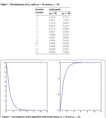
Table 1 The behavior ofxnwithx0= 10 andx0= –10

Iterative number

Initial point

x0= 10 x0= –10

1 3.3333 –3.5157

2 0.9411 –1.5857

3 0.2374 –0.6642

4 0.0556 –0.2619

5 0.0124 –0.0989

6 0.0027 –0.0362

7 0.0006 –0.0129

8 0.0001 –0.0045

9 0.0000 –0.0016

10 0.0000 –0.0005

11 0.0000 –0.0002

12 0.0000 –0.0001

13 0.0000 –0.0000

(22)

From Lemma ., we haveF(Tri) =GEP(,Ai) = . DeﬁneS:K→KbyS(x) =sin(x). Then

Sis nonexpansive andF(sin(x)) ={}. So, ={}. Assume thatI={, },A= ,{vn}={}, f(x) =x_,rn,i=₍_n_+)(n_i_+),αn=_n,βn=_andδn,i=_,Ci= ,i∈I. Hence,

⎧ ⎪ ⎪ ⎪ ⎪ ⎪ ⎨ ⎪ ⎪ ⎪ ⎪ ⎪ ⎩

un,=__n_+xn, un,=–__nn+_+xn, yn=–n

_+_n_–_n_– n_+_n_+_nxn, xn+=_xn+_sin(–n

_+_n_–_n_– n_+_n_+_nxn).

Then, by Theorem ., the sequence{xn}converges strongly to ∈ . Table  and Figure  indicate the behavior ofxnfor algorithm (.) withx=  andx= –. We have used

MATLAB withε= –.

Competing interests

The authors declare that they have no competing interests.

Authors’ contributions

All authors contributed equally, and they also read and ﬁnalized manuscript.

Received: 2 August 2016 Accepted: 12 September 2016

References

1. Blum, E, Oettli, W: From optimization and variational inequalities to equilibrium problems. Math. Stud.63, 123-145 (1994)

2. Combettes, PL, Histoaga, SA: Equilibrium programming using proximal like algorithms. Math. Program.78, 29-41 (1997)

3. Browder, FE, Petryshyn, WV: Construction of ﬁxed points on nonlinear mappings in Hilbert spaces. J. Math. Anal. Appl. 20, 197-228 (1967)

4. Acedo, GL, Xu, HK: Iterative methods for strict pseudo-contraction in Hilbert spaces. Nonlinear Anal.67, 2258-2271 (2007)

5. Rockafeller, RT: On maximality of sums of nonlinear operators. Trans. Am. Math. Soc.149, 75-88 (1970) 6. Cegielski, A: Iterative Methods for Fixed Point Problems in Hilbert Spaces. Springer, London (2011)

7. Ansari, QH, Schaible, S, Yao, JC: The system of generalized vector equilibrium problems with applications. J. Glob. Optim.22, 3-16 (2002)

8. Barbagallo, A: On the regularity of retarded equilibria in time-dependent traﬃc equilibrium problems. Nonlinear Anal.71, 2406-2417 (2009)

9. Barbagallo, A, Daniele, P, Maugeri, A: Variational formulation for a general dynamic ﬁnancial equilibrium problem: balance law and liability formula. Nonlinear Anal.75, 1104-1123 (2012)

10. Huang, NJ, Fang, YP: Strong vectorF-complementary problem and least element problem of feasible set. Nonlinear Anal.61, 901-918 (2005)

11. Cai, G, Bu, S: A viscosity scheme for mixed equilibrium problems, variational inequality problems and ﬁxed point problems. Math. Comput. Model.57, 1212-1226 (2013)

12. Chang, SS, Joseph Lee, HW, Chan, CK: A new method for solving equilibrium problem ﬁxed point problem and variational inequality problem with application to optimization. Nonlinear Anal.70, 3307-3319 (2009)

13. Liu, LS: Ishikawa and Mann iterative process with errors for nonlinear strongly accretive mappings in Banach space. J. Math. Anal. Appl.194, 114-125 (1995)

14. Peng, JW, Wu, SY, Yao, JC: A new iterative method for ﬁnding common solutions of a system of equilibrium problems, ﬁxed-point problems, and variational inequalities. Abstr. Appl. Anal. (2010). doi:10.1155/2010/428293

15. He, Z, Du, WS: Strong convergence theorems for equilibrium problems and ﬁxed point problems: a new iterative method, some comments and applications. Fixed Point Theory Appl. (2011). doi:10.1186/1687-1812-2011-33 16. Thianwan, S: Strong convergence theorems by hybrid methods for a ﬁnite family of nonexpansive mappings and

inverse-strongly monotone mappings. Nonlinear Anal. Hybrid Syst.3, 605-614 (2009)

17. Zhao, J, He, S: A new iterative method for equilibrium problems and ﬁxed point problems of inﬁnitely nonexpansive mappings and monotone mappings. Appl. Math. Comput.215, 670-680 (2009)

18. Takahashi, S, Takahashi, W: Strong convergence theorem for a generalized equilibrium problem and a nonexpansive mapping in a Hilbert space. Nonlinear Anal.69, 1025-1033 (2008)

19. Zhang, SS, Rao, RF, Huang, JL: Strong convergence theorem for a generalized equilibrium problem and ak-strict pseudocontraction in Hilbert spaces. Appl. Math. Mech.30(6), 685-694 (2009)

20. Shehu, Y: Iterative method for ﬁxed point problem, variational inequality and generalized mixed equilibrium problems with applications. J. Glob. Optim.52, 57-77 (2012)

21. Hao, Y, Cho, SY, Qin, X: Some weak convergence theorems for a family of asymptotically nonexpansive nonself mappings. Fixed Point Theory Appl.2010, Article ID 218573 (2010)

(23)

23. Scherzer, O: Convergence criteria of iterative methods based on Landweber iteration for solving nonlinear problems. J. Math. Anal. Appl.194, 911-933 (1991)