An Evaluation of Collective Mod of One-dimensional Fermi Gas in Weak and Strong Coupling Limit

(1)

An Evaluation of Collective Mod of One-dimensional Fermi

Gas in Weak and Strong Coupling Limit

PRADHAN DURGA SHANKAK PRASAD* and L. K. MISHRA

*Department of Physics, R. K. D. College Patna, Bihar, INDIA.

Department of Physics,

Magadh University, Bodh Gaya, Bihar, INDIA. (Received on: February 11, 2013)

ABSTRACT

Collective mode of one- dimensional Fermi gas has been evaluated over the whole coupling regime from weak coupling (high density) to strong coupling (low density).The evaluation has been performed using theoretical model of Alam and Schuck

taking attractive ߜ interaction potential under RPA approximation

at zero temperature. We observe that in the weak-coupling limit particle-hole RPA approaches to low momenta and the collective mode in the strong coupling limit reproduces the Bogoliubov mode for the weakly interacting bosons. Our theoretically evaluated results are in good agreement with other theoretical workers.

Keywords: collective mode, interaction potential, Random Phase

Approximation (RPA) Quasi-particle, weak- coupling, strong coupling, Bogoliubov mode.

INTRODUCTION

The one dimensional Fermi gas with attractive δ interaction among the fermions has been used as a model to know the physical properties of realistic Fermi system. The exact solution for its ground state energy is known from the Bathe ansatz1, therefore one can test approximate solutions of the systems. Quick, Esbagg and deLalno2

(2)

the exact solution in both weak and strong coupling. In this sense, the system may serve as a simple model to study the transition between weak and strong coupling superconductivity in 1D Fermi system. This transition between weak and strong coupling has been discovered by Leggett3 and by Noziers and Schmitt Rink4 in three dimensions. The simple form of the interaction allows one to carry out approximation beyond the mean-field level such as ordinary random phase approximation (RPA's) or generalized RPA's in controlled fashion. In this approximation, one is able to calculate contribution to the ground state energy of the system beyond the mean field ground state energy. Williams and Bloch5 have also discussed the ordinary (particle hole) RPA for the one dimensional electron gas. The same approach was also applied by Bernner and Haug6. Friesen and Bergersen7 have applied Singwi Sjolander generalization of RPA8 to the ID electron gas. This model can serve as an initial approximation to realistic systems such as quasi one dimensional metal9.

In this paper, using the theoretical formalism of T. Alm and P. Schuck10, we have studied the collective modes of the one dimensional Fermi gas within the quasi particle random phase approximation (RPA). One calculates the collective excitations for the 1D attractive Fermi gas with a δ interaction at T = 0 by applying the quasi particle RPA. One obtains quasi particle RPA equation for the two quasi particle propagator starting from the Bogoliubov transformed Hamiltonian of the system using the equation of motion for the two particle Green's function. The homogeneous two particle equation yields the condition for

the collective excitation in the system. It coincides with result found by Anderson11, Rickayzen12, Bardasis and Schrieffer13 and othersl4,15 by the equation of motion method. MATHEMATICAL FORMULAE USED IN THE STUDY

One writes the Hamiltonian for one dimensional Fermi gas in second quantization

H k C C k k V K K C C C C k

k k

k k k k

k k k k

=

∑

∈

b g

+ +1

∑

〈 〉 + +

4 1 2 3 41 2 3 4

1 2 3 4

| | , , ,

(1) where ki denote momentum and spin

quantum number of the particle and 〈k k V K K1 2| | 3 4〉 is the anti-symmetrized matrix element of the two body interaction. Using Bogoliubov transformation of the creation and annihilation operators Hamiltonian (1) is transformed into a new form. The transformed Hamiltonian is derived by several author, 16-18 The transformed Hamiltonian is written in the following form

H H H H H C

H H C

H o

k k k k k

k k k k k k k

k k k k k k k k k k k k

= + + +

+ +

+

+ + +

+ + + +

∑

1 2 1 1 2

2 1 2 1

1 2

1 2 3 4 1 3 4

1 2 3 4

1 2 3 4 1 3 4

1 2 3 4

1 2 3 4 1 3 4

1 2 3 4

11 20

2 40

2 31

2 22

2

1 2

1 4

α α α α

. .

d

i

d

i

d

i

(3)

the well known relations of BCS gap equation19.

The H31 term in the Hamiltonian in eqn (2) does not contribute to the RPA equations. The other terms H40 and H22 in the Hamiltonian describe the residual interaction among the quasi particle.

These terms are neglected in the model BCS approximation. Therefore in order to go beyond the BCS mean field approximation one has to include the residual interaction among the quasi particle. Now, one can treat the quasi particle within the generalized RPA approximation. For this, one introduces two particles Green's function with respect to quasi particle basis and derive the equation of motion for the Green's function G. The equation has the form of Dyson equation20 for the two particle propagator matrix G. The static elements of the mass operator A and B are given by the double commutation21

~

, ,

A A E E

A H

k k k k k k k k k k k k k k

k k k k k k j k k

1 2 3 4 1 2 3 4 1 2 1 2 3 4

1 2 3 4 1 2 3 3

= − +

= + +

d

i

δ δ

α α α α

(3) and

B

_{k k k k} _k _k

H

_k _k

1 2 3 4

= −

α α

2 1

,

α α

1 3

(4)

Here refers to averaging with respect to the BCS ground state. But in place of BCS ground state one has correlated ground state which corresponds to a generalized quasi particle RPA22.

Taking δ interaction one solves the system equation in the ω representation. One obtains coupling equation for G11 and G21 also for G22 and G21. One obtains

G

kq

E

G

kq

E

k q k q 0 11 0 22

1

,

, ,

ω

b

g

d

i

b

g

d

i

=

−

=

+

(5) where

E

_{k q}_,

=

E

_k

+

E

_{k q}₊

We have assumed that collective pairs have zero total spin One arrives on the expressions

G kk q G kk q G kq

E E m k q Z

E n k q k q

k k

k q

k q k q

k q k q k q

11 21 0 11 2 2 1 2 ′ + ′ = + − + + ′ ′ ′ ′ , , , ( , ) , , , , , , , , , ω ω ω δ ω ω ω ω ω

b

g

b

g

b

g

d

i

b

g

Λ l

b

g

Γ

(6) and

G kk q G kk q

G kq

E m k q Z

n k q E k q

k k

k q

k q k q

k q 11 21 0 11 2 2 1 2 ′ − ′ = + − + + ′ ′ ′ ′ , , , , , , , , , , , , ω ω ω δ ω ω ω ω ω ω

b

g

b

g

b

g

d

i

b

g

b

g

Λ l

b

g

Γ

(7) The quantities Z, Λ and Γ are given by the equations

Z_{k q} v m k q G k kq G k kq k

′

′′

= −

∑

′′ ′′ + ′′

,ω ,ω ,ω

2

11 21

b

g

b

g

b

g

(8a)

Λk q k

v n k q G k kq G k kq

, ,ω= − ′′, ′′ ,ω + ′′ ,ω

′′

∑

b

g

11

b

g

21

b

g

(8b)

Γk q k

v k q G k kq G k kq

, ,ω = − ′′, ′′ ,ω + ′′ ,ω

′′

∑

l

b

g

11

b

g

21

b

g

(8c) The quantities m(k,q), n(k,q) and l(k,q) are combination of uk and vk and is given by

(4)

n k q

b

,

g

=u uk k q+ +v vk k q+ _(9b)

l _{k q} _{u u} _{v v}

k k q k k q

,

b

g

= + − + _(9c)

and

u

v

E

k k k k 2 2

1

2

1

= −

=

L

+

N

M

O

Q

P

ε

(9d) Where

ε

µ

ε

k k k

HF

k k k

v

E

=∈ + −

= 2 +∆2

(9e)

Multiplying in equation (7) subsequently with m with n and in equation (7) with

l

and summing over k, one arrives at the system of equation for the quantities Z, Λ and Γ

(

)

(

)

(

)

(

)

(

)

(

)

(

)

(

)

(

)

, , , , , , , , , , , , , , , , , ,

1 , , ,

, 1 , 2 ,

, , 1 ,

2 2

E n n n E n m

n E m

E n m n E m m

vI q vI q vI q

v v

I q I q vI q

ω

ω ω

ω

ω ω ω

   ₊    +     +     l

l l l l

l

×

F

H

G

GG

I

K

J

JJ

=

−

F

H

G

I

K

J

Λ

Γ

Z

vn k q G

v k q G

v

m k q G

q l

l

, ,

,

ω

b

g

b

g

b

g

0 11 0 11 0 11

2

(10) The quantity Ia b c are in the notation

I a k q b k q c k q

E

a b c

k q k , , , , , , = −

∑

b

g b

g

d

ω

2 2

i

(11) Here a(k,q) = [Ek,qω] and b(k,q), c(k,q) =

[n(k,q),

l

(k,q), m(k,q)]. This is a linear in homogenous system of equation for the quantities Λ, Γ and Z. This can be solved

with the help of matrix inversion. Equation (10) is a eigen value problem for the determination of the collective modes in the quasi particle RPA. The condition for the nontrivial solution is the vanishing of determinant. ( ) ( ) ( ) ( ) ( ) ( ) ( ) ( ) ( ) , , , , , , , , , , , , , , , , , ,

1 , , ,

, 1 , 2 , 0

2 , 2 , 1 ,

E n n n E n m

n E m

E n m n E m m

vI q vI q vI q

v I q v I q vI q

Ω

Ω Ω

Ω

+ Ω Ω Ω

Ω + Ω Ω =

Ω Ω + Ω

l

l l l l

l

(12) where Ω (q) denotes the eigen value for the collective excitation.

Weak coupling case

The analysis of the weak coupling case has been given by Belkker and Randeria23. One quotes their result for the weak coupling collective made in one dimension.

Ω

q

v

m

k

m

q

F F

b g

= −

L

N

M

O

Q

P

1

1 2

π

₍₁₃₎

where the density of states in one dimension for parabolic dispersion was used. The long wavelength collective modes in the weak coupling case have a phonon like spectrum and are independent of the gap. If one compares equation (13) with the small-q expansion of the collective modes in the particle hole RPA, one finds that both coincides. This means that in weak coupling the behavior of collective modes for small q is not changed from the normal particle hole RPA.

However, for large q and in particular near the point q=2kF the

(5)

Strong coupling limit

Now, from equation (12) one can expand the determinant of the collective modes for small -q and - Ω limit with respect to small gap. In the strong coupling limit the gap goes to zero with density.2 One expands the gap equation in terms of ∆2

1

2

1

0 2

2 1 2

=

+

F

H

G

I

K

J

∞

z

v

dk

k

π

ξ

∆

= v

z

∞dk −v

z

∞dk = v J −v J

k k

2

1 4

1

2 4

0

2 0

3 1

2 3

π ξ π ξ π π

∆ ∆

(14) Here one has introduced integral Ji. It has

been evaluated for the strong coupling limit i.e. for µ*<O. Here µ * is effective chemical potential including the quasi particle shift

J dk

k m

i = = i

+

F

HG

I

KJ

∞

z

1

2

2 0

µ

*

(15a)

J dk k

k m

i2 i

2

2 0

2

= =

+

F

HG

I

KJ

∞

z

µ

*

(15b) Then

J m

1

1 2 1 2

2

1 2 3 2

3

1 2 7 2 5 2

2

3 2

=

= =

π

µ

π

µ

π

µ

/

*

e

j

e

j

e

j

_(15c)

Now in equation (14) the integral in the first line is convergent for a contact interaction without a cutoff due to the one dimensionality of the system. An analogous expansion of the BCS density equation yields

n= 1 J

2

2 2

π

Λ (16)

Now, the effective chemical potential can be expressed in terms of the density and the coupling strength as

µ

*

b

g

1 2

2

1 2 2

8

2

64

3

8

=

m v

±

mv

−

nv

(17) In the limit of zero density or zero gap, respectively equation (17) yields the condition

2

4

2

0

µ

*

=

mv

=

E

(18)

This shows that in the extreme strong coupling limit the chemical potential i.e. the energy to remove a particle from the system in just half the two particle binding energy -EO in the Vacuum.

2

The long wavelength dispersion relation in the strong coupling limit is given by

Ω

b g

q

=

cq

(6)

Ω

q

vn

m

q

b g

=

L

NM

O

QP

4

1 2

(19b) Introducing the pair mass mB = 2m and the

pair density nB = n/2 the above expression

reduces to

Ω

q

vn

m

q

B

b g

=

L

NM

O

QP

4

1 2

(19c) Equation 19(c) is the well known Bogoliubov dispersion relation for the weakly interacting Bose gas24,25 in the limit of small q which is linear in q i.e. phonon like. Thus starting from interacting fermions with an attractive interaction the quasi particle RPA in the strong coupling limit yields the dispersion relation for weakly interesting gas of bosons (two particle bound states). The magnitude of the repulsive interaction among the bosons in equation 19(c) is given by the fermionic interaction strength v and is consistent with the result of Hanssmann26 and others.27-32

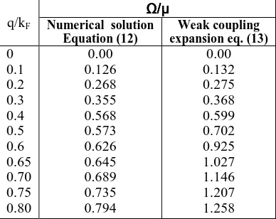
Table T1

An Evauated results of collective mode Ω for small momenta q in the weak coupling limit

(µ*=3.386 E0) The numerical solution is

compared with weak coupling expansion (13).

q/kF

Ω/µ Ω/µΩ/µ Ω/µ

Numerical solution Equation (12)

Weak coupling expansion eq. (13)

0 0.1 0.2 0.3 0.4 0.5 0.6 0.65 0.70 0.75 0.80

0.00 0.126 0.268 0.355 0.568 0.573 0.626 0.645 0.689 0.735 0.794

0.00 0.132 0.275 0.368 0.599 0.702 0.925 1.027 1.146 1.207 1.258

DISCUSSION OF RESULTS

In this paper, using the theoretical formalism of T. Alm and P. Schuck,10 we have studied the behavior of collective modes over the coupling regime weak coupling (high density) to strong coupling (low density). We observe that the treatment of the residual interaction in the Hamiltonian (2) within the quasi particle or generalized RPA allows one to study the behavior of the collective over the whole coupling range. Collective modes in one dimension were found for the case of an attractive δ interaction. One observes that in the weak coupling limit one recovers Anderson's results11 whereas in the strong coupling limit the Bogoliubov dispersion relation24 for the interacting Bose gas of two particle pairs can be derived from the quasi particle RPA. This is consistent with the fact that the BCS theory is capable of describing the extreme strong coupling limit i.e. the gas of two particle bound state properly and reproduces the exact result for the ground state energy in this limit.2 In table Tl' we have presented

for small momenta q in the weak coupling limit (µ*=3.386Eo). The numerical solution

equation (12) is compared with weak coupling expansion equation (13). Both solution coincides at q/kF = 0.4. This shows the consistency of the numerical solution with the well known weak coupling result which was obtained by Anderson11 in the 3D case. In table T2, we have presented the

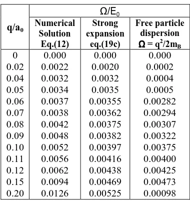
evaluated results of collective mode Ω for small momentum q in the strong coupling case (µ* = (-) 0.4966 E0)' The numerical

(7)

=q2/2mB. We observe that the numerical

solution starts linearly in q and is consistent with the strong coupling expansion gives in equation 19(c). This confirms the interpretation of the collective excitations in the strong coupling limit as Bogoliubov sound modes of the two particle Bose gas that is formed in the limit. The free particle solution reached the full solution for large q. Some recent33-37 calculations also reveal the same type of behavior.

Table T2

An Evauated results of collective mode Ω for small momenta q in the strong coupling limit

(µ*=(-)0.4966 E0) The numerical solution

[eq.(12)] is compared to the strong coupling expansion [eq.(19c)] and free particle dispersion

Ω =q2/2mB(a0 =Bohr radius)

q/a0

Ω/Ε0

Numerical Solution

Eq.(12)

Strong expansion

eq.(19c)

Free particle dispersion

Ω ΩΩ Ω = q2_/2m

B

0 0.02 0.04 0.05 0.06 0.07 0.08 0.09 0.10 0.11 0.12 0.15 0.20

0.000 0.0022 0.0032 0.0034 0.0037 0.0038 0.0042 0.0048 0.0052 0.0056 0.0062 0.0094 0.0126

0.000 0.0020 0.0032 0.0035 0.00355 0.00362 0.00375 0.00382 0.00397 0.00416 0.00438 0.00469 0.00525

0.000 0.0002 0.0004 0.0005 0.00282 0.00294 0.00307 0.00322 0.00375 0.00400 0.00425 0.00473 0.00098

REFERENCES

1. M. Gaudui, Phys. Lett. B 24, 55 (1967). 2. R.M. Quick, C. Esebagg and M. de

Llano, Phys. Rev. B 47, 11512 (1993).

3. A.J. Leggett, J. Phys. (Phys) Calling 41, C7-19 (1980).

4. P.Nozieres and S. Schmitt - Rink, J. Low. Temp. Phys. 59, 195 (1985). 5. P.F. Williams and A.N. Bloch, Phys.

Rev. B 10, 1097 (1974).

6. S. Brenuer and H. Haug, Z. Phys. B 84,81 (1991).

7. W.I. Friesen and B. Bergersen, J. Phys. 13, 6627 (1980).

8. R. Cote and A. Griffin, Phys. Rev. B 48, 10404 (1993).

9. Chemistry and Physics of One-Dimensional Metals, Vol. 25 of NATO, Advanced Study Institute, Series B : Physics edited by 1. Keller (Plenum, New York, 1971).

10. T. Alm and P. Schuck, Phys. Rev. B 54, 2471 (1995).

11. P. Anderson, Phys. Rev. 112, 1901 (1958). 12. G. Rickayzen, Phys. Rev. 115,795 (1959). 13. A. Bardasis and J.A. Schrieffer, Phys.

Rev. 121, 1050 (1961).

14. Y.A. Bychkov, L.P. Gorkov and I. E.dzyaloshinui, Sov. Phys. JETP 23, 489 (1966).

15. R.E. Peierls, Quantum Theory of Solid (Oxford University Press, New York, 1955). 16. G. Fano, Nuovo Cimento 6, 959 (1960).

17. D.H. Kobe and W.B. Cheston, Ann. Phys. (N.Y.) 20, 279 (1962).

18. P. Ring and P. Schuck, The Nuclear Many Body Problem, Springer, Berlin, (1980).

19. T. Kostyrko and R. Mienas, Phys. Rev. B 46, 1025 (1992).

20. J.O. Sofo, C.A. Balseiro and H.E. Castillo, Phys. Rev. B 45, 9860 (1992). 21. P. Schuck and S. Ethofer, Nucl. Phys. A

(8)

22. J. Dukelsky and P. Schuck, Nucl. Phys. A 512,466 (1990).

23. L. Belkhir and M. Randeria, Phys. Rev. B 49, 6829 (1994).

24. N.N. Bogoliubov, J. Phys. (Moscow) 11,23 (1947).

25. A.L. Fetter and J.D. Walecka, Quantum Theory of Many Particle System (McGraw Hill, New York, 1971). 26. R. Haussmann, Z. Phys. B 91,291

(1993).

27. G. Ropka, Ann. Phys. (Leipzig) 3, 145 (1994).

28. P. Krugerand and P. Schuck, Europhys. Lett. 27, 395 (1994).

29. A.S. Alexandrow and S.G. Ruskin, Phys. Rev. B 47, 5141 (1993).

30. D.V. Khrebhchenko, Nucl. Phys. B 643,

515 (2002).

31. D.A. Ivanov, Phys. Rev. B 70, 104503 (2004).

32. M. Hermele, T.Senthil and Matthew P.F. Fisher, Phys. Rev. B 72, 104404 (2005). 33. M. M. Parish, F. M. Marchetti, A.

Lamacraft and B. D. Simons, Nature Phys. 3, 124 (2007).

34. J. T. Stewart, J. P. Gaebeler and D. S. Jin, Nature (London) 454,744 (2008). 35. M. Sato, Y. Takahashi and S. Fujimoto,

Phys. Rev. Lett. (PRL) 103, 020401 (2009).

36. M.Z. Hasan and C. L. Krane, Rev. Mod. Phys.82, 3045 (2010).