R E S E A R C H
Open Access
On increasing the convergence rate of
difference solution to the third boundary
value problem of elasticity theory
Givi Berikelashvili
1*and Bidzina Midodashvili
2*Correspondence:
[email protected] 1A. Razmadze Mathematical
Institute, I. Javakhishvili Tbilisi State University, Tbilisi, 0177, Georgia Full list of author information is available at the end of the article
Abstract
We consider the third boundary value problem of static elasticity theory (stiff contact problem) in a rectangle, for solution of which we use a difference scheme of
second-order accuracy. Using this approximate solution, we correct the right-hand side of the difference scheme. It is shown that the solution of the corrected scheme is convergent at the rateO(|h|m) in the discreteL
2-norm, provided that the solution of the original problem belongs to the Sobolev space with exponentm∈[2, 4].
MSC: 65N06; 74G15
Keywords: difference scheme; method of corrections; improvement of accuracy; elasticity
1 Introduction
The problem of accuracy is the main problem in the theory of difference schemes as well as in applications. One approach for obtaining solutions with improved accuracy is rep-resented by the idea of refinement by differences of higher order, which was offered by Fox []: the right-hand side of the difference scheme is corrected by the solution obtained on the first stage and the scheme is repeatedly solved on the same grid. This empirical idea is simple, although its theoretical foundation encounters essential difficulties. This is shown by Volkov’s papers [–], where the above-mentioned method was founded only for the Poisson and Laplace equations, besides, the input data in the problems were chosen so as to ensure that the exact solution belongs to the Hölder classC,λ(¯).
In the development of the mentioned method there are two possible difficulties. The first one consists of finding the correcting addend, and the second is related to obtaining ana prioriestimate of convergence. To overcome these difficulties we use the method for derivation of estimates for the convergence rate of difference schemes developed in the last years by Samarskii and other authors (e.g., see [–]), in which the convergence rate is compatible with the smoothness of the solution of the original differential problem. For elliptic problems, such estimates have the form
U–uWs(ω)≤c|h| m–su
Wm(), m>s≥, ()
whereuis the solution of the original differential problem,Uis an approximate solution,
sandmare integer and real numbers, respectively, and · Ws(ω) and · Ws() are the
Sobolev norms on the sets of functions of discrete and continuous arguments, respectively. Hereafter bycwe denote positive constants that are independent of|h|anduand can be distinct in distinct formulas.
For obtaining a difference solution of the Dirichlet problem posed for elliptic equations, in [, ] was considered the aforementioned method of correction.
In [, ] is considered the third boundary value problem of static elasticity theory (stiff contact problem) in a rectangle. For corresponding difference schemes, when s= , , and <m–s≤, there are accepted estimates of type ().
In the present paper, for the same problem, we construct a correction term for the right-hand side of the difference scheme. It is proved that the corrected scheme converges at the rateO(|h|m) in the discreteL
(ω)-norm provided that the exact solution belongs to
the Sobolev spaceWm
(),m∈[, ].
2 Statement of the problem
Below, everywhere we assume that indexα= , andβ= –α.
Let¯ ={x= (x,x) : ≤xα≤lα}represent a rectangle with boundary.
Consider the problem
(λ+ μ)∂
u
∂x
+ (λ+μ) ∂
u
∂x∂x
+μ∂
u
∂x
+f(x) = ,
μ∂
u
∂x
+ (λ+μ) ∂
u
∂x∂x
+ (λ+ μ)∂
u
∂x
+f(x) = , x∈,
()
uα(x) = , ∂u
β(x)
∂xα = , x∈,xα= ,lα. ()
Hereλ,μ= const,μ> .λ≥–μare Lamé coefficients, u = (u,u)T is an unknown dis-placement vector, and f = (f,f)Tis the given vector.
As usual, by the symbolWs
(),s≥, we denote the Sobolev space. For integersthe
norm inWs
() is given by the formula uWs
()= s
j= |u|
Wj(), |u|
Wj()=
|ν|=j
DνuL (),
whereDν=∂|ν|/(∂xν
∂x
ν
), andν= (ν,ν) is a multi-index with non-negative integer
com-ponents,|ν|=ν+ν.
Ifs=¯s+ε, where¯sis an integer part ofsand <ε< , then
uWs
()=u
W¯s()+|u|
Ws(),
where
|u|Ws()=
|ν|=s¯
|Dνu(x) –Dνu(y)| |x–y|+ε dx dy.
Particularly, fors= we haveW =L.
Let us introduce the mesh domains
¯
ωα={xα=iαhα:iα= , , . . . ,nα,nαhα=lα,nα≥},
ωα=ω¯α\ {,lα}, ω+α=ωα∪ {lα},
γ–α=
x= (x,x) :xα= ,xβ∈ωβ
, γ+α=
x= (x,x) :xα=lα,xβ∈ωβ
,
γβ=γ\(γ–α∪γ+α), ω=ω×ω, ω¯=ω¯× ¯ω,
ω+=ω+×ω+, γ =ω¯\ω,
¯ γ±α=
x= (x,x)∈γ:xα= (lα±lα)/
, ω()=ω× ¯ω, ω()=ω¯×ω, |h|=h+h,α=hαwhenxα∈ωα,α=hα/ whenxα= ,lα.
Further, we define difference quotients in thexαdirection as follows:
Vxα=
V(+α)–V/hα, Vx¯α=
V–V(–α)/hα, V◦
xα= (Vxα+Vx¯α)/,
where
V(±)(x) =V(x
±h,x), V(±)(x) =V(x,x±h).
The notationsV(±.α)will have a similar meaning. Let
IαV(x) :=V(x) +V
(–α)(x)
. Denote
ααV:=
⎧ ⎪ ⎨ ⎪ ⎩
hαVxα, x∈γ–α,
Vx¯αxα, x∈ ¯ω\γα,
–h
αVx¯α, x∈γ+α,
V:=
⎧ ⎪ ⎨ ⎪ ⎩
Vxα◦
xβ, x∈γ–α,
V◦
xx◦, x∈ω, Vx¯
α◦xβ, x∈γ+α.
On the set of mesh functions we define scalar products and norms: (Y,V)ω˜ =
x∈ ˜ω
hhY(x)V(x), Yω˜= (Y,Y)/ω˜ , ω˜⊆ ¯ω,
(Y,V)(α)=
x∈ω(α)
hαβY(x)V(x), Y(α)= (Y,Y)/(α).
ByHh◦ (ω) we denote a set of two-dimensional vector-functions V = (V,V)T, whose
components are defined onω¯ and equal to zero onγα, respectively. LetHhbe the set of
two-dimensional vector-functions, whose components are defined on the meshesω(α),
respectively.
Define inH◦h(ω) the inner product and the norms:
(U, V) =U,V()+U,V(), U= (U, U)/,
U W(ω):=
α=
Uα
(α)+U
α
(α)+ U
α
¯
xx¯
ω+
For functions, defined on, we need the following averaging operators:
S–u(x) :=
h
x
x–h
u(t,x)dt, Tu(x) :=
h
x+h
x–h
h–|x–t|
u(t,x)dt,
Tu(,x) :=
h
h
(h–t)u(t,x)dt,
Tu(l,x) :=
h
l
l–h
(h–l+t)u(t,x)dt.
Analogously are defined operatorsT,S–. Note that these operators are commutative and
Tα∂
u
∂x
α
=ux¯αxα, Tα
∂u
∂xα =
S–αux
α.
3 Difference scheme, correction procedure, and main result
At thefirst stage, we approximate problem (), () by the difference scheme
(λ+ μ)U+ (λ+μ)U+μU+F= , x∈ω(),
μU+ (λ+μ)U+ (λ+ μ)U+F= , x∈ω(), ()
Uα(x) = , x∈γα, Fα(x) =TTfα.
Let us rewrite the difference scheme () in the operator form
LhU= F, U∈ ◦
Hh, F∈Hh, ()
where
Lh= –
(λ+ μ)+μ (λ+μ)
(λ+μ) μ+ (λ+ μ)
,
U=U,UT, F=F,FT.
Lemma [] The operatorLh: ◦
Hh→Hhis self-adjoint,positive definite,and the estimate
LhV ≥μVW
(ω) ()
is valid.
Due to the positive definiteness of Lh the solution of equation () (or the difference
scheme ()) exists and is unique. The rate of convergence of the scheme () is determined by the estimate []
U– uW
(ω)≤c|h| m–u
Wm
To construct and study a corrector, we use the operators
PαV:=
⎧ ⎪ ⎨ ⎪ ⎩
Iβ(V¯x
α◦xα), xα∈ωα\ {hα},
Iβ(V¯xαxα–
hα
Vx¯αxαxα), xα=hα,xβ∈ω +
β, Iβ(V¯xαx¯α+
hα
Vx¯αx¯αx¯α), xα=lα, BV:=
⎧ ⎪ ⎨ ⎪ ⎩
hαV (+α)
xβ , x∈γ–α,
Vxx, x∈ω,
–
hαVxβ, x∈γ+α, DαV:=
⎧ ⎪ ⎨ ⎪ ⎩
Vx¯αxα, x∈ω(α),
Vxαxα– hα
Vxαxαxα, x∈ ¯γ–α,
Vx¯αx¯α+ hα
Vx¯αx¯αx¯α, x∈ ¯γ+α.
At thesecond stage, we use the earlier-found solution of the difference scheme () for defining the correction termRUand on the same grid solve the difference scheme
LhU˜ = F +RU, U˜ ∈ ◦
Hh, F∈Hh, ()
where
R:=
(λ+ μ)hD+μhD –(λ+μ)(h
BP+
h
BP)
–(λ+μ)(h
BP+
h
BP) (λ+ μ)
h
D+μ
h
D
.
The following theorem is the main result of the present paper.
Theorem Let the solution of problem(), ()belong to the space Wm(),m≥.Then the convergence rate of the corrected difference scheme()in the discrete L-norm is given
by the estimate
˜U– uL(ω)≤c|h| mu
Wm
(), ≤m≤. ()
4 A priori estimate for the error of the corrected solution
Let
ζααα :=Tβuα–uα–h
β
Dβu
α, x∈ ¯ω, ()
ζααβ :=Tβuβ–uβ–h
β
Dβu
β, x∈ω
(β), ()
ζα :=SSuα–IIuα+
h
Pu
α
+h
Pu
α
, x∈ω+. ()
ByZ˜= u –U˜ we denote the error in the solution of the corrected difference scheme ().
Lemma The errorZ˜ is a solution of the problem
whereZ= u – Uis the error in the solution of the scheme()and
= (λ+ μ)
ζ
ζ
+μ ζ
ζ
+ (λ+μ)
B
B
ζ ζ
.
Proof From equalities (), () we have
TT
∂uα
∂x
α
=ααuα+h
β
αα
Dβuα+ααζααα, x∈ω(α), ()
TT
∂uβ
∂x
α
=ααuβ+h
β
αα
Dβuβ+ααζααβ , x∈ω(β). ()
It is not hard to verify that
TT
∂uα
∂x∂x
=B
S–S–uα, x∈ω(β). ()
Besides,
B
IIuα
=uα. ()
Indeed, in the casex= we have
B
IIu
=
h
IIu
(+) x =
h
Iu
(+) ◦ x =
h
(u)(+)+u
◦ x = h
(u)(+)–u
◦ x
=u◦
xx=u
.
It is easy to verify also the other cases of (). As a result from () we obtain
TT
∂uα
∂x∂x
=uα–
h
BPu
α
–h
BPu
α
+Bζα, x∈ω(β). ()
Let us apply the operatorTTon the equations of system () on the grid pointsω(),ω(),
respectively, and then use equations (), (), (). The obtained results may be compactly written as follows:
Lhu= F +Ru+. ()
Subtracting () from equality () we obtain the required equality ().
Theorem For the solution of problem()the following a priori estimate is valid:
˜ZL(ω)≤c
|h|ZW (ω)+
α=
ζα
(α)+ζ
α
(α)+ζ
α
ω+
Proof First, note that based on the inequalities
L–h
αα
λββ
≤
μ,
L–h
B
B
≤
μ,
implied by (), we have
L–
h ≤c
α=
ζα(α)+ζα(α)+ζαω+
. ()
Further, the operatorLhis positive definite and self-adjoint, therefore,
L–
h RZ= sup
V=
|(RZ, V)|
LhV
. ()
Using the equalities obtained by partial summation,
⎧ ⎪ ⎪ ⎪ ⎨ ⎪ ⎪ ⎪ ⎩
(ααDβZα,Vα)(α)= (DβZα,ααVα)(α), sinceZα,Vα= forx∈γα,
(ββDαZα,Vα)(α)= (DαZα,ββVα)(α), by definition ofββ,
(BPαZβ,Vα)
(α)= (PαZβ,Vx¯αx¯)ω+, sinceV
α= forx∈γ α,
(BPβZβ,Vα)
(α)= (PβZβ,Vx¯α¯x)ω+, sinceV
α= forx∈γ α
and after considering the Cauchy-Schwarz inequality, for an estimate of the numerator of () we have
(RZ, V)≤c|h|ZVW
(ω). ()
Taking into account (), () from () we obtain
L–
h RZ≤c|h|ZW(ω). ()
Inequalities () and () together with
˜Z ≤L–h RZ+L–h
complete the proof of Theorem .
5 Proof of Theorem 1
To determine the rate of convergence of the corrected finite difference scheme () with the help of Theorem , it is sufficient to estimate the norms ofζα,ζα,ζα on the right-hand part of (). To this aim, we need the next lemma.
Lemma Let the linear functional l(u)be bounded in Wk(E),where k=k¯+,k is an¯ integer number, <≤.If l(u)equals zero on polynomials of two variables with order equal tok¯,then there exists a constant c,dependent on E,but not dependent on u(x),such that|l(u)| ≤c|u|Wk
This lemma is a particular case of the Dupont-Scott approximation theorem [], and it represents a generalization of the Bramble-Hilbert lemma [] (see,e.g., []).
Lemma Letu∈Wm
(),m∈[, ].Then for the expressions defined by equations(),
(), ()the following inequalities hold:
ζααα
(α)≤c|h|
muα
Wm(), ()
ζααβ (β)≤c|h|muβWm
(), ()
ζαω+≤c|h|muαWm
(). ()
Proof Let us denote byπthe set of third degree polynomials. In the casesx∈γ±β, taking
into account boundary condition, let us represent the valuesζααα in the form
ζααα =ζααα ±hβ
∂uα
∂xβ.
Particularly,
ζ =Tu–u–
h
∂u
∂x
–h
u
xx+ h
u
xxx, x∈γ–.
Lete={ξ= (ξ,ξ) :|ξ–x| ≤h, ≤ξ≤h}. Byu¯(t) we denote a function obtained
fromu(ξ) by changing the variablesξ
α+tαhα, and mapping the domaineontoE={t=
(t,t) :|t| ≤, ≤t≤}. Sinceu(ξ) =u(x+th,x+th) =u¯(t), the expressionζ
turns into
ζ =
( –t)u¯(,t)dt–u¯(, ) –
∂u¯(, )
∂x
–
¯
u(, ) – u¯(, ) +u¯(, )+
¯
u(, ) – u¯(, ) + u¯(, ) –u¯(, ).
Consequently,|ζ| ≤c¯uC(E)≤c¯uWm
(E) asW m
⊂Cwhenm> . Utilizing the fact
that ζ, as a functional of u¯, vanishes onπ (which can be verified directly) and using
Lemma , we obtain|ζ| ≤c|¯u|Wm
(E),m∈(, ]. Reverting to the old variables, this yields
ζ≤c|h|m(hh)–/uWm
(e), m∈(, ]. ()
In the casex∈γ+the estimate can be obtained analogously.
Whenx∈ω, we haveζ
=Tu–u– (h/)ux¯x. In this case the elementary domain e={ξ= (ξ,ξ) :|ξα–xα| ≤hα}, and we again obtain the estimate of the form () (see,e.g.,
[]). Consequently, we have
ζ
()=
ω()
hζ
≤c|h|m ω()
uWm
(e)≤c|h|
mu
Wm().
The caseα= in () can be proved in the same way.
Using the Taylor expansion we can show that
S–S–u–IIu= –
h
∂u
∂x
+h
∂u
∂x
(–.,–.)
foru∈π. ()
On the other hand, each of the following expressions:
ux¯α◦
xα, ux¯αxα–
hα
ux¯αxαxα, and ux¯αx¯α+
hα
ux¯αx¯αx¯α
equals ∂u(–.α)
∂xα foru∈π. Therefore, Pαu=Iβ∂
u(–.α)
∂x
α
=∂
u(–.,–.)
∂x
α
whenu∈π. ()
From (), () it is easy to see that the expressionsζα, as linear functionals with respect touα, turn into zero on the polynomials of third order and are bounded whenuα∈Wm
(),
m≥. Therefore, for them we have again the estimates similar to (), whence follows the validity of ().
Lemma is proved.
In view of () and the inequality (), taking into account the Lemma , the validity of Theorem is obvious.
6 Numerical experiments
Now, we present some numerical results to demonstrate the convergence order of the pro-posed method. The experimental order of convergence in the discreteL-norm is
com-puted by the formula
Ord(Y) =log Yh–u Yh/–u
,
where uis the exact solution of original problem, whileYh denotes the solution of the
difference scheme on the grid with steph.
Below, the symbolsU,U˜ denote solutions of the difference schemes (), (), respectively.
Example Consider the problem (), (), wherel,l= ,λ= ,μ= , and
f(x) = csin(πx)cos(πx), f(x) = ccos(πx)sin(πx), c=π(λ+ μ).
For calculation of the right-hand side of the difference scheme note that
Tαsin(πxα)=csin(πxα), Tαcos(πxα)=ccos(πxα), c=
πhsin
πh
. Therefore,
Fα=TTfα=cf
α
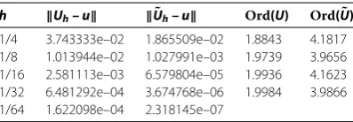
Table 1 Experimental order of convergence
h Uh– u ˜Uh– u Ord(U) Ord(U)˜
1/4 3.743333e–02 1.865509e–02 1.8843 4.1817 1/8 1.013944e–02 1.027991e–03 1.9739 3.9656 1/16 2.581113e–03 6.579804e–05 1.9936 4.1623 1/32 6.481292e–04 3.674768e–06 1.9984 3.9866 1/64 1.622098e–04 2.318145e–07
To solve the difference schemesLhY=ϕwe use the iterative method of minimal resid-uals
Y(k+)–Y(k)
τk
+LhY(k)=ϕ, k= , , , . . . ,∀Y()∈Hh◦ ,
where
τk=
(LhRes(k),Res(k))
(LhRes(k),LhRes(k))
, Res(k)=LhY(k)–ϕ.
It is clear that the exact solution
u(x) = sin(πx)cos(πx), u(x) = cos(πx)sin(πx)
belongs toW
(), therefore, for the refined scheme the fourth order of convergence is
expected.
The results of the calculations are given by Table .
Competing interests
The authors declare that they have no competing interests.
Authors’ contributions
All authors read and approved the final manuscript.
Author details
1A. Razmadze Mathematical Institute, I. Javakhishvili Tbilisi State University, Tbilisi, 0177, Georgia.2Faculty of Exact and
Natural Sciences, I. Javakhishvili Tbilisi State University, Tbilisi, 0186, Georgia.
Acknowledgements
This work was supported by the Shota Rustaveli National Science Foundation (Grant FR/406/5-106/12). The authors sincerely thank the referees for their helpful comments.
Received: 14 April 2015 Accepted: 19 November 2015 References
1. Fox, L: Some improvements in the use of relaxation methods for the solution of ordinary and partial differential equations. Proc. R. Soc. Lond. Ser. A190, 31-59 (1947)
2. Volkov, EA: On a method of increasing the accuracy of the method of grids. Dokl. Akad. Nauk SSSR96, 685-688 (1954) 3. Volkov, EA: Solving the Dirichlet problem by a method of corrections with higher order differences, I. Differ. Uravn.
1(7), 946-960 (1965)
4. Volkov, EA: Solving the Dirichlet problem by a method of corrections with higher order differences, II. Differ. Uravn.
1(8), 1070-1084 (1965)
5. Volkov, EA: A two-stage difference method for solving the Dirichlet problem for the Laplace equation on a rectangular parallelepiped. Comput. Math. Math. Phys.49(3), 496-501 (2009)
6. Lazarov, RD, Makarov, VL, Samarskii, AA: Application of exact difference schemes to the construction and study of difference schemes for generalized solutions. Math. USSR Sb.45(4), 461-471 (1983)
7. Lazarov, RD, Makarov, VL, Weinelt, W: On the convergence of difference schemes for the approximation of solutions of elliptic equations with mixed derivatives. Numer. Math.44(2), 223-232 (1984)
9. Jovanovi´c, BS, Süli, E: Elliptic boundary-value problems. In: Analysis of Finite Difference Schemes, pp. 91-243. Springer, London (2014)
10. Berikelashvili, G: Construction and analysis of difference schemes for some elliptic problems, and consistent estimates of the rate of convergence. Mem. Differ. Equ. Math. Phys.38, 1-131 (2006)
11. Berikelashvili, GK, Midodashvili, BG: Compatible convergence estimates in the method of refinement by higher-order differences. Differ. Equ.51(1), 107-115 (2015)
12. Berikelashvili, G, Midodashvili, B: Method of corrections by higher order differences for elliptic equations with variable coefficients. Georgian Math. J.23(2016, to appear)
13. Berikelashvili, GK: The convergence of the difference solution to the third boundary value problem of elasticity theory. Comput. Math. Math. Phys.38(2), 300-304 (1998)
14. Berikelashvili, GK: On convergence of difference schemes for the third boundary value problem of elasticity theory. Comput. Math. Math. Phys.41(8), 1182-1189 (2001)
15. Dupont, T, Scott, R: Polynomial approximation of functions in Sobolev spaces. Math. Comput.34(150), 441-463 (1987) 16. Bramble, JH, Hilbert, SR: Bounds for a class of linear functionals with application to Hermite interpolation. Numer.
Math.16(4), 362-369 (1971)