PhD Programme in Mathematics Department of Mathematics
Intrinsic differentiability and Intrinsic
Regular Surfaces in Carnot groups
Advisor:
Raul Serapioni
PhD Student:
Daniela Di Donato
Doctoral thesis in Mathematics, XXIX cycle
Department of Mathematics, University of Trento
Academic year 2016/2017
Supervisor: Raul Serapioni,University of Trento
University of Trento Trento, Italy
Ai miei genitori Tiziana e Franco, e a mio fratello Pier Paolo, per il loro sostegno.
1 Carnot groups 16
1.1 Carnot Carath´eodory spaces . . . 17
1.1.1 Vector fields on RN . . . . 17
1.1.2 Carnot Carath´eodory distance . . . 18
1.2 Lie groups and Lie algebras . . . 21
1.2.1 Homomorphisms and isomorphisms . . . 23
1.2.2 Exponential map . . . 24
1.2.3 The Baker-Campbell-Hausdorff formula . . . 27
1.2.4 Nilpotent groups . . . 28
1.3 Carnot groups of step κ . . . 29
1.3.1 Uniqueness of stratifications . . . 30
1.3.2 The dilation structure . . . 31
1.3.3 The Composition Law of G . . . 33
1.3.4 Left invariant vector fields . . . 41
1.3.5 Metrics on Carnot groups . . . 42
1.3.6 Hausdorff measures in a metric space: Application to Carnot groups . 45 1.3.7 Sum of Carnot Groups . . . 48
1.4 Groups of class B . . . 49
1.4.1 Characterization of Carnot groups of Step 2 . . . 49
1.4.2 Groups of class B . . . 53
1.4.3 Example: Free Step 2 Groups . . . 54
1.4.4 Example: H-Type Groups . . . 56
1.4.5 Example: H-groups in the Sense of M´etivier . . . 58
2 Differential calculus within Carnot groups 62 2.1 Complementary subgroups . . . 64
2.2 H-linear maps . . . 69
2.2.1 H-epimorphisms and H-monomorphisms . . . 71
2.2.2 H-quotients and H-embeddings . . . 73
2.3.1 P-differentiability . . . 74
2.3.2 C1G functions . . . 75
2.3.3 BVG functions . . . 84
2.4 G-regular surfaces . . . 86
2.4.1 (G(1),G(2))-regular surfaces . . . 86
2.4.2 G-regular surfaces . . . 88
2.5 Intrinsic graphs . . . 90
2.5.1 Intrinsic Lipschitz graphs . . . 94
2.5.2 Intrinsic difference quotients . . . 99
2.6 Intrinsic differentiability . . . 101
2.6.1 Intrinsic linear functions . . . 101
2.6.2 Intrinsic differentiability and graph distance . . . 104
2.6.3 Uniformly Intrinsic differentiability . . . 108
3 Intrinsic Regular Surfaces in Carnot groups 113 3.1 An characterization of G-regular surfaces . . . 115
3.2 1-Codimensional Intrinsic graphs . . . 119
3.2.1 The intrinsic gradient . . . 119
3.2.2 Broad∗ solutions and Dψ-exponential maps . . . 124
b compactly contained
⊕ direct sum of vector spaces
◦ composition of functions RN N-dimensional Euclidean space
∂xif partial derivative of the function f with respect to xi
LN Lebesgue measure in
RN
G a Carnot group
Hk k-th Heisenberg group
g Lie algebra of G
dcc Carnot-Carath´eodory distance
d invariant distance onG
| · | Euclidean norm inRN
k · k homogeneous norm in a Carnot group
χE characteristic function of a measurable setE ⊂RN
R
average integral
µ E restriction of a measure µto a setE
˙
γ time derivative of a curveγ
[X, Y] commutator of vector fieldsX, Y ∈g
τP left translation by an element P ∈G
δλ homogeneous dilations in G
q homogeneous dimension ofG
T M,TPM tangent bundle to a manifold M and tangent space at P
HM,HPM horizontal subbundle toM and horizontal subspace at P
∇f Euclidean gradient of f
∇Gf horizontal gradient of f
νS(P) horizontal normal toS atP ∈S
Dφφ intrinsic gradient ofφ
dφA intrinsic differential ofφ at A
div(φ) divergence ofφ
spt(f) support of f
Ck(Ω) continuously k-differentiable real functions in Ω Ckc(Ω) functions in Ck(Ω) with compact support in Ω
C1G(Ω) continuously ∇G-differentiable functions in Ω
BV(Ω) space of functions with bounded variation in Ω BVG(Ω) space of functions with bounded G-variation in Ω
|∂E|G G-perimeter measure of a measurable setE ∂∗
GE reduced boundary of a measurable set E
Ht
e t-dimensional Hausdorff measure in RN in the Euclidean metric
Ht t-dimensional Hausdorff measure induced by invariant metric d
St
e t-dimensional spherical Hausdorff measure inRN in the Euclidean metric
St t-dimensional spherical Hausdorff measure induced by invariant metric d
U(P, r) open ball associated with d, centered at P having radiusr B(P, r) closed ball associated withd, centered atP having radiusr
Mk×m the set of matrices with k rows and m columns
Im the unit matrix of order m
In this thesis we deal with a particular class of sub-Riemannian manifold, i.e. Carnot groups. A sub-Riemannian manifold is defined as a manifold M of dimension N together with a distribution D of m-planes (m ≤ N) and a Riemannian metric on D. From this structure, a distance on M is derived as follows: the length of an absolutely continuous path tangent to D is defined via the Riemannian metric on D, and the distance of two points of M is in turn defined as the infimum of the lengths of absolutely continuous paths that are tangent toD and join these two points.
Sub-Riemannian Geometry has been a research domain for many years, with motivations and ramifications in several parts of pure and applied mathematics, namely: Control Theory [18], [99]; Riemannian Geometry (of which Sub-Riemannian Geometry constitutes a natural generalization); Analysis of hypoelliptic operators [55], [91].
We should mention also here Sobolev spaces theory and its connections with Poincar´ e-type inequalities [20], [48], [57]; the theory of quasiconformal mappings [60], [61]; the theory of convex functions [28], [37], [88], [100]; the theory of harmonic analysis on the Heisenberg group [101], [56]. But this list of subjects is surely incomplete.
Now we recall the definition of Carnot-Carath´eodory (CC) space. A CC space is an open subset Ω ⊂ RN (or, more generally, a manifold) endowed with a family X = (X1, . . . , X
m)
of vector fields such that every two points P, Q∈ Ω can be joined, for some T > 0, by an absolutely continuous curve γ : [0, T]→Ω such that
˙ γ(t) =
m
X
j=1
hj(t)Xj(γ(t)).
We call subunit such a curve and, according to the terminology in [50] and [83], we define the Carnot-Carath´eodory distance between P and Q as
dcc(P, Q) = inf
T ≥0 : there is a subunit curve γ : [0, T]→RN with γ(0) =P, γ(T) = Q .
point of Ω. This condition has subsequently played a key role in several branches of Ma-thematics (e.g. Nonholonomic Mechanics, Subelliptic PDE’s and Optimal Control Theory), under the different names of “H¨ormander condition”, “total nonholonomicity”, “bracket generating condition”, “Lie algebra rank condition” and “Chow condition”.
Hence, the Chow condition ensures dcc is a finite distance.
In particular, if the vector fields X1, . . . , Xm define a smooth distribution on Ω that
satisfy the Chow condition the resulting CC space is a sub-Riemmaninan space.
Among CC spaces, a fundamental role is played by Carnot groups. They seem to owe their name to a paper by Carath´eodory [22] (related to a mathematical model of thermodynamics) dated 1909. The same denomination was then used in the school of Gromov [49] and it is commonly used nowadays. In the literature, the name “stratified group” is also used, following the terminology of [36].
A Carnot group G is a connected and simply connected nilpotent Lie group. Through exponential coordinates, we can identify G with RN endowed with the group operation ·
given by the Baker-Campbell-Hausdorff formula. Classical references to the Carnot groups are [35], [83], [104], [103], [17] and to the Baker-Campbell-Hausdorff formula are [52], [102]. If g denotes the Lie algebra of all left invariant first order differential operators on G, then gadmits a stratification g=g1 ⊕ g2 ⊕ · · · ⊕ gκ whereκ is called the step ofG. When κ= 1, G is isomorphic to (RN,+) and this is the only commutative Carnot group.
The stratification has the further property that the entire Lie algebra g is generated by its first layer g1, the so-called horizontal layer, that is
(1)
[g1,gi−1] =gi if 2≤i≤κ
[g1,gκ] ={0}
where [g1,gi] is the subspaces of g generated by the commutators [X, Y] with X ∈ g1 and Y ∈gi. We remark that (1) guarantees that any basis ofg1 satisfies the Chow condition and so (G, dcc) is a metric space.
The stratification of g induces, through the exponential map, a family of non isotropic dilationsδλ forλ >0. These mapsδλ, called intrinsic dilations, are one of the most important
features of the group. They are compatible with the cc-metric in the sense that dcc(δλP, δλQ) =λdcc(P, Q), for all P, Q∈G, λ >0
and well behave with respect to the group operation δλ(P ·Q) =δλP ·δλQ.
The intrinsic left translations ofGare another important family of transformations ofG: for any P ∈Gthe left translation τP :G→G is defined as τPQ:=P ·Q, for all Q∈G.
It is useful to consider on G a homogeneous norm, i.e. a nonnegative function P → kPk
onG such that
2. kδλPk=λkPk for all P ∈G and λ >0.
3. kP ·Qk ≤ kPk+kQkfor all P, Q∈G.
Given any homogeneous norm k · k, it is possible to introduce a distance in G given by d(P, Q) = d(P−1Q,0) = kP−1Qk
for all P, Q∈G. This distance d is equivalent todcc.
The importance of Carnot groups became evident in [76], where it was proved that a suitable blow-up limit of a sub-Riemannian manifold at a generic point is a Carnot group. In other words, Carnot groups can be seen [11] as the natural “tangent spaces” to Riemannian manifolds, and therefore can be considered as local models of general sub-Riemannian manifolds. Therefore there is a comparison between sub-sub-Riemannian Geometry and Riemannian Geometry: Carnot groups are to sub-Riemannian manifolds what Euclidean spaces are to Riemannian manifolds.
All these features could remind us of the familiar Euclidean structure, but as soon as we consider non Abelian groups, we see that in many respects we are dealing with something that is closer to the fractal geometry. We stress explicitly that, in general, cc-distances are not Euclidean at any scale, and hence not Riemannian (see [93]). Indeed, there are no (even local) bilipschitz maps from a general non commutative Carnot groupGto Euclidean spaces. Moreover, in the non Abelian case κ >1 the Hausdorff dimension of G with respect to the cc-distance is
q:=
κ
X
i=1
idimgi
and q is always greater than the topological dimension of (G, dcc) which is equal to that of
G endowed the Euclidean distance. This is a typical feature of fractal objects.
A sub-Riemannian structure is defined on G as follows: we call horizontal bundle HG the subbundle of the tangent bundle TG that is spanned by the left invariant vector fields X1, . . . , Xm belonging to g1; the fibers ofHG are
HGP = span{X1(P), . . . , Xm(P)}, P ∈G.
Then we considerGendowing each fiber ofHGwith a scalar producth·,·iP and a norm| · |P
making the basis X1(P), . . . , Xm(P) an orthonormal basis. That is if v = Pmi=1(v1)iXi(P)
and w = Pm
i=1(w1)iXi(P) are in HG, then hv, wiP :=
Pm
i=1(v1)i(w1)i and |v| 2
P := hv, viP.
We will write, with abuse of notation, h·,·i meaning h·,·iP and | · | meaning | · |P.
The sections ofHGare calledhorizontal sections, a vector ofHGP is anhorizontal vector
while any vector in TGP that is not horizontal is a vertical vector. Each horizontal section
φ defined on an open set Ω⊂G can be written as φ=Pm1
functions φi : Ω→R. When considering two such sections φ and ψ, we will write hψ, φi for
hψ(P), φ(P)iP.
A classical theorem due to Pansu [83] states that Lipschitz maps between Carnot groups have a differential which is a homogeneous homomorphism. In other words, Pansu extends the Rademarcher’s Theorem to Carnot groups introducing a suitable notion of differentiabi-lity. LetG(1)and
G(2) be Carnot groups with homogeneous normk · k1,k · k2 and let Ω⊂G(1) be an open set. Then f : Ω → G(2) is P-differentiable in P ∈ Ω if there exists a H-linear function l:G(1) →G(2) such that
k(l(P−1Q))−1f(P)−1f(Q)k2 =o(kP−1Qk1), as kP−1Qk1 →0.
Here the H-linear map l is called P-differential of f in P. The P-differentiability is an intrinsic notion since it employs the group operation, dilations and the natural family of “linear maps” of the group, i.e. H-linear maps. We recall that a H-linear map is a group homomorphism that is homogeneous with respect to dilations.
We stress that for a function f : Ω ⊂ G → R the P-differentiability simply means that f is continuous and its horizontal gradient ∇Gf = (X1f, . . . , Xmf) is represented, in
distributional sense, by continuous functions. In this case we write f ∈C1
G(Ω).
The differentiability on Carnot groups also provides a natural way to introduce “intrinsic regular surfaces”. This concept was first introduced by Franchi, Serapioni and Serra Cassano in [44], [45], [47] in order to obtain a natural notion of rectifiability. Indeed the rectifiable sets are classically defined as contained in the countable union ofC1 submanifolds. A general theory of rectifiable sets in Euclidean spaces has been accomplished in [34], [33], [72] while a general theory in metric spaces can be found in [6].
More precisely, we say that a subset S ⊂G isG-regular hypersurface (i.e. a topological codimension 1 surface) if it is locally defined as a non critical level set of C1
G function; that
is if there is a continuous function f :G→R such that locally S ={P ∈G:f(P) = 0}
and the horizontal gradient ∇Gf is continuous and non vanishing onS. In a similar way, a k-codimensionalG-regular surface is locally defined as a non critical level set of a C1
G vector
function F :G→Rk.
The notion ofG-regularity can be extended to subsets of higher codimension and modeled on the geometry of another Carnot group. This is precisely explained by the notion of (G(1),G(2))-regular surface, introduced and studied by Magnani in [69], [70]. The author distinguishes between two different classes of regular surfaces:
• (G(1),
G(2))-regular surfaces ofG(2)which are defined as images of P-differentiable maps with “regular” injective P-differential.
Here “regular” surjective (or injective) P-differential means that we consider a special class of surjective (or injective)H-linear maps, calledH-epimorphisms (orH-monomorphisms), that yield the natural splitting of G(1) (or G(2)) as a product of complementary subgroups. We recall that M and W are complementary subgroups of G if they are both subgroups closed under dilations and such that W∩M = {0} and G = W·M (here · indicates the group operation in G and 0 is the unit element).
To obtain a complete classification of these surfaces we need find all possible factorization ofG(1)or of
G(2). This is well known when we consider the Heisenberg groups where the only intrinsic regular surfaces are the (Hn,Rk)-regular surfaces and the (Rk,Hn)-regular surfaces fork = 1, . . . , n(see [46]). But, in a general Carnot group, the understanding of the intrinsic regular surfaces is very far from being complete.
A fine characterization of (Hk,R)-regular surfaces of Hk as suitable 1-codimensional in-trinsic graphs has been established in [7]. The main purpose of this thesis is to generalize this result when we consider (G,Rk)-regular surfaces of
G. Here (G,Rk)-regular surfaces of Gare simply called G-regular surfaces and the intrinsic graphs are defined as follows: let M and Wbe complementary subgroups of G, then the intrinsic left graph ofφ:W→Mis the set
graph (φ) := {A·φ(A)|A∈W}.
Therefore the existence of intrinsic graphs depends on the possibility of splitting G as a product of complementary subgroups and so it depends on the structure of the algebra g. This concept is intrinsic because if S = graph (φ) then, for all λ > 0 and all Q ∈ G, τQ(S)
and δλ(S) are also intrinsic graphs.
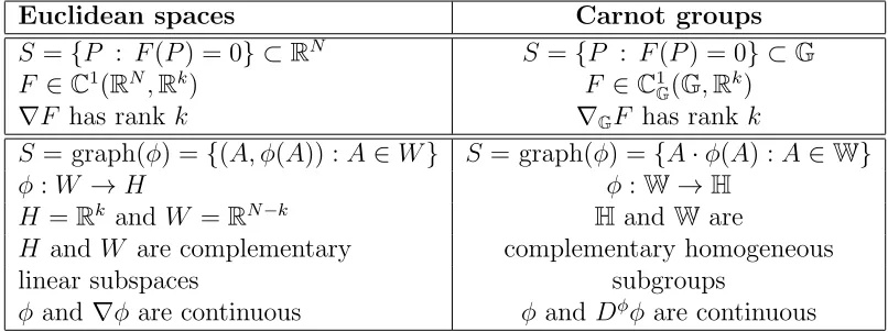
Differently from the Euclidean case where settingC1surfaces can be locally viewed as non-critical level sets ofC1-functions or,equivalently, graphs of
C1 maps between complementary linear subspaces, in Carnot groups the corresponding notion of G-regular surface is not
equivalent to that of intrinsic graph any more. The objective of our research is to study the equivalence of these natural definitions in Carnot groups.
However, thanks to Implicit Function Theorem, proved in [44] for the Heisenberg group and in [45] for a general Carnot group (see also Theorem 1.3, [70]) it follows that
S is a G-regular surface =⇒ S is (locally) the intrinsic graph of a mapφ. Here we say that φ is a parametrization of the G-regular surface.
Consequently, our main purpose is the following fact: given an intrinsic graph of conti-nuous map φ, we want to find necessary and sufficient assumptions on φ in order that the opposite implication is true.
complementary subgroups W and M of G. More precisely, a function is intrinsic differen-tiable if it is well approximated by appropriate linear type functions, denoted intrinsic linear functions.
When W and M are both normal subgroup, the notion of intrinsic differentiability cor-responds to that of P-differentiability.
The title of the thesis is: “Intrinsic differentiability and Intrinsic Regular Surfaces in Carnot groups”. We show that the intrinsic graph of uniform intrinsic differentiable maps is (locally) a G-regular surface. In particular, the original contributions of the author in collaboration with R. Serapioni are illustrated in Chapter 3.
Our aim is to examine the most basic properties of submanifolds inGfrom the viewpoint of Geometric Measure Theory, considering for instance perimeter measures, area formulae, parametrizations, etc.
In the last fifty years many authors have tried to develop a Geometric Measure Theory in Carnot groups or more generally in CC spaces (see [33], [34], [72], [81], [97]). The first result in this sense probably traces back to the proof of the isoperimetric inequality in the Heisenberg group [84] (see also [20], [48]). An essential item of Geometric Measure Theory such as De Giorgi’s notion of perimeter [30], [31] has been extended in a natural way to CC spaces (see [20], [68], [43], [29], [16], [54]). In particular, in Carnot groups the G-perimeter of a measurable set E ⊂Ω is defined as
|∂E|G(Ω) := sup
Z
E
divGφ dLN :φ∈
C1c(Ω, HG),|φ(P)| ≤1
where divGφ:=Pm
j=1Xjφj.
The perimeter measure has good natural properties, such as an integral representation [79] in case of sets with smooth boundary or its (q−1)-homogeneity in Carnot groups setting. More generally, it is also possible to give a good definition of functions of bounded variation [16], [20], [36], [43], which fits the one given for functions in general metric spaces [75]. The theory of minimal surfaces has been investigated [25], [19], [48], [85], and also differentiability of Lipschitz maps [83], [24], [106]; fractal geometry [10]; area and coarea formulae [43], [69], [78] and the isoperimetric problem [64], [90], [53] provided prosperous research themes. However, basic techniques of classical Euclidean Geometry do not admit any counterpart in the CC settings, like Besicovitch covering theorem [89], while many others are still open or only partially solved.
In Section 1.1 we recall the definition of Carnot-Carath´eodory distance and the Chow-Rashevsky theorem, and then in Section 1.2 we go to a brief analysis of the Lie groups and their Lie algebras of the left-invariant vector fields. Here we present some fundamental results proved in [107]. In particular, Theorem 1.2.4 states the exponential map is a global diffeomorphism from the Lie algebra g of a Lie group G toG.
Therefore in Carnot groups any point P ∈ G can be written in a unique way as P = exp(p1X1+· · ·+pNXN) and we identify P with (p1, . . . , pN) and Gwith (RN,·), where the
group operation· is determined by the Baker-Campbell-Hausdorff formula. In particular, in Section 1.3.3, using well-behaved group of dilations, we equip Carnot groups with an explicit group law (see Theorem 1.3.7).
A very special emphasis is given to the examples. In Section 1.4 we introduce and discuss a wide range of explicit Carnot groups of step 2. Some of them have been known in specialized literature for several years, such as the Heisenberg groups [21], [98]; the free step 2 groups [17]; the H-type groups [58]; the H-groups in the Sense of M´etivier [74]; the complexified Heisenberg group [87]. Following [17], we show that these Carnot groups are naturally given with the data on Rm+n of n suitable linearly independent and skew-symmetric matrices of
order m.
In Chapter 2 we provide the definitions and some properties about the differential calculus within Carnot groups.
After a brief description of complementary subgroups of a Carnot group (Section 2.1), we analyze the notion of H-linear maps. In particular, in Section 2.2.2 we investigate the alge-braic conditions under which either surjective or injectiveH-linear functions are respectively H-epimorphisms or H-monomorphisms. Here we present some results obtained in [70].
In Section 2.3 we give a detailed description of Pansu differentiability, with particular emphasis on C1
G functions. Lemma 2.3.7 contains an estimate on horizontal difference
quo-tients of C1G functions which will be crucial in the proof of Theorem 3.1.1, while the main result of this section is Whitney Extension Theorem 2.3.8: its proof was proved in [44] for Carnot groups of step 2 only, but here we give a complete one which is similar.
Then we define and characterize the notion of BVG function and of locally finite G -perimeter set. In particular, Theorem 2.3.14 states the -perimeter measure equals a constant times the spherical (q−1)-dimensional Hausdorff measure restricted to the so-called reduced boundary (Definition 2.3.6) when G is step 2 Carnot group.
In Section 2.4 we introduce one of the main objects of the book, namely G-regular surfaces. This part is taken from a recent paper of Magnani [70]. In particular, Theorem 2.4.3 and 2.4.4 describe all regular surfaces of the Heisenberg groups and of complexified Heisenberg group, respectively.
in this sense is Theorem 2.4.7, whence it follows that the reduced boundary of a locally finite G-perimeter set, up to Hq−1-negligible sets, is contained in a countable union of G-regular hypersurfaces.
In Section 2.5 we talk about intrinsic graphs theory. Implicit Function Theorem 2.5.4 shows that any regular surface locally admits a parametrization. Following the recent papers [39], [38], [94] we discuss about the intrinsic Lipschitz graphs and some their properties. We also mention the paper [42], where this concept appears for the first time when G is an Heisenberg group.
In Section 2.6, we give the general definition of intrinsic differentiability and then we provide the basic tools for the analysis of parametrizations of G-regular surfaces. Namely, for any fixed continuous function φ :E ⊂W → M where M is horizontal subgroup (i.e. its Lie algebra is contained in horizontal layer of G), it is possible to introduce a stronger, i.e. uniform, notion of intrinsic differentiability in a Carnot group G=W·M.
The main item of Chapter 3 is Theorem 3.1.1, where we prove that given a continuous map φ:E ⊂W→MwhereM is horizontal subgroup, it parametrizes aG-regular surface if and only if φ is a uniform intrinsic differentiable map. Moreover Theorem 3.1.5 states that the class of uniform intrinsic differentiable functions is a large class of functions. Indeed it includes the class of C1 functions.
We want to stress in particular the importance of the operatorDφ, which appears in the
proof of Theorem 3.1.1 and which seems to be the correct intrinsic replacement of Euclidean gradient for C1 surfaces.
In Heisenberg groups, it is known after the results in [7], [15] that the intrinsic differen-tiability of φis equivalent to the existence and continuity of suitable ‘derivatives’ Djφφ of φ. The non linear first order differential operators Djφ were introduced by Serra Cassano et al. in the context of Heisenberg groups Hn (see [95] and the references therein). Following the notations in [95], the operators Dφj are denoted as intrinsic derivatives of φ and Dφφ, the
vector of the intrinsic derivatives of φ, is the intrinsic gradient of φ.
Regarding the operator Dφ, we also mention the papers [13], [14], [23], [80], [96] whenG is an Heisenberg group.
In Section 3.2 we analyze the G-regular hypersurfaces in a particular subclass of 2 step Carnot groups. More precisely, we characterize the uniform intrinsic differentiable map φ :E ⊂ W→ M where M is 1 dimensional subgroup of G (and consequently horizontal) in terms of suitable notions of weak solution for the non-linear first order PDEs’ system
(2) Dφφ =w inE,
provided φ and w are locally Lipschitz continuous. In our case φ and w are supposed to be only continuous then the classical theory breaks down. On the other hand broad* solution of the system (2) can be constructed with a continuous datum w.
More specifically, in Theorem 3.2.7 we prove that the intrinsic graph of continuous map φ is a regular surface if and only if φ is broad* solution of (2) and it is 1/2-little H¨older continuous. We also show that these assumptions are equivalent to the fact that φ and its intrinsic gradient Dφφ can be uniformly approximated by
C1 functions.
Acknowledgments. Ringrazio vivamente il mio advisor, il Prof. Raul Serapioni, sia per la sua disponibilit´a, sia per il supporto che ho ricevuto da lui in questi anni di dottorato sopratutto a livello umano.
Ringrazio i referee: il Prof. B.Franchi e il Prof. D.Vittone per il tempo dedicato al mio lavoro. I miei ringraziamenti vanno all’Universit´a di Trento per il supporto durante i miei anni di dottorato e in particolare al Prof. F.Serra Cassano.
Vorrei estendere la mia gratitudine a chi mi ha introdotto in questo percorso: il Prof. D. Mugnai dell’Universit´a di Perugia con cui mi sono laureata e ho pubblicato il mio primo articolo. Un ringraziamento particolare alla Prof.ssa R. Vincenti per i suoi ottimi consigli e disponibilit´a e al Prof. K. Diederich che ho conosciuto durante il corso estivo a Perugia nel 2013.
Carnot groups
In this chapter, we introduce the main notations and the basic definitions concerning with vector fields: algebras of vector fields, exponentials of smooth vector fields, Lie brackets. Then we study Lie groups and the Lie algebra of their left invariant vector fields. Finally, we introduce the main geometric structure investigated throughout the thesis: the Carnot groups. We will take most of the material from [17], [69], [95], [105].
In Section 1.1 we provide a brief exposition of general features concerning Carnot Carath´ eo-dory spaces (see [49], [78]); we recall the definitions of subunitary curve and of Carnot Carath´eodory metric, or cc-metric in short, which is an actual distance thanks to Theorem 1.1.6, so-called Chow-Rashevsky Theorem. Here Rashevsky in [86] and Chow in [26] inde-pendently proved that a sufficient condition for connectivity is the distribution of subspaces Lie generating the whole tangent space at every point.
Section 1.2 is entirely concerned with Lie groups and Lie algebras: we recall some ba-sic facts about Lie groups, providing all the terminology and the main results about the left invariant vector fields, the homomorphisms, the exponential map, the Baker-Campbell-Hausdorff formula (see the monographs [27] and [102] for more references).
The importance of Lie algebras lies in the fact that there is a special finite dimensional Lie algebra intimately associated with each Lie group, and that properties of the Lie group are reflected in properties of its Lie algebra. For instance, the connected, simply connected Lie groups are completely determined (up to isomorphism) by their Lie algebras. Therefore the study of these Lie groups is limited in large part to a study of their Lie algebras. Theorem 1.2.1 and Theorem 1.2.4 are examples of this link.
In Section 1.3 we analyze the Carnot groups G with particular emphasis on their most relevant peculiarities, such as dilations and invariant metrics in G. We recall that a Carnot group of step κ is connected, simply connected Lie group whose Lie algebra admits a stepκ stratification. The Heisenberg groupsHk are the simplest but, at the same time, non-trivial
When κ = 1, G is isomorphic to (RN,+) and this is the only commutative Carnot
group. Thus, when we talk about Carnot groups we always consider κ ≥ 2; in this case, through the exponential map, a Carnot group G can be identified with RN, endowed with
a non commutative group operation given by the Baker-Campbell-Hausdorff formula. In particular, in Section 1.3.3 using well-behaved group of dilations we equip Carnot groups with an explicit group law.
In Section 1.3.5 and 1.3.6, we study the left invariant metrics in G, which are equivalent to Carnot-Carath´eodory metric (see Proposition 1.3.6). Non commutative Carnot groups, endowed with their left invariant metric are not Riemannian manifolds, not even locally. In fact they are particular instances of so-called sub Riemannian manifolds (see [11]).
In Section 1.4 we focus our attention on a subclass of Carnot groups of step 2 shown in [17], Chapter 3: we call them groups of class B. To begin with, we show that they are naturally given with the data on Rm+n of n linearly independent and skew-symmetric
matrices of order m. In particular, we show that the set of examples of groups of class B
contains the free step-two groups, H-type groups (see [58]), H-groups in the sense of M´etivier (see [74]).
1.1
Carnot Carath´
eodory spaces
1.1.1
Vector fields on
R
NLetP = (p1, . . . , pN)∈RN and let X1, . . . , Xm be a family of smooth vectors fields on RN
Xj(P) = N
X
i=1
aij(P)∂pi for j = 1, . . . , m
with aij : RN → R smooth functions. We also suppose that X1, . . . , Xm are linearly
inde-pendent. We define HPRN the horizontal subspaces at the point P the subspaces of TPRN
generated by X1(P), . . . , Xm(P). The collection of all horizontal fibers HPRN forms the horizontal subbundleHRN of T
RN.
Given two smooth vector fields onRN X
1, X2 we define thecommutator (or Lie bracket) [X1, X2] as the smooth vector field given byX1X2−X2X1(as common in literature, we tacitly identify vector fields and first order operators); if X1(P) =
PN
i=1ai(P)∂pi and X2(P) =
PN
i=1bi(P)∂pi then in coordinates [X1, X2] is given by [X1, X2](P) =
N
X
i,j=1
aj(P)∂pjbi(P)−bj(P)∂pjai(P)
∂pi.
For example, for the following two vector fields on R3 (whose points are denoted by P = (p1, p2, p3))X1(P) = ∂p1 + 2p2∂p3 and X2(P) =∂p2 −2p1∂p3, we have
[X1, X2](P) = (X1(−2p1)−X2(2p2))∂p3 =−4∂p3.
We say that the vector fields on RN X
1, . . . , Xm satisfy the Chow-H¨ormander condition
if there is an integerκ≥1 such that the set of linear combinations of family of commutators of X1, . . . , Xm up to the length κ, i.e.
X1, . . . , Xm, [Xi1, Xi2],[Xi1,[Xi2, Xi3]], . . . ,[Xi1,[Xi2,[. . . , Xiκ]. . .], 1≤iδ ≤m
is the tangent space to RN at every point of RN.
Remark 1.1.1. LetX1, . . . , Xm be left invariant vector fields onRN. In this case the
Chow-H¨ormander condition is equivalent to
(1.1) dim(span{X1, . . . , Xm,[Xi1, Xi2], . . . ,[Xi1,[Xi2,[. . . , Xiκ]. . .]}(P)) =N
for all P ∈RN.
1.1.2
Carnot Carath´
eodory distance
An absolutely continuous curveγ : [0, T]→RN is asubunit curvewith respect toX
1, . . . , Xm
if it is an horizontal curve, that is if there are real measurable functions h1(t), . . . , hm(t),
t∈[0, T] such that
˙ γ(t) =
m
X
i=1
hi(t)Xi(γ(t)), for a.e. t ∈[0, T],
and if Pm
i=1h 2
i ≤1.
Definition 1.1.1. We define the Carnot-Carath´eodory distance (cc-distance) between the points P, Q∈RN as
dcc(P, Q) = inf
T ≥0 : there is a subunit curve γ : [0, T]→RN with γ(0) =P, γ(T) = Q .
If the above set is empty we put dcc(P, Q) =∞.
Using the same approach followed in [78], our next task is to prove the following result:
Proposition 1.1.2. Let Ω⊂RN be an open set. If d
cc is finite, i.e. dcc(P, Q)<∞ for all
P, Q∈RN, then (Ω, d
We need two lemmas. If Xj(P) =
PN
i=1aij(P)∂pi for j = 1, . . . , m, then we shall write the coefficients aij in the (N ×m) matrix
B(P) :=
a11(P) . . . a1m(P)
..
. . .. ... aN1(P) . . . aN m(P)
and we define its norm as
kBk:= sup
h∈Rm,|h|≤1
|Bh|.
Notice that Pm
i=1hi(t)Xi(γ(t)) = B(γ(t))h(t) forh(t) = (h1(t), . . . , hm(t)) andt ∈[0, T].
Lemma 1.1.3. Let Ω⊂ RN be an open set. Let P ∈Ω and r >0 be such that U(P, r) :=
{Q∈RN| |Q−P| < r}
bΩ . Moreover let α:= supQ∈U(P,r)kB(Q)k and γ : [0;T]→Ω be a subunit curve such that γ(0) =P. IfαT < r then γ(t)∈U(P, r) for all t∈[0;T].
Proof. By contradiction we suppose that ¯
t:= inf{t∈[0, T] : γ(t)∈/ U(P, r)} ≤T. Then
|γ(¯t)−P|=
Z ¯t
0 ˙ γ(τ)dτ =
Z ¯t
0
B(γ(τ))h(τ)dτ
≤
Z ¯t
0
|B(γ(τ))h(τ)|dτ ≤
Z ¯t
0
kB(γ(τ))k|h(τ)|dτ
≤¯tα≤T α < r.
Consequently γ(¯t) ∈ U(P, r) because U(P, r) is open and this is in contradiction with the definition of ¯t.
Lemma 1.1.4. Let Ω⊂RN be an open set and let K ⊂Ω be a compact set. Then there is
β >0 such that
(1.2) dcc(P, Q)≥β|P −Q| for all P, Q∈K.
Proof. Fix P, Q ∈ K and let γ : [0, T] → Ω be a subunit curve from P to Q. We choose >0 in order that if we put K :={P ∈Ω : minQ∈K|P −Q| ≤}then K bΩ. Moreover
if we define r:= min{,|P −Q|}, then
|γ(T)−γ(0)|=|P −Q| ≥r,
Now we consider two case: r= orr =|P −Q|. If r= then T ≥
α ≥
αρ|P −Q|
where ρ:= supP,Q∈K|P −Q|. If r =|P −Q| then T ≥ |P −Q|/α. As a consequence by the
definition of dcc we get
dcc(P, Q)≥T ≥min
1 α,
αρ
|P −Q|
then the thesis follows with β := minn1
α, αρ
o
. Now we are able to prove Proposition 1.1.2.
Proof. It is clear that dcc(P, P) = 0. Moreover if P 6=Q by (1.2) it follows dcc(P, Q)>0.
The symmetry property dcc(P, Q) = dcc(Q, P) follows from the fact that ifγ : [0, T]→Ω
is a subunit curve then ¯γ(t) =γ(T −t) is a subunit curve too.
Finally, if γ1 : [0, T1]→ Ω and γ2 : [0, T2] →Ω are subunit curves such that γ1(0) = P, γ1(T1) = G,γ2(0) =Gand γ2(T2) =Q then
γ(t) =
γ1(t) if t ∈[0, T1] γ2(t−T1) if t ∈[T1, T1+T2] is a subunit curve from P toQ. Taking the infimum we get that
dcc(P, Q)≤dcc(P, G) +dcc(G, Q),
i.e. the triangle inequality is true.
Remark 1.1.5. Inequality (1.2) shows that the Euclidean metric is continuous with respect to the cc-metric dcc. The converse is in general not true. For example, consider in R2 the
vector fields X1 = ∂p1 and X2 = a(p1)∂p2, where a : R → R is a Lipschitz map defined as
a(p1) = 0 if p1 ≤0 anda(p1)>0 ifp1 >0. Any couple of points inR2 can be connected by piecewise integral curves of X1 and X2, which therefore induce on R2 a finite cc-metric dcc.
But if p1 <0 then
lim
p2→0
dcc((p1, p2),(p1,0)) = 2|p1| 6= 0.
The following theorem, called Chow-Rashevsky Theorem, gives a sufficient condition in order that dcc is finite. For a proof see for instance [11], Theorem 2.4. or [77], Theorem 1.6.2 Theorem 1.1.6. Let the vector fields X1, . . . , Xm in RN satisfy the Chow-H¨ormander
con-dition. Then any two points in RN can be connected by horizontal curve and hence dcc is a
According to the terminology in [49] (see also [77]), we have the following definition:
Definition 1.1.2. The metric space (RN, d
cc) is called Carnot-Carath´eodory space (CC
space).
The CC spaces satisfying Chow-H¨ormander’s condition are also called Sub-Riemannian spaces. Classical examples of Carnot-Carath´eodory spaces are the Carnot groups (see Section 1.3).
1.2
Lie groups and Lie algebras
Before stating the definition of Carnot groups, we want to briefly recall some basic facts on Lie groups and Lie algebras: a more complete description of these structures can be found in [102], [103], [104], [107].
Definition 1.2.1. A Lie group G is a manifold endowed with the structure of differential group, i.e. a group where the map
G×G3(P, Q) 7−→ P−1·Q∈G is of class C∞.
We denote by 0 the identity of the group, while we define, for any P ∈ G, theC∞ map τP :G→G as
Q7→τP(Q) :=P ·Q.
We callτP the left translation by P.
The general notion of Lie algebra is the following
Definition 1.2.2. A Lie algebra g is a vector space together with a bilinear operation [·,·] :g×g→g,
called the Lie bracket such that, for all X1, X2, X3 ∈g, one has 1. anti-commutativity : [X1, X2] =−[X2, X1]
2. Jacobi identity : [X1,[X2, X3]] + [X2,[X3, X1]] + [X3,[X1, X2]] = 0.
A linear subspaces a ⊂ g is a Lie subalgebra of g if a is closed with respect to [·,·], i.e. [X1, X2] ∈ a for every X1, X2 ∈ a. Given two subalgebras a,b of a Lie algebra g we will denote by [a,b] the vector subspace generated by the elements of{[X, Y] : X ∈a, Y ∈b}.
Definition 1.2.3. A vector fieldX ∈Γ(TG) on a Lie group G is left invariant if X(P) = dτP(X(0)), for all P ∈G
where dτP :TG→TG denotes the differential of the left translation by P.
A vector field X is left invariant if and only if
(Xf)(τPQ) =X(f ◦τP)(Q)
for any f ∈C∞(
G) andP, Q∈G. 1
IfX1, X2 are left invariant vector fields, then the Lie bracket [X1, X2] is also left invariant (see Proposition 3.7 in [107]). This implies that by iterated brackets the left invariant vector fields X1, . . . , Xm generate a Lie algebra.
Precisely, we define the Lie algebra of the Lie group G to be the Lie algebra of left invariant vector fields on G.
This Lie algebra is denoted by g and, for every P ∈G, is the vector space
span{X1, . . . , Xm,[Xi1, Xi2],[Xi1,[Xi2, Xi3]], . . . ,[Xi1,[Xi2,[. . . , Xiκ]. . .]}(P).
gis canonically isomorphic to the tangent spacesT0Gat the identity via the isomorphism T0G3v ←→ X ∈g such that X(P) =dτP(v).
Example 1.2.1. We denote the Heisenberg group H1 =R3 with the group law given by (p1, p2, p3)·(q1, q2, q3) = (p1+q1, p2 +q2, p3+q3+
1
2(p1q2−q1p2)).
Note that (p1, p2, p3)−1 = (−p1,−p2,−p3) and the neutral element of the group is the origin. The Heisenberg group H1 is an example of a Lie group, indeed the map
(P, Q)7→Q−1·P = (p1−q1, p2−q2, p3−q3+ 1
2p2(p1−q1)− 1
2p1(p2−q2)) is of class C∞.
1Let Ω⊂
RN be an open set. We recall that ifX =PNj=1aj∂pj andf : Ω→Ris a differentiable function,
then we denote byXf the function on Ω defined by
Xf(P) =
N
X
j=1
The class of left invariant vector fields can be identified with the tangent space T0H1 to H1 at 0. Hence∂p1, ∂p2 and ∂p3 form a basis ofT0H
1. The corresponding left invariant vector fields X1, X2, Y are
X1(P) = dτP∂p1(0)
X2(P) = dτP∂p2(0)
Y(P) = dτP∂p3(0)
for P = (p1, p2, p3). Consequently, using the fact
dτP(0) =
1 0 0
0 1 0
−1 2p2
1 2p1 1
we obtain
X1(P) = (1,0,− 1
2p2) =∂p1 −
1 2p2∂p3
X2(P) = (1,0, 1
2p1) =∂p2 +
1 2p1∂p3
Y(P) = (0,0,1) = ∂p3
The left invariant vector fields X1, X2, Y form a basis of left invariant vector fields for the Lie algebra ofH1. Moreover, since [X
1, X2] =Y and since any commutator involvingX1, X2 more than twice is identically zero, then the Lie algebra of H1 is span{X1, X2,[X1, X2]}.
1.2.1
Homomorphisms and isomorphisms
There is a special finite dimensional Lie algebra intimately associated with each Lie group, and the properties of the Lie group are reflected in properties of its Lie algebra. Here we show their connection in terms of Lie group homomorphism and Lie algebra homomorphism (see [62], [107]).
Definition 1.2.4. Let (G,·) and (H, ?) be Lie groups. A map F : G → H is said a Lie group homomorphism if it belongs to C∞ and it is a group homomorphism, i.e.
F(P ·Q) = F(P)? F(Q), for all P, Q∈G.
A mapF is an isomorphism of Lie groups if it is a Lie groups homomorphism and a diffeomor-phism of differentiable manifolds. An isomordiffeomor-phism ofGonto itself is called an automorphism of G.
Definition 1.2.5. Let (g,[·,·]g) and (h,[·,·]h) be Lie algebras. A map f : g → h is said a
A map f is an isomorphism of Lie algebras if it is a bijective homomorphism of Lie algebras. An isomorphism ofg onto itself is called an automorphism of g.
The first connection between Lie groups and their Lie algebras is that each Lie group homomorphism indices a Lie algebra homomorphism: if F : G → H is a Lie group homo-morphism, we have that F(0) = 0 and the differential at the identity dF0 :T0G→T0His a linear transformation which preserves the bracket operation.
Viceversa, we have the following results:
Theorem 1.2.1 ([107], Theorem 3.27). Let G and H be two Lie groups with Lie algebras
g and h, respectively. Assume G simply connected. Let f : g → h be a Lie algebra ho-momorphism. Then there exists a unique Lie group homomorphism F : G → H such that
dF =f.
Theorem 1.2.2 ([107], Corollary 3.28). If simply connected Lie groups G and H have iso-morphic Lie algebras, then G and H are isomorphic.
1.2.2
Exponential map
In the theory of Lie groups we define the exponential map exp :g→Gas the map from the Lie algebra g of Lie group G toG, given by
exp(X)(P) :=γPX(1) where γX
P :R→Gis the (unique) solution of the following Cauchy problem
(1.3)
˙
γ(t) =X(γ(t)) γ(0) = P
We recall the following basic result proved in [107], Theorem 3.31:
Theorem 1.2.3. Let G be a Lie group with Lie algebrag. IfX ∈g then 1. exp((t+s)X) = exp(tX)·exp(sX) for all t, s∈R
2. exp(−X) = (exp(X))−1
3. exp :g→G is smooth and (dexp)0 is the identity map, (dexp)0 =idg :g→g
so exp gives a diffeomorphism of a neighborhood of 0 in g onto a neighborhood of 0 in
4. the left invariant vector fields are complete. 2
From the unique solvability of the Cauchy problem (1.3) related to smooth vector fields 1. exp(−tX)(P) = exp(t(−X))(P)
2. exp(−tX) exp(tX)(P)=P
3. exp((t+s)X)(P) = exp(tX) exp(sX)(P) 4. exp((ts)X)(P) = exp(t(sX))(P)
for every X ∈TG,P ∈G and t, s ∈R.
Moreover if G and H are two Lie groups with Lie algebras g and h, respectively, and F :G→H is a Lie group homomorphism, then the following diagram is commutative:
g −−−→
dF h
exp
y
y
exp
G −−−→F H
Example 1.2.2 (The exponential map on H1). Let us consider once again the Heisenberg groupH1. In Example 1.2.1, we showed that a basis for its Lie algebrahis given byX1, X2, Y where X1 = ∂p1 −
1
2p2∂p3, X2 =∂p2 +
1
2p1∂p3 and [X1, X2] = Y = ∂p3. Let us construct the
exponential map. We set, for (q1, q2, q3)∈R3
Z :=q1X1 +q2X2+q3Y =
q1 q2
−1
2q1p2+ 1
2q2p1+q3
.
Hence for fixedP = (p1, p2, p3)∈H1, we have
exp(Z)(P) = γPZ(1), where γZ
P(t) = γ(t) = (γ1(t), γ2(t), γ3(t)) is the solution of the Cauchy problem (1.3) , i.e.
˙
γ(t) = (q1, q2, q3− 12q1γ2(t) + 12q2γ1(t)) γ(0) = P
2A smooth vector fieldX on a Lie group
Gis complete if, for everyP ∈G, the integral curveγ ofX
Solving the above system of ODE’s, one gets
exp
q1 q2
−1
2q1p2+ 1
2q2p1+q3
(P) =
p1+q1 p2+q2
p3+q3+ 12(p1q2−p2q1)
.
Example 1.2.3 (Pyramid-shaped vector fields). Let us consider the Lie algebraTRN of the
vector fields on RN equipped with the product [X1, X2] =X1X2−X2X1. We consider in RN vector fields of the following type
(1.4) X =
N
X
j=1
aj(p1, . . . , pj−1)∂pj,
where a1 = constant.
The functionaj only depends on the variablesp1, . . . , pj−1whenj >1. Roughly speaking, such a vector field is pyramid-shaped,
X =
a1 a2(p1) a3(p1, p2)
.. .
aN(p1, . . . , pN−1)
For instance, the vector fields X1, X2, Y in above example have this form.
For any smooth vector field X of the form (1.4), the map (P, t) 7→ exp(tX)(P) is well defined for every P = (p1, . . . , pN) ∈RN and t ∈R and can be easily computed. Indeed, if γX
P =γ = (γ1, . . . , γN) is the solution to the Cauchy problem
˙
γ(t) = X(γ(t)) γ(0) =P
then ˙γ1(t) = a1 and ˙γj(t) =aj(p1, . . . , pj−1) forj = 2, . . . , N. As a consequence,
γ1(t) =p1+ta1, γj(t) =pj +
Z t
0
aj(γ1(s), . . . , γj−1(s))ds
and γj(t) is defined for every P ∈ RN and t ∈R. Moreover γj(t) only depends on the first
components p1, . . . , pj of P = (p1, . . . , pN) for j = 1, . . . , N. Let us put A1(t) :=ta1 and for j = 2, . . . , N
Aj(p1, . . . , pj−1, t) :=
Z t
0
Then, for all P = (p1, . . . , pN)∈RN we conclude that
exp(X)(P) =
p1 +A1(1) p2+A2(p1,1)
.. .
pN +AN(p1, . . . , pN−1,1)
and the mapP 7→exp(X)(P) is a global diffeomorphism of RN onto
RN.
1.2.3
The Baker-Campbell-Hausdorff formula
The algebraic structure ofg determines that of G, and precisely
exp(X1) exp(X2) = exp(C(X1, X2)), for all X1, X2 ∈g
whereC(X1, X2) is given by the following formula, called Baker-Campbell-Hausdorff formula (1.5)
C(X1, X2) = X1+X2+ 1
2[X1, X2] + 1
12[X1,[X1, X2]]− 1
12[X2,[X1, X2]]
− 1
48[X2,[X1,[X1, X2]]]− 1
48[X1,[X2,[X1, X2]]] +{brackets of height≥5}.
C(X1, X2) is an infinite linear combination of X1, X2 and their iterated commutators. It defines a binary operation ing whenever the series converges.
Example 1.2.4. Let g be an abelian Lie algebra, i.e. a Lie algebra such that [X1, X2] = 0 for all X1, X2 ∈g. Then
C(X1, X2) =X1+X2
and consequently exp(X1) exp(X2) = exp(X1+X2) for all X1, X2 ∈g.
Example 1.2.5 (The Baker-Campbell-Hausdorff formula on H1). Let ξ, η ∈ R3 and Z := X1+X2+Y whereX1, X2, Y is the basis for the Lie algebra of Heisenberg groupH1 defined in Example 1.2.1. We explicitly write down C(ξZ, ηZ) in H1, thus obtaining
C(ξZ, ηZ) =ξZ+ηZ+ 1
2[ξZ, ηZ] + 1
12[ξZ,[ξZ, ηZ]] +. . . =ξZ+ηZ+ 1
2[ξZ, ηZ]
(since any commutator involving X1, X2 more than twice is identically 0) =ξ1X1+ξ2X2+ξ3Y +η1X1+η2X2+η3Y
+ 1
2[ξ1X1+ξ2X2 +ξ3Y , η1X1+η2X2+η3Y] (here we use [X1, X2] =Y, [X1, Y] = [X2, Y] = 0) = (ξ1+η1)X1+ (ξ2+η2)X2+ (ξ3+η3+
1 2ξ1η2−
which is the group operation in H1.
1.2.4
Nilpotent groups
Definition 1.2.6 ([27]). Let g be a Lie algebra. For each s∈N we define by induction the following sequence of subspaces
g(s) :=g g(s+1) := [g(s),g].
If there exists a positive integer κ∈Nsuch thatgκ 6={0} and g(κ+1) ={0} we say thatg is
a nilpotent Lie algebra. The integer κ is called the step of g. A Lie groupG is nilpotent if its Lie algebra is nilpotent..
Notice that if gis nilpotent of κ step, then for all s ∈ {1, . . . , κ}the subalgebra g(s+1) is strictly contained in g(s).
Theorem 1.2.4 ([27], Theorem 1.2.1). LetGbe a connected, simply connected nilpotent Lie group, with Lie algebra g. Then
1. The exponential map exp :g→G is an analytic diffeomorphism.
2. The Baker-Campbell-Hausdorff formula holds for all couple of elements of g.
Definition 1.2.7. Let G be a connected, simply connected nilpotent Lie group, with Lie algebrag. Let{X1, . . . , XN}be a basis forg. A system ofexponential coordinates associated
with the basis{X1, . . . , XN} of g is the map Ψ :RN →G
Ψ(p1, . . . , pN) := exp N
X
i=1 piXi
!
.
An important application of Theorem 1.2.4 involves coordinates on G. Since the expo-nential map exp : g → G is a global diffeomorphism, the map Ψ is also a diffeomorphism. Consequently, any P ∈G can be written in a unique way as P = exp(p1X1 +· · ·+pNXN)
and we can identify P with the N-tuple (p1, . . . , pN)∈RN.
Using C(·,·) the Baker-Campbell-Hausdorff formula (1.5), we define a group law on RN
as follows: let (p1, . . . , pN),(p01, . . . , p
0
N)∈RN. If
C
N
X
i=1 piXi,
N
X
i=1 p0iXi
!
=
N
X
i=1 qiXi
then
(p1, . . . , pN)·(p01, . . . , p
0
N) := (q1, . . . , qN).
Example 1.2.6. The Heisenberg group H1 (see Example 1.2.1) is an example of 2 step nilpotent Lie group.
Example 1.2.7(A non-polynomial non-nilpotent Lie group onR2). The following operation onR2
(p1, p2)·(q1, q2) = (p1+q1, q2+p2eq1)
defines a Lie group structure where (p1, p2)−1 = (−p1,−p2e−p1). Moreover a basis of the Lie algebra associated is
Y1 =∂p1 +p2∂p2, Y2 =∂p2
Hence, the Lie algebra is not nilpotent, for [Y2, Y1] =Y2, so that, inductively, [. . .[Y2, Y1], Y1], Y1]. . . Y1]
| {z }
k times
=Y2 for all k∈N.
1.3
Carnot groups of step
κ
We now enter into the core of the chapter by introducing the central definition of this thesis, i.e. Carnot groups. For a general account see e.g. [17], [35], [62], [95], [104], [103].
Definition 1.3.1. A Carnot group G = (G,·, δλ) of step κ is a connected and simply
con-nected Lie group whose Lie algebragadmits a stratification, i.e. a direct sum decomposition
g=g1⊕g2 ⊕· · ·⊕gκ. The stratification has the further property that the entire Lie algebra
g is generated by its first layer g1, the so-called horizontal layer, that is
(1.6)
[g1,gi−1] =gi if 2≤i≤κ
[g1,gκ] ={0}
where [g1,gi] is the subspaces of g generated by the commutators [X, Y] with X ∈ g1 and Y ∈gi.
By Theorem 1.2.4, we can identify G with (RN,·, δ
λ), where the group operation · is
determined by the Baker-Campbell-Hausdorff formula (see Section 1.2.3) and the family of automorphisms {δλ}λ of G is defined in Section 1.3.2.
Let X1, . . . , Xm1 be a base for g1. The subbundle of the tangent bundle TG that is
spanned by the vector fields X1, . . . , Xm1 plays a particularly important role in the theory,
it is called the horizontal bundle HG; the fibers of HGare
HGP = span{X1(P), . . . , Xm1(P)}, P ∈G.
Ifv =Pm1
i=1(v1)iXi(P) andw=
Pm1
i=1(w1)iXi(P) are inHG, then hv, wiP :=
Pm1
i=1(v1)i(w1)i and |v|2
P := hv, viP. We will write, with abuse of notation, h·,·i meaning h·,·iP and | · |
meaning | · |P.
The sections ofHGare calledhorizontal sections, a vector ofHGP is anhorizontal vector
while any vector in TGP that is not horizontal is a vertical vector. Each horizontal section
φ defined on an open set Ω⊂G can be written as φ=Pm1
i=1φiXi, where its coordinates are functions φi : Ω→R. When considering two such sections φ and ψ, we will write hψ, φi for
hψ(P), φ(P)iP.
Remark 1.3.1. Let G be a Carnot group of step κ and let {X1, . . . , Xm1} be a basis of the
horizontal layer g1. By (1.6) we know that X1, . . . , Xm1 generates g by commutations and
consequently X1, . . . , Xm1 satisfy Chow-H¨ormander condition (1.1).
1.3.1
Uniqueness of stratifications
The stratification of a Lie algebra is unique up to isomorphism. Hence, also the structure of a Carnot group is essentially unique:
Proposition 1.3.2 ([63], Proposition 1.17). Let G be a Carnot group with Lie algebra g. Suppose that g has two stratification, g=h1 ⊕ . . . ⊕ hκ and g=h01 ⊕ . . . ⊕ h
0
r.
Then κ=r and there is a Lie algebra automorphism f :g→g such that
f(hs) =h0s, for all s= 1, . . . , κ.
Proof. We begin observing the following simple fact (see Lemma 1.16 in [63]): if g =h1 ⊕ . . . ⊕ hκ, then g is nilpotent of stepκ (see Definition 1.2.6) and g(s) =hs ⊕ . . . ⊕ hκ.
Consequently, g(s) =h
s ⊕ . . . ⊕ hκ =h0s ⊕ . . . ⊕ h0r and soκ=r.
Now we consider the quotient mappings πs :g(s) →g(s)/g(s+1). We have that its
restric-tions πs|hs :hs→g
(s)/g(s+1) and π
s|h0
s :h
0
s→g(s)/g(s+1) are linear isomorphisms.
For X ∈hs and s= 1, . . . , κ, definefs:hs→h0s as
fs(X) := πs|h0
s
−1
◦ πs|hs
(X). More precisely, forX ∈hs and Y ∈h0s
(1.7) fs(X) =Y ⇐⇒ X−Y ∈g(s+1)
In this way we can define a linear map f : g→ g. This is clearly a linear isomorphism and f(hs) = h0s for each s= 1, . . . , κ.
Consequently, it remains to show that f preserves brackets, i.e. f([X, Y]) = [f X, f Y], for all X, Y ∈ g. Let X, Y ∈ g with X =Pκ
s=1Xs and Y =
Pκ
s=1Ys such that Xs, Ys ∈hs. Then
f([X, Y]) =
κ
X
s,l=1
f([Xs, Yl]), [f X, f Y] = κ
X
s,l=1
Therefore it sufficient to prove that
(1.8) f([Xs, Yl]) = [f Xs, f Yl] forXs∈hs, Yl ∈h0l
First, notice that
[Xs, Yl]−[f Xs, f Yl] = [Xs−f Xs, Yl]−[f Xs, f Yl−Yl]∈g(s+l+1)
because, on the other hand, Xs −f Xs ∈ g(s+1), Yl ∈ h0l and consequently [Xs−f Xs, Yl] ∈
g(s+l+1); on the other hand, f X
s∈h0s, f Yl−Yl ∈g(l+1) and so [f Xs, f Yl−Yl]∈g(s+l+1).
Then by (1.7) and since [Xs, Yl]∈hs+l and [f Xs, f Yl]∈h0s+l
f([Xs, Yl]) = [f Xs, f Yl] ⇐⇒ [Xs, Yl]−[f Xs, f Yl]∈g(s+l+1)
i.e. (1.8) holds and so f preserves brackets.
Example 1.3.1. Not all nilpotent Lie algebras admit a stratification, see [51]. Indeed, consider the 7-dimensional Lie algebra g generated by X1, . . . , X7 with only non trivial brackets
[X1, X2] =X3, [X1, X3] = 2X4, [X1, X4] = 3X5, [X2, X3] =X5, [X1, X5] = 4X6, [X2, X4] = 2X6, [X1, X6] = 5X7, [X2, X5] = 3X7, [X3, X4] =X7. This Lie algebra g is not stratifiable.
1.3.2
The dilation structure
The construction of the dilation structure deeply uses the stratification of the algebra g =
g1 ⊕ · · · ⊕ gκ. We denote by δλ :g→gthe family of (non isotropic) dilation defined by
δλ
κ X
i=1 Xi
:=
κ
X
i=1
λiXi, λ≥0
where X =Pκ
i=1Xi with vi ∈ gi, 1 ≤ i≤ κ. The dilations δλ are automorphisms of g and are uniquely determined by the homogeneity conditions
δλXi :=λiXi, ∀Xi ∈gi, 1≤i≤κ.
Moreover, from the grading, it is obvious that 1. δλη =δλ◦δη;
3. δλ(C(X, Y)) = C(δλX, δλY), where C(·,·) is given by (1.5).
By Theorem 1.2.4, in Carnot groups, the map exp : g → G is a diffeomorphism, so any element P ∈ G can be represented as exp(X) for some unique X ∈ g, and therefore it can be uniquely written in the form
exp
κ
X
i=1 Xi
!
, Xi ∈gi, 1≤i≤κ.
Therefore we can define a one-parameter group of automorphism of G, which we still denote with {δλ}λ≥0 via the formula
δλ exp κ
X
i=1 Xi
!!
:= exp
κ
X
i=1 λiXi
!
,
i.e. exp◦δλ =δλ◦exp.
Let f :G→G, then
X(f ◦δλ)(P) = (δλX)f(δλP), for all P ∈G, λ≥0.
Indeed,
X(f◦δλ)(P) =
d
dtf ◦δλ(P exp(tX))|t=0 = d
dtf(δλP δλexp(tX))|t=0 = d
dtf(δλPexp(tδλX))|t=0 = (δλX)f(δλP).
Then the map δλ :G→G is the unique group homomorphism withδλ as differential, whose
existence is given by Theorem 1.2.1 since G is simply connected.
From the properties of dilations in Lie algebras we immediately deduce the associated ones for dilations of Carnot group:
1. δλη =δλ◦δη, indeed
δλη(P) = exp(δληexp−1(P))
= exp(δλδηexp−1(P))
= exp(δλexp−1(expδηexp−1(P)))
= exp(δλexp−1(δη(P)))
2. δλ(P ·Q) = δλ(P)·δλ(Q) for all P, Q∈G. Indeed
δλ(P Q) = exp δλexp−1(P Q)
= expδλ(C(exp−1P,exp−1Q))
= exp(C(δλexp−1P, δλexp−1Q))
= exp(δλexp−1P) exp(δλexp−1Q))
=δλ(P)δλ(Q).
where C(·,·) is given by (1.5).
1.3.3
The Composition Law of
G
Following [17], in this section we give a structure theorem for the group operation in a Carnot group G (see Theorem 1.3.7).
Let us introduce some notations. Let G be a Carnot group with Lie algebra g such that
g = g1 ⊕ g2 ⊕ · · · ⊕ gκ and, for s = 1, . . . , κ, let ns := dimgs and ms −ms−1 := ns with
m0 = 0 < m1 <· · ·< mκ =N.
We say that a basis X of g is adapted to (g1, . . . ,gκ) if
X = (X11, . . . , Xn11, . . . , X1κ, . . . , Xnκκ )
where ns := dimgs and (X1s, . . . , Xnss ) is a basis for gs for all s= 1, . . . , κ.
Definition 1.3.2. Let G be a Carnot group with Lie algebra g. A system of exponential coordinates Ψ :RN →
Gis a system ofgraded coordinates if it is associated with an adapted basis of g.
Let Ψ : RN →
G be a system of graded coordinates. For simplicity we denote with δλ :RN →RN the dilations read in coordinates, so thatδλ◦Ψ = Ψ◦δλ. Then
(1.9) δλ(P) = (λα1p1, . . . , λαNpN), ∀P = (p1, . . . , pN)∈RN where 1 =α1 =· · ·=αm1 < αm1+1 = 2 ≤ · · · ≤αN =κ.
Now we show some basic properties of homogeneous functions and homogeneous differ-ential operators with respect to the family {δλ}λ which is crucial for the proof of Theorem
1.3.7.
Definition 1.3.3. Let f : RN → R. We say that f is δλ-homogeneous of degree l ∈ R if f
Moreover a non-identically-vanishing linear differential operatorX is calledδλ-homogeneous
of degree l∈R if, for every g ∈C∞(
RN) and λ >0, it holds X(g◦δλ) = λl(Xg)◦δλ.
Remark 1.3.3. Let f be a smooth δλ-homogeneous function of degree l ∈ R and X be a
linear differential operator δλ-homogeneous of degree h∈R. ThenXf is a δλ-homogeneous
function of degreel−h (unless Xf ≡0). Indeed for every P ∈G and λ >0 we have λh(Xf)(δλ(P)) =X(f(δλ(P))) =X(λlf(P)) =λl(Xf)(P).
Definition 1.3.4. Let G = (RN,·, δ
λ) be a Carnot group of step κ where δλ is defined as
(1.9). Then given a multi-index β = (β1, . . . , βN)∈(N∪ {0})N, we define the δλ-length (or
the G-length of β) as
|β|α := N
X
i=1 βiαi,
where α is given by (1.9). Moreover, if P :G→R is a polynomial function (the sum below is intended to be finite), i.e.
P(P) =X
σ
cσPσ, cσ ∈R,3
then we say that
degG(P) := max{|β|α : cβ 6= 0}
is the G-degree or δλ-homogeneous degree of P.
Notice that since P 7→ pj is δλ-homogeneous of degree αj, the function P 7→ Pβ is
δλ-homogeneous of degree |β|α.
Moreover, since ∂pj for j ∈ {1, . . . , N} is δλ-homogeneous of degree αj, the differential
operator Dβ is δλ-homogeneous of degree |β|α.
Proposition 1.3.4 (Smoothδλ-homogeneous functions). Letδλ be as in (1.9). Suppose that
f ∈ C∞(
RN). Then f is δλ-homogeneous of degree l ∈ R if and only if f is a polynomial
function of the form
(1.10) f(P) = X
|β|α=l
fβPβ
with some fβ ∈ R − {0}. As a consequence, the set of the degrees of the smooth δλ
-homogeneous functions is precisely the set of the nonnegative integer numbers
A ={|β|α : β ∈(N∪ {0})N},
with |β|α = 0 if and only if f is constant.
3 Pσ simply meanspα1
1 p α2
2 . . . p αN
Proof. It is clear that every polynomial function of the form (1.10) is δλ-homogeneous of
degreel. Consequently it remains to prove that iff isδλ-homogeneous of degreel ∈R, then
f is a polynomial function of the form (1.10).
If f(Q)6= 0 for some Q∈RN, then l≥0. Indeed, from f(δ
λQ) = λlf(Q) we get
lim
λ→0λ
l
= lim
λ→0
f(δλQ)
f(Q) = f(0)
f(Q) <∞.
Moreover, the continuous andδλ-homogeneous of degree 0 functions are precisely the constant
(non-zero) functions. Indeed,
f(P) =f(δλ(P)) = lim
λ→0+f(δλ(P)) =f(0).
Then we can suppose thatf is a non constant map. ConsequentlyDβf is not identically zero and since Dβf is smooth and δ
λ-homogeneous of degree l− |β|α , we have that l− |β|α≥0.
This result can be restated as follows:
Dβf ≡0 ∀β such that|β|α > l.
Thus f is a polynomial function, i.e. f(P) = P
β∈AfβPβ, where A is a finite set of
multi-indices and fβ ∈R for every β ∈ A. Because f is δλ-homogeneous of degree l, we obtain
X
β∈A
λlfβPβ =λlf(P) = f(δλ(P)) =
X
β∈A
λ|β|αf βPβ.
Hence λlf
β = λ|β|αfβ for every λ > 0, so that |β|α = l if fβ 6= 0. Then f is a polynomial
function of the form (1.10), as desired.
Now we present some elementary properties of the δλ-homogeneous functions.
Lemma 1.3.5. Let δλ be as in (1.9). Let P : RN ×RN → R be a smooth function with
the following property: there is j ∈ {1, . . . , N} such that for all P = (p1, . . . , pN) and
Q= (q1, . . . , qN)
1. P(δλ(P), δλ(Q)) =λαjP(P, Q), for all λ >0
2. P(P,0) = pj
Then
P(P, Q) =
pj+qj if j ∈ {1, . . . , m1} pj+qj+ ˜Pj(P, Q), if j ∈ {m1+ 1, . . . , N}
where P˜j is a polynomial and is the sum of mixed monomials in p1, . . . , pj−1, q1, . . . , qj−1.
Moreover, P˜j(δλ(P), δλ(Q)) = λαjP˜j(P, Q). Finally, P(P, Q) only depends on the pk’s and
qk’s with αk< αj.
Proof. By Proposition 1.3.4, P is a polynomial function of the following type:
P(P, Q) = X
|σ|α+|ρ|α=αj
cσ,ρPσQρ, cσ,ρ ∈R
and by the properties 2. and 3. it follows that pj =P(P,0) =
X
|σ|α=αj
cσ,0Pσ and qj =P(0, Q) =
X
|ρ|α=αj
c0,ρQρ.
Then
(1.11) P(P, Q) = pj +qj +
X
|σ|α+|ρ|α=αj σ,ρ6=0
cσ,ρPσQρ.
We can complete the proof by noticing that the condition |σ|α+|ρ|α =αj, σ, ρ6= 0 is empty
whenj = 1, . . . , m1, whereas it impliesσ = (σ1, . . . , σj−1,0, . . . ,0),ρ= (ρ1, . . . , ρj−1,0, . . . ,0)
when j ≥m1+ 1.
As for the last assertion of the lemma, being σ, ρ6= 0 in the sum in the right-hand side of (1.11), the sum itself may depend only on theσ’s and ρ’s with|σ|α+|ρ|α< αj, hence, on
the pk’s and qk’s with αk< αj.
Lemma 1.3.6. Let δλ be as in (1.9). Let P :RN ×RN →R be a smooth function. Assume
that there is l ≥0 such that for all P, Q∈RN and for all λ >0 such that
P(δλ(P), δλ(Q)) =λlP(P, Q).
Then
P 7→∂qjP(P,0)
is δλ-homogeneous of degree l−αj (unless it vanishes identically).
Proof. By Lemma 1.3.5, P is a polynomial of the following type
P(P, Q) = X
|σ|α+|ρ|α=l
Then, denoting by ej the j-th element of the canonical basis of RN, we obtain
∂qjP(P, Q) =
X
|σ|α+|ρ|α=l
cσ,ρρjPσQρ−ej,
so that, since |ej|α =αj,
∂qjP(P,0) =
X
|σ|α=l−αj ρ=ej
cσ,ρPσ
This ends the proof.
Now, we are in the position to prove the previously mentioned structure theorem for the composition law of a Carnot group.
Theorem 1.3.7. Let G = (RN,·, δ
λ) be a Carnot group of step κ. Then the group
oper-ation · has polynomial component functions. Furthermore, for each P = (p1, . . . , pN), Q =
(q1, . . . , qN)∈RN we have
(P Q)j =
pj +qj, for j = 1, . . . , m1 pj +qj +Qj(P, Q) for j =m1+ 1, . . . , N
and the following facts hold:
1. Qj is a sum of mixed monomials in P, Q.
2. Qj(δλP, δλQ) = λαjQj(P, Q) for all P, Q∈G and λ >0.
3. Qj(P, Q) only depends on thepk’s and qk’s with αk < αj.
More precisely,
(1.12) Qj(P, Q) =
X
l,h
Rjl,h(P, Q)(plqh−phql), for m1 < j ≤N
where Rjl,h are polynomials, homogenous of degree αj−(αl+αh) with respect to group
dila-tions, and the sum is extended to all l, hsuch that αl+αh ≤αj.
Proof. Fixj = 1, . . . , N. We define
Qj :RN ×RN →R Qj(P, Q) = (P Q)j.
Since δλ is an automorphism of G, we get
Moreover, because P ·0 =P, 0·Q=Q, we obtain that
Qj(P,0) =pj, Qj(0, Q) = qj,
Hence we can apply Lemma 1.3.5 to Qj and consequently we obtain that the conditions
1-2-3 hold for all j = 1, . . . , N. Finally (1.12) follows from Proposition 2.2.22 (4) in [17]. It is useful to know that G =G1 ⊕
G2 ⊕ · · · ⊕ Gκ where Gi = exp(gi) = Rni is the ith layer ofG and to write P ∈G as (p1, . . . , pκ) withpi ∈
Gi. According to this
(1.13) P ·Q= (p1+q1, p2+q2+Q2(p1, q1), . . . , pκ+qκ+Qκ((p1, . . . , pκ−1),(q1, . . . , qκ−1)