Optimization Modulo Theories with OptiMathSAT

ICT INTERNATIONALDOCTORALSCHOOL

DEPARTMENT OFINFORMATION ENGINEERING ANDCOMPUTER SCIENCE

U

T

Optimization Modulo Theories

with O

PTI

M

ATH

SAT

PATRICK

TRENTIN

Advisor:

Prof. Roberto Sebastiani

DISI, U

T

, I

In the contexts of Formal Verification (FV) and Automated Reasoning (AR), Satisfiability

Mod-ulo Theories (SMT) is an important discipline that allows for dealing with industrial-level

de-cision problems. Optimization Modulo Theories (OMT) extends Satisfiability Modulo Theories

with the ability to express, and optimize, objective functions.

Recently, there has been a growing interest towards OMT, as witnessed by an increasing

number of applications using, at their core, some OMT solver as main power-horse engine.

However, at present few OMT solvers exist, and the development of OMT technology is still

at an early stage, with large margins of improvement. We identify two major advancement

directions in particular. First, there is a general need for closing the expressiveness gap with

respect to SMT, and provide optimization procedures that can deal with the wider range of

theories supported by SMT solvers. Second, there is an urgent need for more efficient techniques

that can improve on the performance of state-of-the-art OMT solvers, because solving an OMT

problem is inherently more expensive than dealing with its SMT counterpart, often by at least

one order of magnitude.

In this dissertation, we present a variety of techniques that deal with the identified issues and

advance both the expressiveness and the efficiency of OMT. We describe our implementation

of these techniques inside OPTIMATHSAT, a state-of-the-art OMT solver based on

MATH-SAT5, along with its high-level architecture, Input/Output interfaces and configurable options. Thanks to our novel contributions,OPTIMATHSATcan now deal with the single- and the

multi-objective incremental optimization of goals defined over multiple domains –the Boolean, the

mixed Linear Integer and Rational Arithmetic, the Bit-Vector and the Floating-Point domain–

including (Partial Weighted)MAXSMT.

We validate our theoretical contributions experimentally, by comparing the performance of

OPTIMATHSAT against other, competing, OMT solvers. Finally, we investigate the effective-ness of OMT beyond the scope of Formal Verification, and describe an experimental evaluation

comparingOPTIMATHSATwith Finite Domain Constraint Programming tools on

benchmark-sets coming from their respective domains.

Keywords

Acknowledgements

A doctoral thesis is often described as a solitary endeavour; however the long list that follows definitely proves the opposite.

First, I would like to express my sincere gratitude to my advisor Prof. Roberto Sebastiani for the continuous support of my Ph.D. study, for his patience, motivation and brilliant insights. His guidance helped me throughout my entire research and also with writing this thesis. I could not have imagined having a better advisor and mentor for my Ph.D. study. Besides my advisor, I would also like to thank the rest of my thesis committee: Prof. Albert Oliveras, Prof. Luigi Palopoli and Prof. Cesare Tinelli, for taking the time to review this thesis and for their insightful feedback on its contents. After spending so many years at this institution, I feel that I also owe my gratitude to the staff of the ICT Doctoral School and the DISI department of the University of Trento. In particular, I would like to thank the two members of the doctoral school staff, Francesca Belton and Andrea Stenico, and the four members of the technical staff, Alessandro Tomasi, Mario Passamani, Veronica Rizzi and Danilo Severina. All of them have demonstrated, time after time, great dedication to their job as well as a rare inclination for kindness and willingness to help. A special thank goes to Michela Angeli, a former employee of this institution, whose work lifted me from the burden of dealing with the task of organizing my work-related travels and helped me focusing on my research at the early stages of this Ph.D. study.

Second, I would like to thank Dr. Silvia Tomasi who, together with Prof. Roberto Sebas-tiani, laid the foundations for this research and built the first version of OPTIMATHSAT, before advancing her career elsewhere and passing on the torch to me. I would also like to thank the members of the MATHSAT team, namely Dr. Alberto Griggio, Dr. Alessandro Cimatti and Prof. Roberto Sebastiani, as well as the countless people who gave their contribution to MATH-SAT over the years: a significant portion of OPTIMATHMATH-SAT’s success is the consequence of their efforts. I am especially grateful to Dr. Alberto Griggio who has helped me with MATH-SAT5 code and has always shown both an unlimited amount of patience and a gracious sense of humor in all of our interactions, despite the sharp expertise gap among us.

Third, I would like to thank Prof. David Monniaux, who provided me with an opportunity to join his team at VERIMAG as an intern during my Ph.D. study, and provided me with both valuable guidance and feedback regarding this research work and on my research attitude in general.

Dr. Mai Chi Nguyen and Dr. Stefano Teso, whose research provided useful benchmark-sets for OPTIMATHSAT and also helped steering my research efforts towards a fruitful direction. I hold the same amount of gratitude towards those bachelor’s degree students (Luca Gasparetto) and master’s degree students (Filippo Bigarella and Francesco Contaldo) who have seen the potential of this research and decided to cooperate with our research group during their studies. Working with everyone of them as been an invaluable chance of personal growth for me. I am especially grateful towards Francesco Contaldo for his tireless work on theOMT2MZNproject, and also for allowing me to include part of his experimental results in this dissertation.

Fifth, I would like to thank the countless number of people working in my research domain, and those fields closely related to it, for sharing their insightful ideas with the community and helping me to expand my incredibly limited horizons. This thesis builds upon the ideas of many people and I hope that it can contribute to their success by spreading their work even further. I am also grateful towards those researchers and software maintainers who have kindly answered my questions and addressed my bug reports over the past years. Their help often came in when it was needed the most and in exchange for no more than a simple “thank you”.

Last but not the least, I thank my friends for sharing this voyage with me, both those who have always remained at my side over the years as well as those who are now gone forever but have left a piece of themselves in my heart. I would like to deeply thank my parents, Fausto Trentin and Helga Gasser, who have sacrificed pursuing their own life goals in order to support their children even at hardship, and my sisters, Silvia and Deborah Trentin, who have given me the opportunity to gauge at life from different perspectives. I would also like to express my deepest gratitude to my father and mother in law, 蔡崇條 and _吳美_{花, who have welcomed}

me in their family –without any preconception– and have graciously granted me the honor of taking their only daughter, 蔡亞芳, as my beloved wife for the rest of our days. My spouse is my most enthusiastic cheerleader, she is my best friend and she is an amazing wife. Without her cheerful mind, I would be a much grumpier person; without her love and support, I would be lost. I am grateful to my wife not just because she has given up her own life to be at my side, but because she has spent sleepless nights taking care and supporting me in the moments when I most needed it. At long last, her unbending love has given peace to my restless soul, so it only seems right that I dedicate this dissertation to her:

1 Introduction 1

I

Background, State of the Art and Related Work

11

2 Background & State of the Art 13

2.1 Propositional Satisfiability . . . 14

2.2 Satisfiability Modulo Theories . . . 16

2.2.1 The “lazy” SMT Scheme . . . 19

2.2.2 Incremental SMT . . . 23

2.2.3 Theories of Interest . . . 24

2.2.4 Combination of Theories in SMT . . . 28

2.3 Optimization Modulo Theories . . . 29

2.3.1 OMT (LRA ∪ T) . . . 30

2.3.2 OMT (LIA ∪ T) . . . 37

2.3.3 OMT(PB ∪ T)/MAXSMT . . . 38

2.4 Constraint Programming and SAT/SMT/OMT . . . 43

2.4.1 (Finite Domain) Constraint Programming . . . 44

2.4.2 MINIZINC . . . 45

2.4.3 FDCP vs. SAT, SMT and OMT . . . 46

3 Related Work 53

II

Contributions

59

4.2.1 Sorting Networks Approach . . . 65

4.2.2 MAXRESApproach [NB14, BP14] . . . 72

4.3 OMT (BV ∪ T) . . . 77

4.3.1 Signed/unsigned OMT-based Search . . . 82

4.3.2 A signed extension ofOBV-WA[NR16] . . . 84

4.3.3 A signed extension ofOBV-BS[NR16] . . . 85

4.4 OMT (F P ∪ T) . . . 86

4.4.1 OMT-based Search . . . 95

4.4.2 OFP-BS . . . 97

4.5 Incremental OMT . . . 101

4.6 Multi-Objective Optimization . . . 102

4.6.1 MINMAX/MAXMINCombination . . . 103

4.6.2 Multiple-Independent Optimization . . . 103

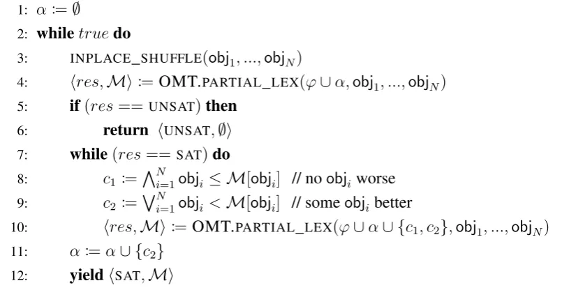
4.6.3 Lexicographic Optimization . . . 107

4.6.4 Pareto Optimization . . . 111

4.7 All-OMT . . . 117

5 OptiMathSAT 121 5.1 Architecture . . . 121

5.2 Compositional Approach . . . 126

5.3 Input/Output Interfaces . . . 127

5.3.1 Extended SMT-LIBV2 Interface . . . 128

5.3.2 MINIZINCInterface . . . 137

5.3.3 API Interface . . . 143

5.4 Configurable Options . . . 152

5.4.1 Input/Output Interface Options . . . 153

5.4.2 OMT-based Search Options . . . 155

5.4.3 Early Termination and Approximate Search Options . . . 157

5.4.4 T-Specific Options . . . 159

5.4.5 Cardinality Constraints Options . . . 163

5.4.6 Multi-Objective Options . . . 165

5.4.7 MINIZINCOptions . . . 167

6 Experimental Evaluations 169 6.1 OMT (LIA ∪ T) Evaluation . . . 170

6.2.1 CGMs with lexicographic OMT . . . 173

6.2.2 CGMs with Un-weighted MAXSMT . . . 176

6.2.3 CGMs with MAXMINOMT . . . 177

6.2.4 LMT with OMT(PB ∪ T) . . . 178

6.3 OMT (BV ∪ T) Evaluation . . . 179

6.4 OMT (F P ∪ T) Evaluation . . . 184

6.5 Incremental and Multi-Objective OMT Evaluation . . . 191

6.6 OMT vs MINIZINC . . . 194

6.6.1 MINIZINCChallenge (2016) . . . 195

6.6.2 OMT Benchmarks . . . 203

7 Applications 209 7.1 OMT Applications . . . 209

7.2 OPTIMATHSAT Applications . . . 213

7.2.1 Learning Modulo Theories . . . 213

7.2.2 Constrained Goal Models . . . 214

7.2.3 WCET . . . 214

7.2.4 Quantum Annealing . . . 216

4.1 SampleF P variable values . . . 89

6.1 Comparison on OMT(LIA)Bounded Model Checking formulas . . . 171

6.2 Comparison on lexicographic OMT formulas of [NSGM16b, NSGM16a] . . . 175

6.3 Comparison on lexic. OMT formulas of [NSGM16b, NSGM16a] with splitting 175 6.4 Comparison on un-weighted MAXSMT formulas from [NSGM16b, NSGM16a] 176 6.5 Comparison on MAXMINformulas from [NSGM16b, NSGM16a] . . . 177

6.6 Comparison on OMT(PB ∪ T)formulas from [TSP17] . . . 178

6.7 Comparison on OMT(BV ∪ T)formulas of [NR16] . . . 181

6.8 Comparison on OMT(F P)formulas . . . 186

6.9 Comparison on multiple-independent OMT formulas of [LAK+14] . . . 192

6.10 Comparison on the MINIZINC Challenge 2016 formulas . . . 196

6.11 MINIZINC Comparison on BMC formulas of [ST15a] . . . 206

2.1 The “lazy” SMT schema . . . 20

2.2 Offline OMT(LRA)procedure of [ST12, ST15a] . . . 32

2.3 Example of the inline OMT(LRA)procedure of [ST12, ST15a] . . . 35

4.1 Simple example of OMT search . . . 67

4.2 Schema of a sorting network relation . . . 68

4.3 Simple example of OMT search with sorting networks . . . 70

4.4 The MAXRESengine in OPTIMATHSAT . . . 73

4.5 F P optimization with Dynamic Attractor . . . 93

4.6 TheOFP-BS algorithm . . . 98

4.7 The functionUPDATE_DYNAMIC_ATTRACTOR() . . . 100

4.8 Example of multiple-independent OMT with OPTIMATHSAT . . . 106

4.9 Lexicographic OMT algorithm based on an unified OMT search . . . 108

4.10 Lexicographic OMT algorithm based on iterated OMT search . . . 110

4.11 The Guided Improvement Algorithm for Pareto OMT [REJ09, BP14] . . . 112

4.12 The Lexicographic Guided Improvement Algorithm for Pareto OMT . . . 116

4.13 ALL-OMT algorithm . . . 118

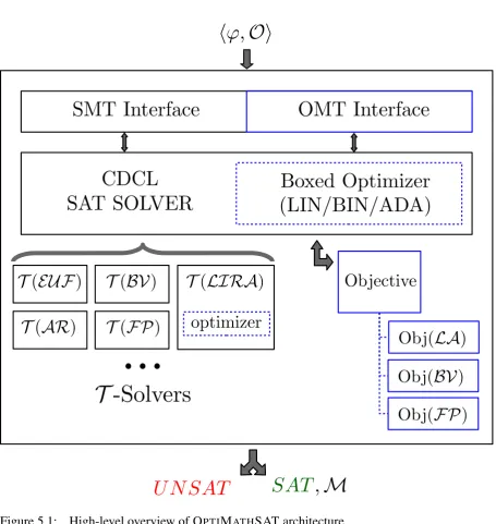
5.1 OPTIMATHSAT Architecture . . . 123

5.2 OMT Interface (Detail) . . . 125

5.3 Extended SMT-LIBV2 example . . . 135

5.4 Extended SMT-LIBV2 example output . . . 136

5.5 MINIZINC Cutstock example . . . 142

5.6 FLATZINCCutstock example . . . 144

5.7 SampleC APIcode. . . 151

6.1 Comparison on OMT(LIA)Bounded Model Checking formulas . . . 172

6.3 Comparison on MAXMINformulas from [NSGM16b, NSGM16a] . . . 177

6.4 Comparison on OMT(PB ∪ T)formulas from [TSP17] (Scatter Plots) . . . . 179

6.5 Comparison on OMT(BV ∪ T)formulas of [NR16] (Scatter Plots) . . . 183

6.6 Comparison on OMT(F P)formulas with linear-search (Scatter Plots) . . . 187

6.7 Comparison on OMT(F P)formulas with binary-search (Scatter Plots) . . . 188

6.8 Comparison on OMT(F P)formulas usingOFP-BS(Scatter Plots) . . . 189

6.9 Comparison on multiple-independent OMT formulas of [LAK+14] (Scatter Plots)193 6.10 Comparison on the MINIZINC Challenge 2016 formulas (Cactus Plot) . . . 197

6.11 Comparison on the MINIZINC Challenge 2016 formulas (Scatter Plots #01) . . 198

6.12 Comparison on the MINIZINC Challenge 2016 formulas (Scatter Plots #02) . . 199

6.13 Comparison on the MINIZINC Challenge 2016 formulas (Scatter Plots #03) . . 200

6.14 Comparison on the MINIZINC Challenge 2016 formulas (Scatter Plots #04) . . 201

6.15 Comparison on the MINIZINC Challenge 2016 formulas (Scatter Plots #05) . . 202

6.16 MINIZINC Comparison on BMC formulas of [ST15a] (Scatter Plots) . . . 205

7.1 Example of Automatic Character Drawing application from [TSP17] . . . 214

Introduction

Satisfiability Modulo Theories (SMT) denotes the problem of deciding the satisfiability of a first-order formula with respect to a combination of decidable first-order theories [BSST09]. The last fifteen years have witnessed the development of very efficient SMT solvers, most of which are based on the so-called lazy-SMT schema that combines the power of modern Conflict-Driven Clause-Learning (CDCL) SAT solvers [MSLM09] with the expressiveness of dedicated decision procedures (T-solvers) for several first-order theories of practical inter-est such as linear arithmetic over the rationals (LRA), the integers (LIA) or their combina-tion (LIRA), non-linear arithmetic over the reals (N LRA) or the integers (N LIA), arrays (AR), bit-vectors (BV), floating-point arithmetic (F P), and their combinations thereof. (See [NOT06, Seb07, BSST09] for an overview.). This has brought previously-intractable problems to the reach of state-of-the-art SMT solvers, so much so that SMT has acquired a prominent role in many applications of industrial interest such as Formal Verification (FV) of hardware and software systems, Automated Reasoning (AR), resource planning, temporal reasoning and scheduling of real-time embedded systems.

A non-exhaustive list of the most recent OMT applications can be found towards the end of this dissertation, while a few examples of less-recent OMT applications can also be found in [NO06, CFG+10, ST12, CGSS13a, LAK+14, BP14, LORR14, ST15a, ST15c, ST17, ST18].

Since the seminal work of Nieuwenhuis and Oliveras in [NO06], which have dealt with the Optimization Modulo Theories problem for first, there has been an increasing interest around this topic. However, the research on OMT still appears to be at an early stage when compared with other, more thoroughly studied, fields such as SMT. In fact, the number of scientific publications in the literature that extend SMT with optimization is fairly limited, [NO06, CFG+_{10, Roc11, ST12, DDMA12, MP13, CGSS13a, LAK}+_{14, LORR14, ST15a], and} there are only a handful of more recent works that can be added to this figure, [BP14, BPF15, ST15b, ST15c, ABCF16, NR16, ST17, AAdB+_{17, ST18, FBB18, KBE18, AAdB}+_{18, TS19],} although we expect more to appear.

To this date, few OMT solvers exist that are also applicable beyond the scope of Partial Weighted MAXSMT, namely BCLT [NO06, BNO+08, Roc11, LORR14], CEGIO [ABCF16,

AAdB+17, AAdB+18], HAZEL[NR16], OPTIMATHSAT [ST12, ST15a, ST15b, ST15c, ST17, ST18, TS19], PULI[KBE18], SYMBA[LAK+14] and Z3 [BP14, BPF15]. To this aim, we ob-serve that most of these solvers focus on different, partially overlapping, niche subsets of Opti-mization Modulo Theories, and employ different standards for their Input/Output interfaces. In practice, the combination of these two factors makes it hard to compare with one another the few OMT solvers in existence.

In what follows we focus on the state of the art prior of the start of this Ph.D. program (November 1st_{, 2014). Then, we make the following observations. Some of these works, such}

as [NO06, CFG+_{10, CGSS13a], are applicable only to Partial Weighted MAXSMT, which is} strictly less expressive than Optimization Modulo Theories with Linear Integer/Rational Arith-metic cost functions [ST15a]. The optimization procedures described by Sebastiani and Tomasi in [ST12, ST15a] and by Li et al. in [LAK+_{14] can only deal with OMT with aLinear Rational}

Arithmetic objective. In contrast, those described by R. O. Vendrel in [Roc11] and Manolios

Verification.

Based on the above considerations on the status of Optimization Modulo Theories before the start of this research, we identify the following improvements as necessary milestones to unleash the full potential of Optimization Modulo Theories and make it further adopted in the context of real-world, industrial-level, applications.

First, there is a general need to bridge the expressiveness gap of Optimization Modulo Theo-ries when compared to Satisfiability Modulo TheoTheo-ries, and go beyond the variousLinear

Arith-meticrestrictions that are currently supported by OMT and MAXSMT solvers. This not only means introducing optimization procedures that can handleMixed Linear Integer and Rational

Arithmeticgoals and combination of theories at the same time, but also objective functions

de-fined in other theories thanLinear Arithmetic, such as the theory of Bit-Vectors and the theory of Floating-Point numbers.

Second, it is necessary to investigate possible approaches for improving the performance of OMT solvers, including methods that are only applicable to objective functions abiding to certain format restrictions (like, e.g., MAXSMT). This goal is easily justifiable by observing that while the leap from SMT to OMT can appear to be quite small from the perspective of an end-user, due to the ease with which a new objective can be both declared and used, in practice solving an OMT problem can be orders of magnitude harder in terms of computational effort than dealing with its SMT counter-part. This is due to the fact that in an SMT solver the search stops as soon as the first feasible solution is hit, whereas in an OMT solver the search is normally terminated only when an optimal solution is found. In practice, dealing with the latter goal is a significantly more daunting task than satisfiability, that can require enumerating multiple suboptimal solutions along the search and also certifying the absence of an improving solution at the end of the optimization search. Therefore, we believe that Optimization Modulo Theories can greatly benefit from the investigation of more efficient techniques that may bring previously intractable applications within the reach of OMT solvers.

A third improvement direction, closely related to the previous goal, isincrementality. This refers to the ability to push and pop both constraints and objectives on the formula stack of an OMT solver, while being able to reuse useful information automatically learned by the OMT solver across multiple optimization searches. This feature, that is widely supported among SMT solvers, can be crucial for achieving significant search speed-up when dealing with applications that require performing a large number of incremental calls to the tool, each bringing small changes to the previous formula.

ability of performing Lexicographic or Pareto-optimization search over a set of constraints. Fifth, we believe it is worth considering whether the range of applications of Optimization Modulo Theories can be extended further beyond its natural Formal Verification (FV) and Au-tomated Reasoning (AR) domains, and to what extent. In this respect, it is worth noting that there are other tool families that allow for optimizing some objective function under a set of constraints, such as Finite Domain Constraint Programming(FDCP) and Mixed Integer Lin-ear Programming (MILP). Among its strengths, Optimization Modulo Theories can rely on

native Boolean reasoning capabilities, that may prove to be an edge when dealing with highly combinatorial problems, and the ability to handle theories that are commonly not supported by tools coming from other research fields, such as the theory of arrays (AR) or the theory of uninterpreted functions with equality (EU F). Previous works, such as [BPV09, BPSV09, BSV10, BPSV12], have already started investigating those applications for which Satisfiability Modulo Theories can be competitive with FDCP and MILP tools. Part of the work described in this thesis is devoted to pushing forward this research work, focusing on Optimization Modulo Theories.

On the whole, the expected benefits from the rise of more efficient and expressive Optimiza-tion Modulo Theories solvers are many-fold.

• In those application fields that already benefit from SMT technology —like, e.g., Formal Verification and AI Planning— the rise of efficient OMT tools should allow for addressing more sophisticate versions of those problems (like, e.g., planning with resource optimiza-tion).

• In those application fields that typically make use of FDCP/MILP back-end engines instead —like, e.g., scheduling, industrial plant optimization [JG02], electrical grid opti-mization [TCHS13], planning with resources [BLPS15, DPSS15]— OMT could play as an interesting alternative, taking advantage from several distinctive features that can be inherited from SMT: the native (and very efficient) handling of Boolean operators, incre-mentality, the capability of combining arithmetic with other theories (e.g. EU F, arrays, bit-vectors, data-structures, ...).

Contributions

In this dissertation, we broaden the horizon of Optimization Modulo Theories along several directions, including

• A combination of SMT, Linear Programming (LP) and Integer Linear Programming (ILP) techniques for dealing with OMT problems with Mixed Linear Integer and Rational Arithmeticobjectives (§4.1);

• An effective use of sorting network circuits to speed up the optimization search when dealing with OMT problems with Pseudo-Boolean cost functions and Partial Weighted

MAXSMT problems (§4.2.1);

• An extension of the OMT(LRA ∪ T)procedures presented in [ST12, ST15a] to deal with OMT problems with Bit-Vector (§4.3.1) and Floating-Point (§4.4.1) cost functions;

• A generalization of the maximization algorithms for unsigned Bit-Vectors presented in [NR16], that has not been co-authored by the Ph.D. candidate, to deal with the mini-mization or the maximini-mization of both signed and unsigned Bit-Vector goals (§4.3.2 and §4.3.3);

• A novel algorithm based on binary-search for dealing with OMT problems with Floating-Point cost functions (§4.4.2), inspired by an analogous approach presented in [NR16] for handling unsignedBV goals;

• A description of two techniques for implementing, with little effort, an incremental OMT solver on top of an incremental SMT solver (§4.5);

• A definition of Multi-Objective Optimization Modulo Theories (§4.6), and all of its vari-ants. An effective encoding for MINMAXand MAXMINgoals into single-objective OMT (§4.6.1). Optimization procedures for dealing with Multiple-Independent Optimization (§4.6.2), Lexicographic Optimization (§4.6.3) and Pareto Optimization (§4.6.4);

and more.

We have implemented all of these novel functionalities inOPTIMATHSAT, an OMT solver that has been first presented by Sebastiani and Tomasi in [ST12, ST15a] and that we have sub-stantially re-implemented from scratch. OPTIMATHSAT is based on the MATHSAT5 SMT solver [mata, CGSS13b]. We describe the architecture of our new implementation in Chap-ter §5.

the same topics. This includes theMaximum Resolutionengine for OMT with Pseudo-Boolean and MAXSMT objectives that has been first presented in [NB14, BP14], a modified version of the OBV-WA and OBV-BS algorithms for BV optimization that have been first presented in [NR16] and a porting from scratch of the lemma-lifting approach for MAXSMT problems that has been previously presented in [CGSS13a].

In addition, we have extended OPTIMATHSAT with three novel input/output interfaces, including

• an extended version of the SMT-LIBV2 format supporting the novel optimization func-tionalities (§5.3.1),

• a new MINIZINC interface for dealing with problems that are typically handled with FDCP solvers (§5.3.2), and

• a new API, with C, Python and Java bindings (§5.3.3).

We include, in Chapter §6, several experimental evaluations that we have performed to validate the approaches proposed in this thesis. Most experiments compare OPTIMATHSAT, using various configurations, against other state-of-the-art OMT solvers with similar solving capabilities, on benchmark-sets challenging the newly introduced functionalities. One of these experiments compares OPTIMATHSAT with a selection ofFinite Domain Constraint Program-mingtools on formulas that are traditionally handled with FDCP solvers, and vice-versa (§6.6).

Part of these results have been collected by a Master Degree student at University of Trento, Francesco Contaldo, under the co-supervision of the Ph.D. candidate, and they have been in-cluded in his Master Thesis together with a compiler from the SMT-LIBV2 format to MINIZ-INC, and also additional experimental data.

Publications

A significant part of the content of this dissertation has already been published in

• [ST15c] — Roberto Sebastiani and Patrick Trentin. Pushing the Envelope of Optimization Modulo Theories with Linear-Arithmetic Cost Functions. In Proc. Int. Conference on Tools and Algorithms for the Construction and Analysis of Systems, TACAS’15, volume

9035 ofLNCS. Springer, 2015

• [ST16] — Roberto Sebastiani and Patrick Trentin. On the Benefits of Enhancing Op-timization Modulo Theories with Sorting Networks for MaxSMT. In Proceedings of the 14th International Workshop on Satisfiability Modulo Theories, SMT-2016., CEUR

Workshop Proceedings, 2016

• [ST17] — Roberto Sebastiani and Patrick Trentin. On Optimization Modulo Theories, MaxSMT and Sorting Networks. In Proc. Int. Conference on Tools and Algorithms for the Construction and Analysis of Systems, TACAS’17, volume 10205 ofLNCS. Springer,

2017

• [ST18] — Roberto Sebastiani and Patrick Trentin. OptiMathSAT: A Tool for Optimiza-tion Modulo Theories. Journal of Automated Reasoning, Dec 2018

• [TS19] — Patrick Trentin and Roberto Sebastiani. Optimization Modulo the Theory of Floating-Point Numbers. In Proc. Int. Conference on Automated Deduction, CADE 27, LNCS/LNAI. Springer, 2019. To appear.

Structure

This thesis is divided in two parts.

Part I provides an essential introduction to necessary background knowledge and terminology, and a survey of the related work. In particular,

Chapter §2 introduces the reader with essential notions aboutPropositional Satisfiabil-ity (§2.1) and Satisfiability Modulo Theories (§2.2), and then extensively covers

the state of the art in Optimization Modulo Theoriesprior to the start of this Ph.D. (§2.3). We conclude this chapter with a bare-bone introduction to Finite Domain Constraint Programming and a survey of work in the literature across both fields

that are of interest for this dissertation.

Chapter §3 provides an overview of the related work on Optimization Modulo

Theo-ries that is of interest for this dissertation. In particular, it surveys those scientific publications about OMT that have been published after the beginning of this Ph.D. study.

Part II is devoted to the description of the main contributions of this thesis. In detail,

procedures forLinear Rational Arithmeticobjectives presented in [ST12, ST15a] to the case of Mixed Integer Linear Arithmetic. Section §4.2 deals with OMT prob-lems wherein the cost function is a Pseudo-Boolean term, and also with Partial Weighted MAXSMT. In the first part, we show an effective use of sorting networks

that enhances the basic optimization-search schema in use by the OMT solver. In the second part, we describe OPTIMATHSAT’s implementation of the Maximum Resolutionengine presented in [NB14, BP14]. Section §4.3 describes how to deal

with Bit-Vector cost functions using a basic OMT-based search-schema, and also the OBV-WA and the OBV-BS algorithms first presented in [NR16]. Section §4.4 focuses instead on Floating-Point objective functions; it describes a basic OMT-based search-schema and also OFP-BS, a novel optimization search algorithm in-spired by the OBV-BS engine in [NR16]. Section §4.5 illustrates two useful tech-niques forincremental Optimization Modulo Theoriessolving. Section §4.6 defines the Multi-Objective Optimization problem in the context of Optimization Modulo Theories. Then, it describes procedures for dealing with MINMAX/MAXMIN

ob-jectives, Multiple-Independent optimization, Lexicographic optimization and Pareto optimization. Section §4.7 concludes this chapter with a simple extension of All-SMT to the case of Optimization Modulo Theories.

Chapter §5 is devoted to the description of the implementation details concerning OPTI-MATHSAT. Section §5.1 provides a high-level overview of its architecture, whereas Section §5.2 goes into the details of its distinctive approach to optimization, that cur-rently sets it apart from other OMT solvers. Section §5.3 illustrates the Input/Output interfaces of OPTIMATHSAT, including its Extended SMT-LIBV2 Interface, its MINIZINC Interfaceand its public API. The Chapter is concluded with a detailed overview of the configurable options of OPTIMATHSAT, showing how to activate and use the functionalities described in Chapter §4 and their variants.

Chapter §6 presents a number of experimental evaluations that have been performed to validate, at an implementation level, the scientific contributions described in this thesis. Section §6.1 illustrates an experiment on OMT formulas with aLinear In-teger Arithmetic objective. Section §6.2 deals with Pseudo-Boolean and Partial

Weighted MAXSMT goals. Section §6.3 and Section §6.4 evaluate the procedures

Chapter §7 contains a survey of some relevant scientific works using Optimization

Mod-ulo Theories (§7.1) and the description of a handful of applications of OPTIMATH-SAT that have been of primary importance in guiding the research and development of the features described in this dissertation (§7.2).

Background & State of the Art

This chapter provides an introduction to background and state of the art concepts that are used throughout this dissertation. The presented material onPropositional Satisfiabilityand Satisfi-ability Modulo Theoriesis mostly taken from [NOT06, Seb07, BHvMW09, BSST09], whereas

the content onOptimization Modulo Theoriesis based on a variety of publications on the topic, [NO06, CFG+_{10, Roc11, ST12, DDMA12, MP13, CGSS13a, LAK}+_{14, LORR14, ST15a],} and also on the background content of previous publications of the author of this dissertation [ST15b, ST15c, ST17, ST18, TS19].

The topics being presented are:

§2.1 Propositional Satisfiability(SAT): basic concepts and terminology, followed by an essen-tial description of both DPLL and CDCL, the most well-known algorithms for deciding SAT.

§2.2 Satisfiability Modulo Theories (SMT): starts with basic concepts and terminology, and then focuses with a greater level of detail on the so-called “lazy” approach for SMT (§2.2.1). Various additional topics are touched, including incremental SMT (§2.2.2), some SMT theories of interest (§2.2.3) and combination of theories in SMT (§2.2.4).

§2.3 Optimization Modulo Theories (OMT): introduces the problem of performing optimiza-tion in SMT, also known asOptimization Modulo Theories. It covers OMT withLinear

Rational Arithmetic cost functions (§2.3.1), OMT with Linear Integer Arithmetic cost functions (§2.3.2) and OMT withPseudo Booleanand MAXSMT objectives (§2.3.3).

§2.4 Constraint Programming and SAT/SMT/OMT: introduces, in Section §2.4.1,(Finite Do-main) Constraint Programming (FDCP), a restriction ofConstraint Programming (CP)

solvers (§2.4.2), it reviews (§2.4.3) a few literature works crossing the border among the FDCP and the SAT, SMT and OMT domains, focusing only on those excerpts that we have deemed as being relevant for this dissertation.

Note. This chapter illustrates the state of the art inOptimization Modulo Theoriesat the

time in which this Ph.D. was started (November, 2014). Therefore, with the exception of a few studies that were kept inside this chapter to preserve the continuity of presentation, any other OMT-related work which has been published after this date that we are aware of is described either in the Related Work (§3), among OMT Applications (§7.1) or among OPTIMATHSAT Applications (§7.2).

2.1

Propositional Satisfiability

LetX =def {x1, ..., xn}be a set ofn Boolean variables. Aliterallis a variablexi or its negation

¬xi. AclauseC is a disjunction of literalsl1∨...∨lk.

A propositional formula ϕis said to be inConjunctive Normal Form (CNF) if it is a con-junction of clausesC1∧...∧Cm. Notation-wise, a clauseCand a CNF formulaϕare also often

represented as a set of literals{l1, ..., lk}and a set of clauses{C1, ..., Cm}respectively.

As outlined in [Tse68], for every non-CNF formula ϕan equisatisfiable CNF formula ϕ0

can be generated in polynomial time. Therefore, in the rest of this thesis we assume that every formulaϕis in CNF.

In the context of propositional satisfiability (SAT) [BHvMW09], Boolean variables can be eitherassignedorunassigned. An assigned variablexevaluates to either⊥(false) or>(true). When a variable x has not yet been assigned a value, we use undef to denote its undefined

value. An assignment is a function µ: X → {undef,⊥,>}that maps each assigned variable

x to a value in{⊥,>}and the remaining variables toundef. An assignmentµis said to be a

complete (truth) assignmentif it maps all variablesxi ∈X to a value in{⊥,>}. Otherwise, if

there exists some xj ∈ X mapped toundef, it is apartial (truth) assignment. Given someµ,

a clause C is said to besatisfied if at least one of these literals evaluates to>, andunsatisfied

otherwise. Given a (partial) truth assignment µ and a clause C, C is said to be aunit clause

when all-but-one literals li ∈ C evaluate to ⊥, so thatC can only besatisfied ifµassigns the

remaining literallj to the value>.

Given a CNF formulaϕ, the goal ofpropositional satisfiabilityis to find a (complete) truth assignmentµsuch that all clauses Ci ∈ ϕare satisfied. Formally, this is denoted by the

approaches for SAT. We refer the reader to the vast literature on propositional satisfiability for a more comprehensive introduction on the topic, e.g. [GKSS08, KBK09, LM09, MSLM09, Pre09, RM09].

Davis-Putnam-Logemann-Loveland (DPLL) Algorithm [DP60, DLL62]. Given a CNF formulaϕ, this procedure starts from an initially empty assignmentµ, in which all variablesx

are undefined, and then tries to incrementally extend it to a complete truth assignment µthat propositionally satisfiesϕ.

The algorithm recursively selects some unassigned Boolean variablexi belonging to some

undecided clauseC, and separately explores the case of assigningx to the value⊥ and to the value > (not necessarily in this order). The second case is explored only when the first one resulted in a contradiction, that is, it made some clauseCunsatisfiable. Moreover, if both cases are found to be unsatisfiable, then the search procedure backtracks to the most recent point in which it can make a different, unexplored, decision on the value of some xi (if any). The

search terminates with SAT when the partial truth assignmentµis successfully extended to a complete truth assignment that propositionally satisfiesϕ. Otherwise, the procedure terminates withUNSATwhen it unsuccessfully explored all possible cases.

A number of (satisfiability-preserving) clause-transformation rules are applied to greatly improve the efficiency of the DPLL procedure. Among these, a particularly important role is played byunit propagation. Given a unit clauseCin which someli ∈Cis still undecided and

the remaining literalsC\li evaluate to⊥, the rule forces the DPLL solver to explore only the

case in whichliis assigned to>, asCwould otherwise remain unsatisfied.

Conflict-Driven-Clause-Learning (CDCL) Algorithm [MSLM09]. The CDCL algorithm is an evolution of DPLL that replaces the originalchronological backtrackingmechanism with abackjumpingmechanism based onconflict analysisandclause learning.

Similarly to DPLL, the procedure starts with an empty assignment µ and it attempts to extendµto a complete assignment µ0 that satisfies the input formula ϕ. In CDCL, the search proceeds in a stack-based loop and it is organised in decision levels, starting from level 0. The latter contains the original set of input clauses ϕ after the application of pre-processing and unit-propagation. For each new level, the CDCL engine performs three steps: Decision, Boolean Constraint Propagation (BCP) and Backjumping and Learning.

In a Decision step, the (partial) assignmentµis extended with a new decision literall, that is heuristically selected among the set of literals inϕthat are still undecided.

its propagation, calledantecedent clause, and added to µ. BCP ends either when there are no more literals that can be deduced or when µcauses some clause C ∈ ϕto be falsified. In the first case, the search continues with a new decision if there is still some undecided literal in

ϕ, and terminates with SAT otherwise. If instead the search incurs in a conflict, then a step of Backjumping and learning is performed.

To perform a Backjump, the implication graph —which is implicitly defined on the search-stack by the set of antecedent clauses— has to be traversed to identify the subsetη of literals that caused C to be falsified (conflict set). Then, the conflict clauseC0 =def ¬η is learned, and the search backjumps to some previous decision levelblevelin which the procedure would have done something different if the new clauseC0was already known (for details on some strategies for picking blevel see [MsS99, ZMMM01]). Compared with the chronological backtracking approach of DPLL, backjumping is a lot more effective because it immediately jumps to the place in which a mistake was performed, thus avoiding a lot of useless search.

LearningC0 guarantees that the same mistake will not be repeated again in the future, be-cause as soon as all-but-one literals inηare decided, then the remaining literal is unit-propagated to⊥. However, clause learning can also heavily impact the overall performance due to generat-ing a large number of new clauses. For this reason, CDCL solvers typically employ a technique calledclause discharging, that heuristically drops unnecessary learned clauses from the formula stack, e.g. using their size and activity as relevance indicators.

Finally, the search ends withUNSAT when two contradictory literalsl and¬l are assigned at level0as a result of unit-propagation.

2.2

Satisfiability Modulo Theories

In the following, we provide a brief overview toSatisfiability Modulo Theories(SMT), focusing for the most part on lazy SMT. The material presented in this section is standard in SMT, and it is mostly taken from [NOT06, Seb07, BSST09]. Hence, we refer the reader to these publications for a broader, and drastically more rigorous, introduction to the topic.

Basics. We assume that the reader is familiar with standard first order logic, and otherwise refer to any book that gives an introduction on the topic (e.g. [vD94]).

In the following, letΣbe a first-order signature containing function and predicate symbols with their arities, and V be a set of variables. A 0-ary function symbolcis called a constant. A 0-ary predicate symbol A is called aBoolean atom. A Σ-term is either a variable inV or it is built by applying function symbols in Σ toΣ-terms. If t1, ..., tn are Σ-terms andP is a

predicate symbol, then P(t1, ..., tn)is a Σ-atom. Ifl and rare two Σ-terms, then theΣ-atom

Σ-formula ϕis built in the usual way out of the universal and existential quantifiers∀, ∃, the Boolean connectives∧,¬, andΣ-atoms. We use the standard Boolean abbreviations: “ϕ1∨ϕ2” for “¬(¬ϕ1∧¬ϕ2)”, “ϕ1 →ϕ2” for “¬(ϕ1∧¬ϕ2)”, “ϕ1 ←ϕ2” for “¬(¬ϕ1∧ϕ2)”, “ϕ1 ↔ϕ2” for “¬(ϕ1∧¬ϕ2)∧¬(¬ϕ1∧ϕ2)”, “>” [resp. “⊥”] for the true [resp. false] constant. AΣ-literal is either aΣ-atom (apositive literal) or its negation (anegative literal). The set ofΣ-atoms and Σ-literals occurring in ϕare denoted byAtoms(ϕ)andLits(ϕ) respectively. A formulaϕis said to bequantifier-freeif it does not contain quantifiers, andgroundif it has no free variables. A disjunction of literals is called aclause.

Notationally, we use the greek lettersϕ,ψ to representΣ-formulas, the capital letters Ai’s

and Bi’s to represent Boolean atoms, and the Greek letters α, β, γ to represent Σ-atoms in

general, the lettersli’s to represent Σ-literals. Ifl is a negative Σ-literal¬β, then by “¬l” we

conventionally meanβrather than¬¬β.

We also assume that the reader is familiar with the usual first-order notions of interpretation, satisfiability, validity, logical consequence and theory, as given, e.g., in [vD94]. We writeΓ|=ϕ

to denote thatϕis a logical consequence of the (possibly infinite) setΓof formulas.

Throughout this dissertation, for simplicity and if not specified otherwise, we shall refer —with a small abuse of notation— to predicates of arity zero as Boolean variables, and to uninterpreted constants astheory variables(or simply as variables, when the meaning is clear

from the context).

Theory (T). A Σ−-theoryis a set of first-order sentences with signature Σ. We use the symbolT to denote aΣ−-theory. We use the prefix “T-” to denote any atom/clause/formula that is defined solely in terms of elements in the theoryT. In this dissertation, we consider only

quantifier-freefirst-order theories with equality, meaning that the symbol “=” is interpreted as the identity relation in eachT1_.

AΣ-structureIis a model of aΣ-theoryT ifIsatisfies every sentence inT. AΣ-formula is

satisfiableinT (orT-satisfiable) if it is satisfiable in a model ofT. We writeγ |=T ϕto denote T ∪γ |= ϕ. Two Σ-formulasϕ andψ are T-equisatisfiableif and only if ϕis T-satisfiable if and only ifψ isT-satisfiable. We call Satisfiability Modulo (the) Theory T, SMT (T), the problem of establishing theT-satisfiability ofΣ-formulas, for some background theoryT. We call atheory solverforT (T-solver) any procedure that can establish whether any given finite conjunction of quantifier-freeΣ-literals isT-satisfiable or not.

Henceforth, for simplicity and if not specified otherwise, we may omit the “Σ-” prefix from term, formula, theory, models, etc. Moreover, by “formulas”, “atoms” and “literals” we

implic-1_{Therefore, as a consequence of focusing only on thequantifier-freefragment of each theoryT and in absence}

itly refer toquantifier-freeformulas, atoms and literals respectively.

Given a disjunctionWn

i=1xi =yi, wherexi, yiare variables, a conjunctionΓofT-literals in

a theoryT is said to beconvexif and only if it is always true thatΓ|=T Wn_i=1xi =yiif and only

ifΓ|=T xi =yi for somei∈[1, n]. A theoryT is said to beconvexif all possible conjunctions

of itsT-literals are convex in T. A theoryT is said to bestably-infiniteif and only if for each T-satisfiable formulaϕthere exists a model ofT whose domain is infinite and that satisfiesϕ. Any convex theory T whose models’ domains have all cardinality strictly greater than one is stably-infinite [BDS02].

Abstraction/Refinement (T2B/B2T). Given a first-order T-formula ϕ, its proposition-al/Boolean abstraction ϕp is obtained by replacing each T-atom in ϕ with a fresh Boolean constant. TheT-formulaϕis calledrefinementofϕp. We assume the availability of a mapping T2B(“theory to Boolean”) from theory atoms to fresh Boolean constants and its inverseB2T (“Boolean to theory”) to get the propositional abstractionϕp fromϕand vice versa.

Truth Assignment.We call atruth assignmentµfor aT-formulaϕa truth value assignment to theT-atoms ofϕ. A truth assignmentµis said to betotalif it assigns a value to every atom in ϕ, and partial otherwise. Syntactically identical instances of the same T-atom are always assigned identical truth values; syntactically different T-atoms, e.g., (t1 ≥ t2) and(t2 ≤ t1), are treated differently and may thus be assigned different truth values.

We represent a truth assignmentµforϕas a set ofT-literals

{α1, ..., αN,¬αN+1, ...,¬αM, A1, .., AR,¬AR+1, ...,¬AS}

where the αi’s are Σ-atoms andAi’s are Boolean propositions. Positive literals αi, Aj mean

that the corresponding atoms is assigned to true, negative literals ¬αi,¬Aj mean that the

cor-responding atom is assigned to false. If µ2 ⊆ µ1, then we say that µ1 extends µ2 and that µ2

subsumesµ1. Sometimes we represent a truth assignment also as the formula given by the con-junction of its literals. Notationally, we use the Greek lettersµ,ηto represent truth assignments.

Satisfiability. Given a truth assignmentµ, we denote withµp theBoolean abstraction of

µ, that is,µp =def T2B(µ). Given a total truth assignmentµforϕ, we say thatµpropositionally satisfiesϕ, writtenµ |=p ϕ, if and only ifµp |=ϕp, where ϕp is the Boolean abstraction ofϕ.

propositionally satisfiesϕ. A structureMis said to be a model of a theory T if Msatisfies every formula inT. We say that a formulaϕisT-satisfiableif it is satisfiable in a model ofT.

Definition 2.2.1. (T-Solver [BSST09]). Given a first-order theory T for which the (ground) satisfiability problem is decidable and a conjunction/set of theory literals (T

-literals)µ, atheory solver forT (T-Solver) is any decision procedure that is capable to decide the satisfiability ofµinT.

In the caseµisT-unsatisfiable, a typicalT-Solver not only returnsUNSAT, but also atheory conflict setη such that η ⊆ µandη isT-unsatisfiable. We note that a conflict setη does not need to be minimal and that its negation ¬η is called theory conflict clause. If instead µ is T-satisfiable then theT-Solver returnsSAT. In addition, it may also be able to generate one (or more) deductions of the form{l1, ..., ln} |=T lsuch that {l1, ..., ln} ⊆ µandl is an unassigned

T-literal (i.e. l 6∈ µ). The formula (Wn

i=1¬li ∨l)is called a theory-deduction clause. Both theory-conflict clauses and theory-deduction clauses are valid in T, and are therefore called

theory lemmasorT-lemmas.

Definition 2.2.2. (Satisfiability Modulo Theories (SMT) [BSST09]). Let T =def S

iTi, where each pair of theoriesTi,TjinT is signature-disjoint, meaning thatTiandTjshare no symbol except for the equality symbol “=”. Then, Satisfiability Modulo Theories is

the problem of deciding the satisfiability of Boolean combinationsof propositional atoms

and theory atoms that belong toT.

In §2.2.1 we provide a short introduction to the salient aspects of the so-called“lazy” ap-proach [Seb07, BSST09], also known as “DPLL (T)” [NOT06], that is implemented by modern SMT solvers. Theincrementalextension of“lazy”SMT solving is explored in §2.2.2, followed by §2.2.3 with a lightweight excursus of some notable SMT theoriesT that are of interest for this dissertation, introducing concepts that will be used later on. We conclude withcombination of theoriesin SMT in §2.2.4.

2.2.1

The “lazy” SMT Scheme

A “lazy” SMT solver combines combines a propositional SAT solver based on the DPLL al-gorithm2 with a number of T-Solvers, (at least) one for each theory T of interest. With this

2_{Modern DPLL solvers often implement the CDCL techniques described in §2.1. For this reason, in this thesis}

functionT-DPLL (T-formulaϕ,T-assignment&µ)

1: res:=T-PREPROCESS(ϕ, µ)

2: if(res==conflict)then 3: return UNSAT

4: ϕp_:=T2B(ϕ) 5: µp_:=T2B(µ) 6: whiletruedo

7: T-DECIDE_NEXT_BRANCH(ϕp, µp)

8: whiletruedo

9: res:=T-DEDUCE(ϕp, µp)

10: if(res==SAT)then 11: µ:=B2T(µp₎

12: return SAT

13: else if(res==conflict)then

14: hblevel, ηi:=T-ANALYZE_CONFLICT(ϕp_{, µ}p₎ 15: if(blevel <0)then

16: return UNSAT

17: else

18: T-BACKTRACK(blevel, ϕp_{, µ}p_{, η}p₎ 19: else

20: break

Figure 2.1: An online schema ofT-DPLL based on modern DPLL [Seb07].

approach, the DPLL engine is used to enumerate truth assignmentsµp_i that propositionally sat-isfy the Boolean abstractionϕpof the input formulaϕ(i.e. µ_ip |=p ϕp), whereas theT-Solvers

are used to check thatµi, whereµi def

=B2T(µp_i), isT-satisfiable.

T-DPLL Algorithm. The basic schema of a “lazy” SMT solver is shown in algorithm 2.1. The procedure takes as inputs aT-formulaϕand an (initially empty) set ofT-literalsµ, that is updated during the search.

The search starts by invokingT-PREPROCESS(), a procedure that transformsϕinto a sim-pler and equi-satisfiable formula —possibly in CNF— and correspondingly updatesµif neces-sary (line 1). In the case the SMT solver detects thatϕ is unsatisfiable while performing this simplification step, the search is early-terminated withUNSAT(lines2-3). Otherwise, the SMT solver uses the function T2B to generate the Boolean abstractionsϕp andµp starting from ϕ

andµ(lines4-5), so that it can apply the SAT based techniques described in §2.1.

considera-tion the semantics ofT. The number of decision literals inµafter performing this step is called

decision levelofl.

Inside the inner loop (lines8-20), the functionT-DEDUCE() is used to iteratively deduce all literalsl0 that derive from the current truth assignment (i.e. ϕ∧µ |=p l0) at line9. This step

is akin to BCP in §2.1 and it keeps running up until when one of the following circumstances arises:

(i) µp _{satisfies ϕ}p _{(i.e. µ}p _|=

p ϕp), so that T-DEDUCE() checks the T-satisfiability of

B2T(µp_{) by invoking the appropriate T-solver(s). The result of T-DEDUCE() is SAT}

if everyT-solverreturnsSAT, andconflictotherwise.

(ii) µp_{propositionally violatesϕ}p _(i.e.µp_∧ϕp _|=

p ⊥), so thatT-DEDUCE() returnsUNSAT.

(iii) no more literals can be deduced, so thatT-DEDUCE() returnsUNKNOWN.

The return value ofT-DEDUCE(),res, is then subsequently handled as follows:

(i) if it is equal toSAT, thenT-DPLL terminates with the same value afterµp _{is refined into}

a set ofT-literalsµwith the aid of functionB2T()(lines10-12).

(ii) if it is equal to conflict, then the SMT solver encountered a conflict either at the propo-sitional or at the theory level. In both cases, the search proceeds similarly to the CDCL approach described in §2.1. It invokes a procedure namedT-ANALYZE_CONFLICT() to identify a subset ηp _{of µ}p _{—a.k.a. theconflict set— that is causing the conflict and the}

decision levelblevelto which the search has to backtrack (line14). If the conflict is not a logical consequence of a previous branching step, i.e. blevelis equal to0, then the search terminates with UNSAT (lines 15-16). Otherwise, T-BACKTRACK() extends ϕwith the

conflict clause¬ηand backjumps toblevel. Bothϕandµare updated accordingly (lines 17-18).

(iii) if it is equal toUNKNOWN, then the SMT solver exists the inner loop and proceeds with a newDecisionby jumping at the next iteration of the outer loop (lines19-20).

Enhancements. In the following, we provide a brief list of the most important enhancements

that are typically adopted to improve the performance of the basic online T-DPLL schema shown in algorithm 2.1. We refer the reader to [NOT06, Seb07, BSST09] for more details and techniques.

• Early Pruning (EP). T-solversare invoked on B2T (µp) even when µp is still a partial truth assignment, possibly (at least) once before each new Decision, so that in the case of a conflict the search can immediately backtrack without exploring any of the (many) possible extensions of µp. On the one hand, this enhancement allows the SMT solver to discover T-conflicts —that are typically small— earlier in the search, thus sparing lots of search. On the other hand, invoking any T-solver is typically more expensive than simple BCP. To lower the impact of this approach,T-solversare typically designed to be

incremental and “remember” their computation status from one call to the other, so that

they do not have to start from scratch each timeµis extended by a new literall.

• Weak Early Pruning(WEP) [Seb07]. AllowsT-solversto perform only anapproximate, but cheaper, satisfiability check during EP calls, thus reducing the overhead of EP as a whole. In practice, during EP calls T-solversare allowed to return SAT even when the current truth assignment µ is T-inconsistent, as long as they are able to identify such inconsistency during non-EP calls.

• T-propagation [NOT06]. Given η =def {l1, ..., ln} such that η ⊆ µ and an unassigned

literal lp corresponding to an atom in ϕ, if the T-solveris able to deduce that η |=T l, wherel =def B2T(lp), thenlpis unit-propagated by extendingµpwith the implied literal. In addition, theT-deduction clause(Wn

i=1¬li∨l)can be permanently learned by the SMT

solver to be used in backjumping and learning. When relatively cheap, this technique can have cascade benefits to the overall performance, asT-propagating one literallmay allow new literals to be assigned by BCP or deduced by a new round ofT-propagation.

• Layering[BBC+05c, BCF+07]. EachT-solvermay be organised in alayered hierarchy

S1, ..., SN of increasing expressibility and complexity, so that each Si is able to decide

a theory Ti that is a sub-theory of Ti+1. Greater expressibility and complexity entails

more expensive procedures for deciding the satisfiability of µ over the fragment of T being supported. In this architecture, only the top-most solver SN is able to decide the

full theory T. Layering plays a significant role when µis T-inconsistent, because the T-solvercan returnUNSATas soon as some solverSireveals such inconsistency, without

a need to invoke any of the more expensive engines.

• Splitting on-demand[BNOT06]. AT-solveris allowed to returnUNKNOWNplus a set of

engine at the Boolean level, as with the other clauses in ϕ. This enhancement leverages the very efficient techniques implemented within the SAT engine (e.g. conflict-driven backjumping and learning) to perform disjunctive reasoning that would otherwise have to be directly handled by the T-solver whenever this is necessary. This technique does not only positively impact on the performance, but it also allows for simpler T-solver

implementations.

• Pure Literal Filtering[Seb07]. Given anyT-atom that occurs only positively [resp. neg-atively] in the input formulaϕ, the SMT solver is allowed to (safely) drop every negative [resp. positive] occurrence of it fromµbefore handing it over to theT-solver. Intuitively, none of theseT-atoms is crucial to determining theT-satisfiability ofµ. As a result, the T-solverbenefits both from being asked to handle fewer literals at a time, and also from the fact that removing “useless”T-literals fromµincreases the chances that the tracked set ofT-literals is found to be consistent.

2.2.2

Incremental SMT

A common feature that characterizes modern SMT solvers is the availability of astack-based incremental interface(see e.g. [ES04]), that allows for pushing/popping subformulasϕiinto an

internal stack of formulasΦ=def {φ1, ..., φk}and then to incrementally check the satisfiability of

ϕ=def Vk

i=1φi.

Efficient incremental SMT is possible thanks to astatus-based design that applies to both theT-DPLL engine as well as to anyT-solver. This design preserves the search status from one incremental call to the other, such as learned clauses and the phase-saving value of each Boolean literal. As a result, when invoked onϕ, the SMT solver can reuse a clauseC that was learned during a previous call on someϕ0, provided that (1)C was derived only from clauses that are still inϕand that (2)C was not discharged in the meantime. In the particular case in whichϕ0 ⊆ϕ, then the SMT solver is able to reuse all clauses that were learned while checking the satisfiability ofϕ0. An additional benefit of thestatus-based design is that it allows for an efficient restore of the previous state upon a subformulas discharge event.

A possible approach for incremental SMT (used, e.g., by MATHSAT5 [CGSS13b]), follows. First, the stack of formulasΦ, which we defined as{φ1, ..., φk}, is rewritten into the new stack

Φ0 =def {A1 →φ1, ..., Ak →φk}, where each Ai is a fresh Boolean variable. Then, the SMT

solver checks the satisfiability ofΦ0 under the assumption of the variables{A1, ..., Ak}, so that

every learned clauseC that is derived from someφi is in the form¬Ai ∨C0 [ES04]. When a

subformulaφi is popped from the stack of formulas, the corresponding Boolean variableAi is

of assumptions, any learned clause C of the form¬Ai ∨C0 becomes inactive, meaning that it

no longer contributes to the satisfiability of the input formula and thus it can be ignored by the SMT solver. Hence, a clause can be safely stored in memory from one call to the other, at least up until when, after becoming inactive, it is automatically garbage-collected to free up some space.

2.2.3

Theories of Interest

In the following we take a closer look to a short list of notable theoriesT that are typically han-dled by SMT solvers and are also of interest for Optimization Modulo Theories in the context of this dissertation. We refer the interested reader to [Seb07, BSST09] and to the SMT-LIB website [smt] for more theoriesT and a more formal (and detailed) presentation.

Equality and Uninterpreted Functions (EU F).

This is a first order theory for quantifier-free formulas that only deals with the following equality (2.1a) and congruence (2.1b) axioms, defined for every function symbolf and predicate symbol

P:

∀x.(x=x),∀x, y.(x=y→y=x),∀x, y, z.((x=y∧y=z)→x=z) (2.1a)

∀x1, ..., xn, y1, ..., yn.((

^n

i=1xi =yi)→f(x1, ..., xn) =f(y1, ..., yn)) ∀x1, ..., xn, y1, ..., yn.((

^n

i=1xi =yi)→P(x1, ..., xn)↔P(y1, ..., yn))

(2.1b)

TheEU F theory is both stably-infinite and convex. Moreover, given a quantifier-free set of literals,EU F-satisfiability is both decidable and polynomial.

Linear Arithmetic (LIRA).

The theory ofLinear Arithmetic(LIRA) is the quantifier-free first order theory with equality whose atoms are in the form(a1·x1+...+an·xn ./ a0), such that./∈ {≤, <,6=,=,≥, >}, eachaiis an (interpreted) constant symbol that belongs to either the Rational or Integer domain

and eachxiis either a Rational or an Integer variable. The restriction ofLIRAto the Rational

and Integer domain only is the theory ofLinear Rational Arithmetic(LRA) andLinear Integer Arithmetic(LIA) respectively.

polynomial [Kha79]. Modern SMT solver often implement some type of Simplex-based proce-dure forLRA-satisfiability [DdM06b], that has the benefits of being efficient, incremental and backtrackable, it allows for aggressiveT-deductions and it directly handlesstrict inequalities

[DdM06b].

Linear Integer Arithmetic (LIA). The theory ofLIAis stably-infinite and non-convex. In contrast withLRA, the LIA-satisfiability of quantifier-free sets of LIA-atoms is decidable and NP-complete [Pap81]. Several algorithms have been proposed in the past, often com-bined with one another, to handle LIA-satisfiability efficiently: Simplex-based search with Branch&Bound [Sch99], Gomory’s cutting planes method [DM06a], the Omega test [Pug92] based on the Fourier-Motzkin algorithm, and others (e.g. [DDA09, Gri12]).

Remark 2.2.1. In the context of SMT solving, which has its main applications in the

domains of formal verification and model checking, it is of absolute importance that the SMT solver is able to guarantee the correctness of a result. For this reason, the Linear Arithmetic algorithms employed by SMT solvers are typically built on top of

infinite-precision-arithmeticsoftware packages, thus avoiding incorrect results due to numerical

errors and to overflows.

Bit-Vectors (BV).

The theory of fixed-widthBit-Vectors(BV) is a quantifier-free first order theory with equality that is used, for instance, to represent Register Transfer Level (RTL) hardware circuits at a higher, modular, level than what is possible with a purely propositional approach (e.g. “bit blasting”). In addition, theBVtheory can also be used to deal with problems steaming from the software verification domain (e.g. [GD07]).

In the BV theory, a bit is a Boolean variable that can be interpreted as 0 or 1 and a BV variablev[n]of width n is a sequence of n bits[obj[0], ...,obj[n−1]], where v[0]is the Most Significant Bit(MSB) andv[n−1]is theLeast Significant Bit(LSB)3 ABV constant of width

nis an interpreted vector ofnvalues in{0,1}. Weoverlinea bit value or aBV value to denote its complement (e.g., [11010010] is [00101101]). A BV variable/constant of width n can be

unsigned, in which case its domain is [0,2n −1], or signed, that we assume to comply with thetwo’s complementrepresentation, so that its domain is[−2(n−1),2(n−1)−1]. Therefore, the vector[11111111]can be interpreted either as the unsignedBV constant255[8] or as the signed BV constant −1[8]. Following the SMT-LIBV2 standard [smt], we may also represent a BV

3 _{In the literature, v[0]andv[n−1]commonly represent the LSB and the MSB respectively. We use the}

constant in binary (e.g. 28[8] _{is written #b00011100) or inhexadecimal (e.g. 28}[8] _{is written} #x1C) form.

ABV term is built fromBV constants, variables and interpretedBVfunctions that represent standard RTL operators: word concatenation (e.g. 3[8] _◦x[8]_{), subword selection (e.g. (3}[8]_{[6 :} 3])[4]_{), modulo-n sum and multiplication (e.g. x}[8] ₊

8 y[8] and x[8] ·8 y[8]), bit-wise operators (like, e.g., andn, orn, xorn, notn), left and right shift<<n, >>n. ABV atom can be built by

combiningBV terms with interpreted predicates like≥n,<n(e.g.0[8] ≥8 x[8]) and equality. We refer the reader to [smt, Had15] for further details on the syntax and semantics of the Bit-Vector theory.

The theory ofBV is non-stably infinite and non-convex. Furthermore, theBV-satisfiability of sets of quantifier-freeBV-atoms is decidable and NP-complete. In the context of SMT solv-ing, two main families of approaches have been proposed. In the eager approach, BV terms and constraints are encoded into SAT via bit-blasting [GD07, BB09, Bru09, Had15, NPFB15, Nie17]. Instead, in thelazyapproach, theBV encoding is not immediately expanded —to avoid any scalability issue— and the BV solver is composed by a layered set of techniques, each of which deals with a sub-portion of the BV theory [BD02, BBC+05a, BCF+07, Had15]. The empirical evidence of [HBJ+14] has shown that the two approaches are complementary to one another and thatBV solving can benefit from aportfoliosolution combining both techniques in one solver.

Floating-Point (F P).

The theory ofFloating-Point Numbers(F P), [smt, RW10, BTRW15], is a quantifier-free first order theory with equality that is based on the IEEE standard 754-2008, [iee08], for floating-point arithmetic, restricted to the binary case. A major difference with [iee08] is that the theory ofF Pdefined in [RW10, BTRW15] allows for every possible exponent and significand length.

value Symbol BV Repr.

plus infinity (_ +oo <ebits> <sbits>) (fp #b0 #b1...1 #b0...0)

minus infinity (_ -oo <ebits> <sbits>) (fp #b1 #b1...1 #b0...0)

plus zero (_ +zero <ebits> <sbits>) (fp #b0 #b0...0 #b0...0)

minus zero (_ -zero <ebits> <sbits>) (fp #b1 #b0...0 #b0...0)

not-a-number (_ NaN <ebits> <sbits>) (fp t #b1...1 s)

wheretis either0or1andsis aBV that contains at least a1.

Setting aside specialF P constants, the remainingF P values can be classified to be either normal or subnormal (a.k.a. denormal) [iee08]. AF P number is said to be subnormalwhen every bit in its exponent is equal to zero, andnormalotherwise. The significand of a normalF P number is always interpreted as if the leading binary digit is equal1, whereas for denormalized F P values the leading binary digit is always0. This allows for the representation of numbers that are closer to zero, although with reduced precision.

Example 2.2.1. Let x be the normal F P constant (_ FP #b0 #b1100 #b0101000), and y be the subnormal F P constant (_ FP #b0 #b0000 #b0101000), so that their corresponding sort is (_ FP <4> <8>). Then, according to the semantics defined in the

IEEE standard 754-2008 [iee08], the floating-point value ofxin decimal notation is given by:

x= (−1)0·2(12−7)·

1 + 7 X i=1

x[4 +i]·2−i

= 1·25·

1 + 1 22 +

1 24

= 25· 2

4_{+ 2}2_{+ 1}

24 = 2·21

= 42

and the value ofyis given by:

y = (−1)0·2(0−7+1)·

0+ 7 X i=1

y[4 +i]·2−i

= 1·2−6·

1 22 +

1 24

= 1 26 ·

22_{+ 1} 24

The theory ofF P provides a variety of built-in floating-point operations as defined in the IEEE standard 754-2008. This includes binary arithmetic operations (e.g. +,−, ?,÷), basic unary operations (e.g. abs,−), binary comparison operations (e.g. ≤, <,6=,=, >,≥), the re-mainder operation, the square root operation and more. Arithmetic operations are performed

as if with infinite precision, but the result is then rounded to the “nearest” representable F P number according to the specified rounding mode. Fiverounding modesare made available, as in [iee08].

The most common approach for F P-satisfiability is to encode F P expressions into BV formulas based on the circuits used to implement floating-point operations, using appropri-ate under- and over-approximation schemes —or a mixture of both— to improve performance [BKW09, ZWR14, ZWR17, ZBWR18]. Then, the BV-Solver is used to deal with the F P formula, using either the eager or the lazy BV approach. An alternative approach, based on abstract interpretation, is presented in [BDG+_{13, BDG}+_{14, HGBK12]. With this} tech-nique, calledAbstract CDCL(ACDCL), the set of feasible solutions is over-approximated with floating-point intervals, so that intervals-based conflict analysis is performed to decide F P -satisfiability.

2.2.4

Combination of Theories in SMT

Typical SMT(T)applications deal with problems in which the theoryT is given by the com-bination of two (or more) simpler theories, so that T =def Sn

i=1Ti. For instance, an atom like

f(4x+y) = g(2x−y) combines both uninterpreted function symbols (i.e. f, g) with linear arithmetic constraints (i.e. 4x+y,2x−y). Modern “lazy” SMT solvers employ a variety of techniques for dealing with combination of theories.

When dealing with the combination of some stably infinite theoriesT1 andT2withdisjoint

signatures(i.e. “Nelson-Oppen” theories), the Nelson-Oppen approach for theory combination

[NO79, Opp80, Sho84] can be used. Two theoriesT1andT2 are said to besignature-disjointif T1 andT2 share no symbol other than the equality symbol. In the Nelson-Oppen schema, each Ti-solver separately solves its own fragment of the input problem, limited to its own theoryTi,

and it is in direct communication with the other theory solver(s) to exchange implied equalities and disequalities over shared variables.

Other, more recent, approaches for theory combination includeDelayed Theory Combina-tion(DTC) andModel-Based Theory Combination.

InDelayed Theory Combination, [BBC+05b, BBC+06, BCF+06], eachTi-solver interacts

theory solvers. The CDCL engine is used to enumerate satisfiable propositional truth assign-ments that assign a value not only to the atoms in the input formula, but also to the interface (dis)equalities (i.e. (dis)equalities over variables shared by multiple theories). Moreover, the CDCL engine is also used to efficiently handle case splits resulting from the entailment of dis-junctions of interface equalities in non-convex theories.

In Model-Based Theory Combination, [dMB08], interface equalities are built during the search using the modelMi generated by the correspondingTi-solver when a satisfiable

(com-plete) truth assignment is found. More specifically, a new interface equalityu=v is generated for each pair of interface variablesuandv such thatMi(u) =Mi(v). Then, when the CDCL

engine branches on an interface equality for the first time, it is initially assigned the value>, so that its consistency with respect to other theories can be either confirmed or disproved; in the latter case it results in aT-conflict and the search proceeds as usual.

In the case of theories that are not stably-infinite (e.g., the theory of Bit-Vectors), and thus are not Nelson-Oppen theories, other approaches have been proposed (see, e.g., [TZ05, RRZ05, JB10]).

2.3

Optimization Modulo Theories

As a first approximation,Optimization Modulo Theories(OMT) [NO06, CFG+_{10, ST12, DDMA12,} MP13, CGSS13a, ST15a, LAK+_{14, LORR14] can be seen as the optimization-extended} ver-sion ofSatisfiability Modulo Theories. More in detail, given a satisfiable ground SMT formula

ϕand some objective functionobj,Optimization Modulo Theoriessolves the problem of finding a modelMofϕwhose value ofobj, denoted withminobj(ϕ), is minimum.

Due to its broad definition,Optimization Modulo Theoriesis an umbrella word that encom-passes several —distinct, albeit related— problems and a variety of optimization techniques. Instead of following a simple chronological order