R E S E A R C H A R T I C L E
Open Access
Optimizing Bi
2
O
3
and TiO
2
to achieve the
maximum non-linear electrical property of ZnO
low voltage varistor
Yadollah Abdollahi
1*, Azmi Zakaria
1*, Raba
’
ah Syahidah Aziz
2, Siti Norazilah Ahmad Tamili
2, Khamirul Amin Matori
1,
Nuraine Mariana Mohd Shahrani
2, Nurhidayati Mohd Sidek
2, Masoumeh Dorraj
1and Seyedehmaryam Moosavi
2Abstract
Background:In fabrication of ZnO-based low voltage varistor, Bi2O3and TiO2have been used as former and grain growth enhancer factors respectively. Therefore, the molar ratio of the factors is quit important in the fabrication. In this paper, modeling and optimization of Bi2O3and TiO2was carried out by response surface methodology to achieve maximized electrical properties. The fabrication was planned by central composite design using two variables and one response. To obtain actual responses, the design was performed in laboratory by the
conventional methods of ceramics fabrication. The actual responses were fitted into a valid second order algebraic polynomial equation. Then the quadratic model was suggested by response surface methodology. The model was validated by analysis of variance which provided several evidences such as high F-value (153.6), very low P-value (<0.0001), adjusted R-squared (0.985) and predicted R-squared (0.947). Moreover, the lack of fit was not significant which means the model was significant.
Results:The model tracked the optimum of the additives in the design by using three dimension surface plots. In the optimum condition, the molars ratio of Bi2O3and TiO2were obtained in a surface area around 1.25 point that maximized the nonlinear coefficient around 20 point. Moreover, the model predicted the optimum amount of the additives in desirable condition. In this case, the condition included minimum standard error (0.35) and maximum nonlinearity (20.03), while molar ratio of Bi2O3(1.24 mol%) and TiO2(1.27 mol%) was in range. The condition as a solution was tested by further experiments for confirmation. As the experimental results showed, the obtained value of the non-linearity, 21.6, was quite close to the predicted model.
Conclusion:Response surface methodology has been successful for modeling and optimizing the additives such as Bi2O3and TiO2of ZnO-based low voltage varistor to achieve maximized non-linearity properties.
Keywords:Optimization, ZnO-varistor, Modeling, RSM, Bi2O3, TiO2
Background
Varistors are nonlinear electro-devices with a ceramics microstructure that are used as protectors in distribution and energy transmission lines against voltage surge [1]. In the past four decades, varistors based on ZnO and SnO2have attracted attention because of their excellent non-ohmic behavior and low leakage currents [2,3].
However, ZnO-based varistor has been demanded along with the development of very-large-scale integration electronics because it exhibits high nonlinear current– voltage (I-V) characteristics in lower voltage ranges [4,5]. The non-linearity is expressed by I = KVαwhere K is a constant, and ‘α’is nonlinear coefficient (alpha) [6]. The alpha originates from microstructure of the varistor ceramics which is composed of conductive n-type ZnO grains and small amount of a few metal oxide additives such as Bi2O3, TiO2, Co3O4, Mn2O3, Sb2O3and Al2O3. The microstructure is made of ZnO grain surrounded by the melted additives as boundaries [4]. The boundaries * Correspondence:[email protected];[email protected]
1
Material Synthesis and Characterization Laboratory, Institute of Advanced Technology, Universiti Putra Malaysia, 43400 UPM, Serdang, Selangor, Malaysia
Full list of author information is available at the end of the article
contain of Bi-rich intergranular, metal oxide and se-condary spinel phase and strictly influences on the alpha [4,6-11]. The role of Bi2O3, as a former, is quite important since it provides the medium for liquid-phase sintering, enhances the growth of ZnO grains, and finally stables the nonlinear current–voltage cha-racteristics of the varistor [12]. High sintering tem-perature is necessary for ZnO grain growth despite the fact that at this condition Bi2O3 tends to evaporate [13]. The melting point of Bi2O3is 825°C, and the eu-tectic temperature of ZnO-Bi2O3 is only 740°C, thus a liquid phase is formed in the ZnO-Bi2O3 specimens below 800°C. As soon as the eutectic liquid is formed, the mass loss starts to increase which indicates the vaporization of Bi2O3 [14]. The sharp lost weight was reported above 1100°C since there was no reported peaks ofβ-Bi2O3at 1300°C [15,16]. On the other hand, TiO2increases reactivity of the Bi2O3-rich liquid phase with the solid ZnO during sintering process which pre-vents Bi2O3 vaporization [13,17-19]. The phase equili-brium and the temperature of liquid-phase formation are defined by the TiO2/Bi2O3ratio [20]. According to the reports, the effect of TiO2 depends on Bi2O3 that means the additives interact in low-voltage varistor ce-ramics fabrication. To determine the effect of the inter-actions on the varistors’ electrical properties, the molar ratios of the additives must simultaneously be consi-dered. To the best of our knowledge, there is no study on the interactions which optimize the ratio of the additives and maximize the alpha. Recently, response surface methodology (RSM) has been accepted for modeling and optimizing of input intractable variables to achieve maximum yield product as output for pro-ductive process [21]. RSM is known as a semi-empirical
method because the process could be optimized by using experimental results, and a group of mathema-tical and statismathema-tical techniques [22]. In this work, RSM was used for modeling and optimizing of molar ratio of Bi2O3 and TiO2 as additives to achieve the maximum value of the alpha for low voltage varistor. The experi-ments were designed by central composite design (CCD) to obtain the empirical results (actual). The results were used for regression and fitting process to fine an appro-priate model. The model was verified by several statistical techniques such as residual analysis, scaling residuals and prediction error sum of squares (PRESS). The model optimized the input additives and then maximized the alpha as output. In addition, the model predicted the desirable condition including minimum standard error and the maximum alpha which are validated by further experiments. The predicted samples were characterized by X-ray diffractometer (XRD), scanning electron microscope (SEM), variable pressure scanning electron microscope (VPSEM) and Energy-dispersive X-ray (EDX).
Experimental
Materials and methods
The commercial chemical, ZnO (99.99%), Bi2O3
(99.975%), TiO2 (99.9%), Sb2O3(99.6%), Mn3O4(98%),
Co3O4 (99.7%) and Al(NO3)3 (100% ±2), were
pro-vided from Alfa Aesar as starting powders. The pow-ders were weighed according to the experimental design of molar ratios (Table 1). The molar ratios of the powders were mixed, ground in dry form and then ball milled in acetone for 24 h. During ball milling, agglo-meration was controlled by Zirconium oxide balls. After drying in hot oven for 8 h, the mixed powders were grounded and pressed into pellet forms of 10 mm in
Table 1 Experimental-design contain of the actual variables, and actual response and model predicted values of the alpha
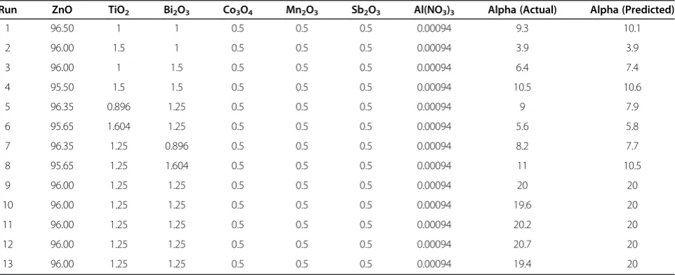
Run ZnO TiO2 Bi2O3 Co3O4 Mn2O3 Sb2O3 Al(NO3)3 Alpha (Actual) Alpha (Predicted)
1 96.50 1 1 0.5 0.5 0.5 0.00094 9.3 10.1
2 96.00 1.5 1 0.5 0.5 0.5 0.00094 3.9 3.9
3 96.00 1 1.5 0.5 0.5 0.5 0.00094 6.4 7.4
4 95.50 1.5 1.5 0.5 0.5 0.5 0.00094 10.5 10.6
5 96.35 0.896 1.25 0.5 0.5 0.5 0.00094 9 7.9
6 95.65 1.604 1.25 0.5 0.5 0.5 0.00094 5.6 5.8
7 96.35 1.25 0.896 0.5 0.5 0.5 0.00094 8.2 7.7
8 95.65 1.25 1.604 0.5 0.5 0.5 0.00094 11 10.5
9 96.00 1.25 1.25 0.5 0.5 0.5 0.00094 20 20
10 96.00 1.25 1.25 0.5 0.5 0.5 0.00094 19.6 20
11 96.00 1.25 1.25 0.5 0.5 0.5 0.00094 20.2 20
12 96.00 1.25 1.25 0.5 0.5 0.5 0.00094 20.7 20
diameter and 0.70 mm thickness at 200 MPa by a uniaxial presser machine. The disks were sintered in a box furnace (CMTS Model HTS 1400) for holding time of 2 h at 1260°C. The heating and cooling rate were 5°C/min [23]. To determine DC current–voltage (I-V), both of the sintered sample surfaces were coated by silver electrodes. The I-V of the samples was measured by Keithley 236 source meter. The samples were scanned with dc voltage from 0 to 100 V in step size of 2.5 V. The alpha was calcu-lated at J1= 0.1 and J2= 1 mA/cm2 by equation (1) as actual responses [6].
α¼ðlogJ2−logJ1Þ=ðlogE2−logE1Þ ð1Þ
The breakdown voltage (Eb) was determined by mea-suring E at J = 0.75 mA/cm2and the leakage current (JL) was determined evaluating J at 0.8Ebwhere J (mA/cm2) is the current density and E is the electrical field (V/mm). To characterize the microstructure, the both surfaces of samples were polished by aluminum oxide powder. Then, they were etched at 160°C under sintering time with heating and cooling rate, 10°C/min. Phase analysis was conducted using XRD (PANalytical, Philips-X’pert Pro PW3040/60) with CuKαsource. The sample were radiated with Ni-filtered CuKαradiation (λ= 1.5428) within the 2θ scan range of 20–80°. Surface morphology and elemental analyses of sintered samples were studied under SEM (JEOL JSM 6400) and VPSEM (LEO 1455) which attached to EDX. The samples was mounted on Al stub using car-bon paint and coated by gold layer. Average grains size of the ZnO in the varistor was evaluated by measuring 100 grains in SEMs images.
Experimental design
The experimental design was carried out by CCD that used Design-Expert software version 8.0.7.1, Stat-Ease Inc., USA [24-26]. CCD is well fixed for fitting a quad-ratic surface that usually works well for optimization process [27-29]. The variables number, level of variables and number of responses are determined as input of ex-perimental design. In this case, the molar ratio of Bi2O3 and TiO2was selected as effective variables in vicinity of their optimum while alpha was the response as output. The CCD transformed the variables and the response to the terms of code values (Table 2) because the units and range of variables were different. The coded values
spaces are ±1 from the center (0.0) and the star points are usually located ‘α’ distance from the center [29,30]. In the design, there N experiment that includes the fac-torial points (2n), the axial points (2n), and the center points Co or replications as the equation N = 2n+ 2n + Cowhich is 13, 4, 4 and 5 respectively. The replications are used to measure experimental error [31]. As a result, the experimental design is presented as a design matrix with‘n’column and‘N’row in Table 1. Where, each co-lumn corresponds to a particular variable, e.g.x1and x2 which arranged in order to increase factor number from left to right. The rows are experiments runs because each one contains the descriptions of an experiment. Additionally, the design constructs a matrix of actual responses that obtained by the experiments.
The RSM description
The RSM develops an adequate functional relationship between input variables and interested responses by low-degree approximation of the polynomial models such as the second degree model (Eq. 2) [32].
Y¼βoþ
Xn
i¼1 βixiþ
Xn
i¼1 βiix2i þ
Xn
i¼1
Xn
j¼iþ1
βijxixjþε
ð2Þ
where Y is the interested response, β0 is the constant
term, βi is the coefficient of the linear terms, βii
repre-sents the coefficient of the quadratic terms,βijis the
co-efficient of the interaction terms while xi are control variables and‘ε’is a random experimental error [31]. For system with two factors, the model is described by equa-tion (3),
Y1i¼β0þβ1x1iþβ11x21iþβ22x22iþβ12x1ix2iþr1i
ð3Þ
whereY1i is the experimental single response,x1and x2 are the coded factors (Table 2), β0is the intercept term, β1andβ2are slopes with respect to each of the two fac-tors, β11 and β22 are curvature terms, and β12 is the interaction term. To estimate the β’s, the fitting process provides the sufficient data by regression tools [33,34]. In the process, the actual responses are fitted to the polynomial models by sequential model sum of squares (SMSS) [33,34]. The SMSS compares the linear, two-factor interaction (2FI), quadratic and cubic models by using the statistical significance of adding new model terms, step by step in increasing order [35]. To select the provisional model, the lack of fit of those models is compared by minimum p-values and PRESS. The other assessments to select
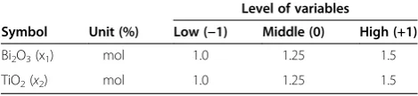
Table 2 The variables and employed levels in the CCD for ZnO low voltage varistor fabrication
Level of variables
Symbol Unit (%) Low (−1) Middle (0) High (+1)
Bi2O3(x1) mol 1.0 1.25 1.5
the best provisional model are maximum adjusted R-squared (RAdj) and predicted R-R-squared (RPred) [36]. The p-value is one of the most important evidences which was used to study significant effect of the para-meters [33]. In addition, the lack-of-fit test diagnoses how well each terms of the full model fit the data that pillared by statistical parameters such as RAdj, RPredand PRESS [36,37]. Therefore, the provisional model with minimum p-value and PRESS and also maximum RAdj, RPredis selected to investigate in details. The details are provided by using analysis of variance (ANOVA) which contains a collection of terms statistical evidences. The ANOVA determines the significance of intercept, linear, interaction and square terms of the provisional model by using minimum p-value. For more evaluation, the normality of residuals, constant error and residual out-lier is checked by various diagnostic plots [38]. The vali-dated model, the relationship between variables and response, is created in coded and actual variables. The model indicates the effect of linear, quadratic and the parameters interactions on the interested response. The effects are presented by estimated coefficients and the related positive and negative signs (+, -). The coeffi-cients are specific weight of the parameters in the model while the signs (+) and (−) operate as synergistic and antagonistic effects on the response [39]. Then the optimization process investigates combination of va-riables levels that produces the maximum response to a surface area simultaneously. Moreover, the model pre-dicts the yield of product in specific condition such as individual standard error, the range of variables and responses. The prediction could be performed by fur-ther experiments.
Results and discussion
Modeling
In the fitting process, the residuals are produced from difference between actual and predicted values. Standard error is a great tool to determine the residuals outlier and also the scope of models prediction [40]. Figure 1 indicates the standard error contour plot of the experi-mental design which displays Bi2O3 versus TiO2 molar ratio. The bright area has relatively low standard error that interested for the modeling and optimization process. However, the darker shading corners represent
higher standard errors which are dangerous to
extrapolation.
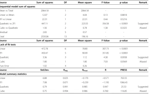
Table 3 indicates that the SMSS compared four models to recommend a proper model [35,36]. As shown, the quadratic model was suggested as the best provisional model. The suggestion based on the lowest standard deviation, p-value and PRESS and the highest RAdj, RPred values. Moreover, the RAdj (0.991) was in reasonable agreement with (<0.20) RPred (0.985) which confirmed the model sufficiency. Therefore, the authors selected the suggested model to investigate in details by using ANOVA.
Table 4 shows the ANOVA of the provisional model which included the useful statistical evidences about the terms (x1, x2, x1x2, x12and x22) in details. As shown, the prob > F of the terms was less than 0.05 which con-firmed the high significance of the terms. Moreover, the model’s F-value was 153.6 that indicated great significance for the model. In addition, the very low value of the model p-value confirmed the significance. Futhermore, R-squared (R) provides a measure of how much variability in the observed response values
can be explained by the experimental factors and their in-teractions. In this study, the R (0.991) indicated that the model was capable of accounting for more than 99.1% of the variability in the responses. The RAdj(0.985) was in rea-sonable agreement with (<0.20) the RPred (0.947) which confirmed the aptness of the model. The pure errors such as experimental errors were minimal as the lack of fit
(0.094) was not significant or the model was fit well. There-fore, ANOVA confirmed the adequacy of the quadratic model that could be used to navigate the design space.
The normality of residuals, constant error and residual outliers were checked by various diagnostic plots. The normal probability plots of the studentized residuals as one of the most important diagnostic plots, was provided
Table 4 Analysis of variance (ANOVA) for response surface quadratic model, MS is mean Square, DF is degree of freedom and SS is sum of squares whilex1andx2introduce in Table 2
Source SS DF MS F-Value p-value (Prob > F) Suggestion
Model 481.5 5 96.3 153.6 < 0.0001 significant
x1 4.6 1 4.6 7.4 0.0299
x2 7.4 1 7.4 11.9 0.0108
x1x2 22.3 1 22.3 35.6 0.0006
x12 298.7 1 298.7 476.4 < 0.0001
x22 205.5 1 205.5 327.7 < 0.0001
Residual 4.4 7 0.6
Lack of Fit 3.4 3 1.1 4.4 0.0938 not significant
Pure Error 1.0 4 0.3 < 0.0001
Cor Total 485.9 12 0.0299
Std.Dev. RAdj RPred R2 PRESS C.V.% Adeq Precision
0.792 0.985 0.947 0.991 25.5 6.284 29.9
Table 3 The sequential model fitting summary for the actual responses which shows statistics conformation of the regression process, DF is degree of freedom
Source Sum of squares DF Mean square F-Value p-value Remark Sequential model sum of squares
Mean vs Total 2064.18 1 2064.18 -
-Linear vs Mean 12.07 2 6.04 0.13 0.8818
2FI vs Linear 22.31 1 22.31 0.44 0.5216
Quadratic vs 2FI 447.11 2 223.55 356.58 < 0.0001 Suggested
Cubic vs Quadratic 1.56 2 0.78 1.38 0.3325 Aliased
Residual 2.83 5 0.57 -
-Total 2550.06 13 196.16 -
-Source Sum of squares DF Mean square F-Value p-value Remark
Lack of fit tests
Linear 472.78 6 78.80 307.73 < 0.0001
2FI 450.47 5 90.09 351.85 < 0.0001
Quadratic 3.36 3 1.12 4.38 0.0938 Suggested
Cubic 1.80 1 1.80 7.03 0.0569 Aliased
Pure Error 1.02 4 0.26 -
-Source Std.Dev. RAdj RPred R PRESS Remark
Model summary statistics
Linear 6.88 0.025 −0.170 −0.571 763.55
2FI 7.08 0.071 −0.239 −1.195 1066.45
Quadratic 0.79 0.991 0.985 0.947 25.53 Suggested
by software default (Figure 2). The plot presents per-centage of normal% probability versus internal studentized residuals. The studentized residual is an important tech-nique in the detection of residuals outliers in regressions [41]. As the plot demonstrates, the residuals followed a normal distribution that implies the points follow a straight line.
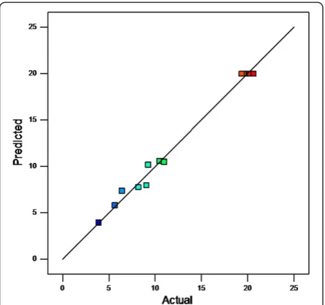
As another diagnosis, Figure 3 illustrates the predicted response values versus the actual response values and detects the values that are not easily predicted by the model. The data points were on the 45 degree line that
means the values were not detected. As a result, the diagnosis of residuals reveals that there is no statistical problem in the model.
The model presentation
The model expresses the relationship between responses of actual variables and the variables themselves. The validated model is presented in actual variables by equation (4),
Y¼−221:67þ211:82x1þ174:00x2
þ37:79x1x2−104:84x21−86:95x 2
2 ð4Þ
where the actual values of the variablesx1andx2were shown in Table 2 and Y is the alpha. As shown, the parameters including linear (x1, x2), quadratic (x12, x22) and interaction (x1x2) affected on the interested res-ponse. The effects are presented by the individual co-efficients and the related signs (+, -) in the model. The coefficients indicate the specific weight of the parame-ters in the model while the signs are synergistic (+) and antagonistic (−) effects of variables on the response (Y).
Table 5 The summary of optimized input variables and obtained maximized alpha% by canonical, graphical, numerical methods and validation value of the photodegradation
Method Bi2O3(%mol) TiO2(%mol) Alpha Canonical (point) 1.195 1.025 15.03
Graphical (area) Area around 1.25 Area around 1.25 20.03
Numerical (prediction) 1.24 1.27 20.03
Validated sample 1.24 1.27 21.6
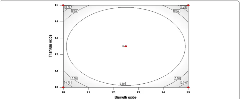
Figure 4The effect of Bi2O3and TiO2on alpha that
simultaneously presented by 3D response surface plot, the maximized alpha was 20.031.
Figure 3Studentized residuals versus predicted values to check the constant error.
The weights determine the importance of the parame-ters roles in the modeling. The model is able to optimize input variables and also approximately predict the response inside of the actual experimental region that confirmed by minimum standard error (Figure 1) [33]. Therefore, the model was used to optimize the molar ratio of Bi2O3 and TiO2 to achieve maximized alpha.
The model optimization
The model is able to optimize the variables by using ca-nonical response and graphical plots. The caca-nonical res-ponses, local optimums, in terms of the code and actual
variables were determined by differentiating the model (Eq. 4) as presented in equations (5 and 6),
∂Y=∂x1
½ x2¼0 ð5Þ
∂Y=∂x2
½ x1¼0 ð6Þ
where the terms were introduced in Table 2. Therefore, the optimum canonical amount of Bi2O3and TiO2were 1.195 and 1.025 respectively. At this optimum, the maxi-mized alpha was 15.03. In fact, the optimization is a kind of the traditional methods, one-variable-at-a-time, be-cause in each case, one of the variables was varied and
Figure 6The EDX of etched optimized sample surfaces.
others were constant. In graphical optimization, the model simultaneously considered the effect of Bi2O3and TiO2on the alpha. Figure 4 presents the three dimen-sion response surface (3D) plot for the synergy between Bi2O3 (1–1.5 mol%) and TiO2 (1–1.5 mol%) which is standard error limitation area (Figure 1). As shown, the alpha increased within 1 to 1.25 mol% Bi2O3and TiO2. However, when the amount of Bi2O3and TiO2was in-creased in excess of the optimum (1.25 mol%), the alpha decreased. Therefore, the optimum was determined in a surface area around 1.25 mol% for the both additives. The maximum alpha was 20.031 at center of the surface which indicated by a flag on top of Figure 4.
The model predicted the maximized alpha in desir-able condition of the additives and standard error which facilitated by default of software numerical op-tion. The desirability is an objective function that uses mathematical methods to find the optimum condition [25]. The range of the function is from zero (outside of the limit area) to one (at the goal). The criteria for this case Bi2O3 (in range), TiO2 (in range), standard error (minimized) and alpha (maximized). The sug-gested solution was Bi2O3 (1.24 mol%), TiO2 (1.27 mol%), standard error (0.35), and alpha 20.03. The de-sirability of the solution was 0.981 which is close to 100% (at the goal). The solution was performed to confirm the prediction by validated experiment. The validated alpha was determined 21.6 which was quite close to the predicted alpha (20.03). Table 5 illustrated a summary of optimized molar ratios of Bi2O3 and
TiO2 and also the related maximized alpha which
obtained by canonical, graphical and numerical model optimization method.
The validated varistor
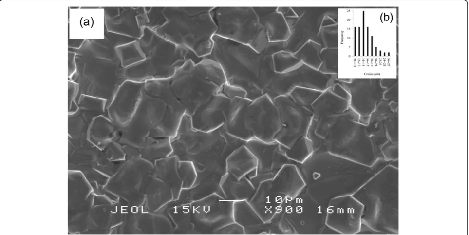
The validated sample was characterized as final varistor for this optimization process. Figure 5 demonstrates the SEM morphology of the sintered ceramic microstructure of the varistor. Figure 5a indicates the great homogeneity of ZnO grain size. The average grain size was 15μm (Figure 5b).
Figure 6 illustrates EDX spectra of a limited area of the etched varistor surfaces composition. As shown all addi-tives particular Bi (1.0 weight%) and Ti (1.17 weight%) were detected in the selected area after sintering process at 1260°C.
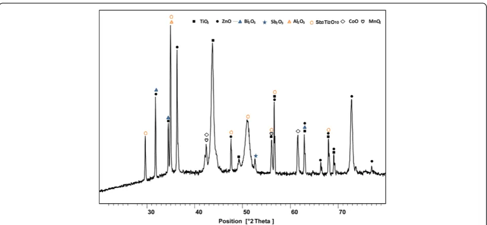
Figure 7 shows the XRD pattern of the optimized sam-ple which presented three phase of ZnO, spinel and metal
Figure 8E-J characteristic curves of the optimized samples for first to fourth measurments.
oxide of additives. The composites were including ZnO (00-005-0664), Bi2O3(00-002-0988), TiO2(01-072-0020), MnO2 (00-003-1041), CoO (00-048-1719), Sb2O3 (01-075-1567), Al2O3(00-004-0879) and Sb3Ti2O10 (00-028-0103). The number that mentioned in parenthesis are XRD reference code.
The electrical properties of the varistor were basis of I-V characteristic measurement that shows breakdown voltage was 98 V/mm with non-linear coefficient 21.6. The leakage current was 0.013 mA/cm2. The stability of the varistor was measured by alpha recovery after re-moving the over voltage (Figure 8). As shown the stabi-lity was quit significant after fourth over voltage.
Conclusions
This work reports modeling and optimization of the molar ratio of Bi2O3 and TiO2 by RSM. The fabrication was designed by CCD using two variables and a response. To obtain actual responses, the design was performed in laboratory by conventional fabrication methods. The ac-tual responses were fitted into a quadratic model. The model was validated by ANOVA which provided evi-dences such as high F-value (153.6), very low p-value (<0.0001), Radj(0.985) and RPred(0.947). The results of the validation showed the model was significant. The model tracked the optimum of the designed additives by using 3D plots. In the optimum condition, the molars ratio of Bi2O3 and TiO2 were around 1.25 that maximized the alpha value at 20. Moreover, the model suggested a solu-tion to predict the optimum amount of the additives. In this case, the condition of the solution included standard error of 0.35, Bi2O3 of 1.24, TiO2 of 1.27 and alpha of 20.03. The solution was tested by further experiments. As the validation test showed, the obtained value of the alpha (21.6) was very close to the predicted value (20.03). There-fore, RSM was succeeded in modeling of the additives in fabrication of zinc oxide based low voltage varistor to achieve maximum alpha.
Competing interests
The authors declare that they have no competing interests.
Authors’contributions
YA carried out the catalyst design and ligand screening studies. YA, SNA-T, NMM-S and NMS carried out the synthesis, purification and characterization of the compounds. YA carried out the computational experiments. AZ, RSA and KAM conceived of the study, and participated in its design and coordination and helped to draft the manuscript. All authors read and approved the final manuscript.
Acknowledgements
The author would like to express acknowledgement to Ministry of Higher Education Malaysia for granting this project under Research University Grant Scheme (RUGS) of Project No. 05-02-12-1878. The authors wish to thank Dr Pedram Lalbakhsh for polishing and proofreading the manuscript.
Author details
1
Material Synthesis and Characterization Laboratory, Institute of Advanced Technology, Universiti Putra Malaysia, 43400 UPM, Serdang, Selangor,
Malaysia.2Department of Physics, Faculty Science, Universiti Putra Malaysia,
43400 UPM, Serdang, Selangor, Malaysia.
Received: 19 May 2013 Accepted: 6 August 2013 Published: 10 August 2013
References
1. Ramírez M, Bueno P, Ribeiro W, Varela J, Bonett D, Villa J, Márquez M, Rojo C:The failure analyses on ZnO varistors used in high tension devices.J Mater Sci2005,40:5591–5596.
2. Ramirez M, Bassi W, Bueno P, Longo E, Varela J:Comparative degradation of ZnO-and SnO2-based polycrystalline non-ohmic devices by current pulse stress.J Phys D Appl Phys2008,41:122002–122002.
3. Ramírez MA, Bassi W, Parra R, Bueno PR, Longo E, Varela JA:Comparative electrical behavior at low and high current of SnO2and ZnO based
varistors.J Am Ceram Soc2008,91:2402–2404.
4. Levinson L, Philipp H:Zinc oxide varistors–a review.Am Ceram Soc Bull 1986,65:639.
5. Eda K:Zinc oxide varistors.IEEE Electr Insul Mag2002,5:28–30. 6. Bernik S, Zupancic P, Kolar D:Influence of Bi2O3/TiO2/Sb2O3and Cr2O3
doping on low-voltage varistor ceramics.J Eur Ceram Soc1999, 19:709–713.
7. Suzuki H, Bradt R:Grain growth of ZnO in ZnO-Bi2O3ceramics with TiO2
addition.J Am Ceram Soc1995,78:1354–1360.
8. Clarke DR:Varistor ceramics.J Am Ceram Soc1999,82:485–502. 9. Pillai SC, Kelly JM, McCormack DE, O'Brien P, Ramesh R:The effect of
processing conditions on varistors prepared from nanocrystalline ZnO. J Mater Chem2003,13:2586–2590.
10. Elfwing M, Österlund R, Olsson E:Differences in wetting characteristics of Bi2O3polymorphs in ZnO varistor materials.J Am Ceram Soc2000,
83:2311–2314.
11. Lao Y-W, Kuo S-T, Tuan W-H:Effect of Bi2O3and Sb2O3on the grain
size distribution of ZnO.J Electroceram2007,19:187–194. 12. Peiteado M, Fernández Lozano JF, Caballero AC:Varistors based in the
ZnO-Bi2O3system: microstructure control and properties.J Eur Ceram Soc
2007,27:3867–3872.
13. Peiteado M, De la Rubia M, Velasco M, Valle F, Caballero A:Bi2O3
vaporization from ZnO-based varistors.J Eur Ceram Soc2005, 25:1675–1680.
14. Metz R, Delalu H, Vignalou J, Achard N, Elkhatib M:Electrical properties of varistors in relation to their true bismuth composition after sintering. Mater Chem Phys2000,63:157–162.
15. Wong J:Sintering and varistor characteristics of ZnO Bi2O3ceramics.
J Appl Phys1980,51:4453–4459.
16. Yilmaz S, Ercenk E, Toplan HO, Gunay V:Grain growth kinetic in x TiO 2–6 wt.% Bi 2 O 3–(94−x) ZnO (x = 0, 2, 4) ceramic system.J Mater Sci2007, 42:5188–5195.
17. Toplan HÖ, KarakaşY:Processing and phase evolution in low voltage varistor prepared by chemical processing.Ceram Int2001, 27:761–765.
18. Yan MF, Heuer AH:Additives and interfaces in electronic ceramics.Columbus, OH: Amer Ceramic Society; 1983.
19. Peigney A, Andrianjatovo H, Legros R, Rousset A:Influence of chemical composition on sintering of bismuth-titanium-doped zinc oxide. J Mater Sci1992,27:2397–2405.
20. Bernik S, Daneu N, Rečnik A:Inversion boundary induced grain growth in TiO2or Sb2O3doped ZnO-based varistor ceramics.J Eur Ceram Soc2004,
24:3703–3708.
21. Montgomery DC:Design and analysis of experiments.New York: John Wiley & Sons Inc; 2008.
22. Khuri AI, Cornell JA:Response surfaces: designs and analyses.New York: CRC; 1996.
23. Bernik S:Microstructural and electrical characteristics of ZnO based varistor ceramics with varying TiO2/Bi2O3ratio. InAdvances in science and
technology; 1999:151–158.
24. Williges RC, Clark C:Response surface methodology design variants useful in human performance research, Illinois Univ Savoy Aviation Research Lab.; 1971. 25. Myers RH, Anderson-Cook CM:Response surface methodology: process and
26. Clark C, Williges RC:Response surface methodology design variants useful in human performance research, DTIC Document, New York; 1971. 27. Deming S:Quality by design-part 5.Chemtech1990,20:118–120. 28. Hader R, Park SH:Slope-rotatable central composite designs.
Technometrics1978,20:413–417.
29. Palasota JA, Deming SN:Central composite experimental designs: applied to chemical systems.J Chem Educ1992,69:560. 30. Rubin IB, Mitchell TJ, Goldstein G:Program of statistical designs for
optimizing specific transfer ribonucleic acid assay conditions. Anal Chem1971,43:717–721.
31. BaşD, Boyacı İH:Modeling and optimization I: usability of response surface methodology.J Food Eng2007,78:836–845.
32. Khuri AI, Mukhopadhyay S:Response surface methodology. Wiley Interdiscip Rev Comput Stat2010,2:128–149.
33. Anderson MJ, Whitcomb PJ:RSM simplified: optimizing processes using response surface methods for design of experiments.Virginia: Productivity Pr; 2005.
34. Oehlert GW:A first course in design and analysis of experiments.New York: WH Freeman; 2000.
35. Deming S:Quality by design-part 3.Chemtech1989,19:249–255. 36. Whitcomb PJ, Anderson MJ:RSM simplified: optimizing processes using
response surface methods for design of experiments.New York: Productivity Press; 2004.
37. Allen DM:The relationship between variable selection and data agumentation and a method for prediction.Technometrics1974, 16:125–127.
38. Stuart A, Ord JK:Kendall’s advanced theory of statistics: vol 1. Distribution theory.London: Arnold; 1994.
39. Abdollahi Y, Zakaria A, Abdullah AH, Masoumi HRF, Jahangirian H, Shameli K, Rezayi M, Banerjee S, Abdollahi T:Semi-empirical study of ortho-cresol photo degradation in manganese-doped zinc oxide nanoparticles suspensions.Chem Cent J2012,6:1–8.
40. Box GEP, Wilson K:On the experimental attainment of optimum conditions.J Roy Stat Soc B1951,13:1–45.
41. Stuart A, Ord JK, Arnold S:Kendall’s advanced theory of statistics: vol 2A. Classical inference and the linear model.London: Arnold; 1999.
doi:10.1186/1752-153X-7-137
Cite this article as:Abdollahiet al.:Optimizing Bi2O3and TiO2to
achieve the maximum non-linear electrical property of ZnO low voltage varistor.Chemistry Central Journal20137:137.
Open access provides opportunities to our colleagues in other parts of the globe, by allowing
anyone to view the content free of charge.
Publish with
Chemistry
Central and every
scientist can read your work free of charge
W. Jeffery Hurst, The Hershey Company.
available free of charge to the entire scientific community peer reviewed and published immediately upon acceptance cited in PubMed and archived on PubMed Central yours you keep the copyright
Submit your manuscript here: