R E S E A R C H
Open Access
Two regularization methods for a class of
inverse boundary value problems of elliptic
type
Abdallah Bouzitouna
1, Nadjib Boussetila
2*and Faouzia Rebbani
1*Correspondence:
2Department of Mathematics, 8 Mai
1945 Guelma University, P.O. Box 401, Guelma, 24000, Algeria Full list of author information is available at the end of the article
Abstract
This paper deals with the problem of determining an unknown boundary condition
u(0) in the boundary value problemuyy(y) –Au(y) = 0,u(0) =f,u(+∞) = 0, with the aid
of an extra measurement at an internal point. It is well known that such a problem is severely ill-posed,i.e., the solution does not depend continuously on the data. In order to overcome the instability of the ill-posed problem, we propose two regularization procedures: the first method is based on the spectral truncation, and the second is a version of the Kozlov-Maz’ya iteration method. Finally, some other convergence results including some explicit convergence rates are also established undera prioribound assumptions on the exact solution.
MSC: 35R25; 65J20; 35J25
Keywords: ill-posed problems; elliptic problems; cut-off spectral regularization; iterative regularization
1 Formulation of the problem
Throughout this paper,Hdenotes a complex separable Hilbert space endowed with the inner product (·,·) and the norm · ,L(H) stands for the Banach algebra of bounded linear operators onH.
LetA:D(A)⊂H→Hbe a positive, self-adjoint operator with compact resolvent, so thatAhas an orthonormal basis of eigenvectors (φn)⊂Hwith real eigenvalues (λn)⊂R+, i.e.,
Aφn=λnφn, n∈N∗, (φi,φj) =δij=
⎧ ⎨ ⎩
ifi=j,
ifi=j,
<ν≤λ≤λ≤λ≤ · · ·, lim
n→∞λn=∞,
∀h∈H, h=
∞
n=
hnφn, hn= (h,φn).
In this paper, we are interested in the following inverse boundary value problem: find (u(y),u()) satisfying
⎧ ⎨ ⎩
uyy–Au= , <y<∞,
u() =f, u(+∞) = , (.)
wheref is the unknown boundary condition to be determined from the interior data
u(b) =g∈H, <b<∞. (.)
This problem is an abstract version of an inverse boundary value problem, which general-izes inverse problems for second-order elliptic partial differential equations in a cylindrical domain, for example we mention the following problem.
Example . An example of (.) is the boundary value problem for the Laplace equation in the strip (,π)×(,∞), where the operatorAis given by
A= –∂
∂x, D(A) =H
(,π)∩H(,π)⊂H=L(,π),
which takes the form
⎧ ⎪ ⎪ ⎪ ⎪ ⎪ ⎨ ⎪ ⎪ ⎪ ⎪ ⎪ ⎩
uyy(x,y) +uxx(x,y) = , x∈(,π),y∈(, +∞),
u(,y) =u(π,y) = , y∈(, +∞),
u(x, ) =f(x), u(x, +∞) = , x∈[,π],
u(x,y=b) =g(x), x∈[,π].
To our knowledge, there are few papers devoted to this class of problems in the abstract setting, except for [, ]. In [], the author studied a similar problem posed on a bounded interval. In this study, the algebraic invertibility of the inverse problem was established. However, the regularization aspect was not investigated.
We note here that this inverse problem was studied by Levine and Vessella [], where the authors considered the problem of recoveringu() from the experimental datag, . . . ,gn
associated to the internal measurementsu(b), . . . ,u(bn), in which the temperature is
mea-sured at various depths <b <· · ·<bn as approximate functions g, . . . ,gn∈H such
that
n
i=
piu(bi) –gi≤ε,
wherep, . . . ,pnare positive weights with
n
i=pi= andεdenotes the level noisy.
The regularizing strategy employed in [] is essentially based on the Tikhonov regular-ization and the conditional stability estimateuy() ≤Efor somea prioriconstantE.
In practice, the use ofN-measurements or the average of a series of measurements is an expensive operation, and sometimes unrealizable. Moreover, the numerical implemen-tation of the stabilized solutions by the Tikhonov regularization method for this class of problems will be a very complex task.
2 Preliminaries and basic results
In this section we present the notation and the functional setting which will be used in this paper and prepare some material which will be used in our analysis.
2.1 Notation
We denote byC(H) the set of all closed linear operators densely defined inH. The do-main, range and kernel of a linear operatorB∈C(H) are denoted asD(B),R(B) andN(B); the symbolsρ(B),σ(B) andσp(B) are used for the resolvent set, spectrum and point
spec-trum ofB, respectively. IfV is a closed subspace ofH, we denote byV the orthogonal
projection fromHtoV.
For the ease of reading, we summarize some well-known facts in spectral theory.
2.2 Spectral theorem and properties
By the spectral theorem, for each strictly positive self-adjoint operatorB,
B:D(B)⊂H→H, D(B) =H, B=B∗ and (Bu,u)≥γu, ∀u∈D(B) (γ > ),
there is a unique right continuous family{Eλ,λ∈[γ,∞[} ⊂L(H) of orthogonal projection
operators such thatB= γ∞λdEλwith
D(B) =
v∈H: ∞
γ
λd(Eλv,v) <∞
.
Theorem . [, Theorem , XII.., pp.-] Let{Eλ,λ≥γ > }be the spectral
resolution of the identity associated to B,and letbe a complex Borel function defined E-almost everywhere on the real axis.Then(B)is a closed operator with dense domain. Moreover,
(i) D((B)) :={h∈H: γ∞|(λ)|d(E
λv,v) <∞}, (ii) ((B)h,y) = γ∞(λ)d(Eλh,y),h∈D((B)),y∈H, (iii) (B)h= ∞
γ |(λ)|
d(E
λh,h),h∈D((B)),
(iv) (B)∗=(B).In particular,ifis a real Borel function,then(B)is self-adjoint.
We denote byS(y) =e–y
√
A=+∞
n=e–y
√
λn(·,φ
n)φn∈L(H),y≥, theC-semigroup gen-erated by –√A. Some basic properties ofS(y) are listed in the following theorem.
Theorem . (see [], Chapter , Theorem ., p.) For this family of operators, we have:
. S(y) ≤,∀y≥;
. the functiony−→S(y),y> ,is analytic;
. for every realr≥andy> ,the operatorS(y)∈L(H,D(Ar/));
. for every integerk≥andy> ,S(k)(y)=Ak/S(y) ≤c(k)y–k; . for everyh∈D(Ar/),r≥,we haveS(t)Ar/h=Ar/S(y)h.
Proof Letφy: [, +∞[→R,s−→φy(s) =e–ys. Then, by virtue of (iv) of Theorem ., we
can writeS(y)∗=φy(A) =φy(A) =e–y
√
A=S(y).
Leth∈N(S(y)),y> , thenS(y)h= , which implies thatS(y)S(y)h=S(t+t)h= , y≥. Using analyticity, we obtain thatS(y)h= ,y≥. Strong continuity at now gives h= . This shows thatN(S(y)) ={}.
Thanks to
RS(y)
=NS(y) ⊥
={}⊥=H,
we conclude thatR(S(y)) is dense inH.
Remark . Fory=b, this theorem ensures thatS(b) is self-adjoint and one-to-one op-erator with dense rangeR(S(b)). Then we can define its inverseS(b)–=eb√A, which is an
unbounded self-adjoint strictly positive definite operator inHwith dense domain
DS(b)–=RS(b)=
h∈H:eb
√
Ah=
+∞
n= eb
√
λn(h,φ
n)
< +∞
.
Let us consider the following problem: forξ∈H findv∈C(], +∞[;H)∩C([, +∞[; H)∩C(], +∞[;D(A)) such that
v(y) +√Au(y) = , <y< +∞,v() =ξ. (.)
Theorem .[, Theorem ., p.] For anyξ∈H,problem(.)has a unique solution,
given by
v(y) =S(y)ξ=
∞
n=
e–y√λn(ξ,φ
n)φn. (.)
Moreover,for all integer k≥,v∈C∞(], +∞[;D(Ak/)).If,in addition,ξ∈D(Aj/),then v∈C([, +∞[;D(Aj/))∩Cj([, +∞[;H)and
∀k,j∈N, d (k+j)
dy v(y)
=Ak/u(y)(j)≤c(k) yk A
j/ξ.
On the other hand, Theorem . provides smoothness results with respect to y: v∈ C∞(], +∞[;H)∩Cj([, +∞[;H) wheneverξ∈D(Aj/),j∈N. Under this same hypothesis, we also have smoothness in space:v∈C([, +∞[;D(Aj/))∩Cj–k([, +∞[;D(Ak/)),k≤j.
Here we recall a crucial theorem in the analysis of the inverse problems.
Theorem .[, Generalized Picard theorem, p.] Let B:D(B)⊂H→H be a self-adjoint operator and the Hilbert space H,and let Eμbe its spectral resolution of unity.Let θ ∈C(R,R)and Z(θ) :={t∈R:θ(t) = }.We suppose that the set Z(θ)either is empty or contains isolated point only.Then the vectorial equation
is solvable if and only if
R
θ(λ)–d|Eλψ|<∞.
Moreover,
Nθ(B)={} ⇐⇒ σp(B)∩Z(θ) =∅.
On the basis{φn}, we introduce the Hilbert scale (Hs)s∈R(resp. (Es)s∈R) induced by
√ A as follows:
Hs=
h∈H:
∞
n=
λn
s
(h,ϕn)< +∞
,
Es=
h∈H:
∞
n=
ebs√λn(h,ϕ
n)< +∞
.
2.3 Non-expansive operators
Definition . A linear operatorM∈L(H) is called non-expansive if
M ≤.
Theorem . [, Theorem .] Let M∈L(H)be a positive, self-adjoint operator with M ≤.Putting V=N(M)and V=N(I–M),we have
s– lim
n→+∞M
n=
V, s– lim
n→+∞(I–M)
n= V,
i.e.,
∀h∈H, lim
n→+∞M
nh=
Vh, lim
n→+∞(I–M)
nh= Vh.
For more details concerning the theory of non-expansive operators, we refer to Kras-nosel’skiiet al.[, p.].
Let use consider the operator equation
Sϕ= (I–M)ϕ=ψ (.)
for non-expansive operatorsM.
Theorem . Let M be a linear self-adjoint,positive and non-expansive operator on H. Letψˆ ∈H be such that equation(.)has a solutionϕˆ.Ifis not an eigenvalue of M,i.e., (I–M)is injective(V=N(I–M) ={}),then the successive approximations
ϕn+=Mϕn+ψˆ, n= , , , . . . ,
Proof From the hypothesis and by virtue of Theorem ., we have
∀ϕ∈H, Mnϕ→Vϕ={}ϕ= . (.)
By induction with respect ton, it is easily seen thatϕnhas the explicit form
ϕn=Mnϕ+
n–
j= Mjψˆ
=Mnϕ+
I–Mn(I–M)–ψˆ
=Mnϕ+
I–Mnϕˆ,
and (.) allows us to conclude that
ˆ
ϕ–ϕn=Mn(ϕ–ϕˆ)→, n→ ∞. (.)
Remark . In many situations, some boundary value problems for partial differential equations which are ill-posed can be reduced to Fredholm operator equations of the first kind of the form Bϕ =ψ, whereBis compact, positive, and self-adjoint operator in a Hilbert spaceH. This equation can be rewritten in the following way:
ϕ= (I–ωB)ϕ+ωψ=Lϕ+ωψ,
whereL= (I–ωB), andωis a positive parameter satisfyingω<
B. It is easily seen that the
operatorLis non-expansive and is not an eigenvalue ofL. It follows from Theorem . that the sequence{ϕn}∞n=converges and (I–ωB)nζ→ for everyζ∈Hasn→ ∞.
3 Ill-posedness and stabilization of the inverse boundary value problem
3.1 Cauchy problem with Dirichlet conditions
Consider the following well-posed boundary value problem:
⎧ ⎪ ⎪ ⎨ ⎪ ⎪ ⎩
vyy–Av= , <y<∞,
v() =ξ,
v(+∞) = ,
(.)
whereξ is anH-valued function.
Definition .[, p.]
• A functionv: [, +∞[→His called a generalized solution to equation(.)if
v∈Eg=C([, +∞[;H)∩C(], +∞[;H)∩C([, +∞[;H–), and for ally∈], +∞[,
u(y)∈D(A)and obeys equation(.)on the same interval], +∞[. • A functionv: [, +∞[→His called a classical solution to equation(.)if
Theorem . Problem(.)admits a unique generalized(resp.classical)solution if and only ifξ∈H(resp.ξ∈H).
Proof By using the Fourier expansion and the given Dirichlet boundary conditions
v(y) = +∞
n=
vn(y)φn,
v() = +∞
n=
vn()φn=ξ=
+∞
n=
ξnφn,
v(+∞) = +∞
n=
vn(+∞)φn= ,
we obtain ⎧ ⎪ ⎪ ⎨ ⎪ ⎪ ⎩
vn–λnvn(y) = , <y<∞,
vn() =ξn,
vn(+∞) = .
(.)
This differential equation admits two linearly independent fundamental solutions
ϕn+(y) =e+y√λn, ϕ–
n(y) =e–y
√
λn.
Thus, its general solution can be written as
vn(y) =c+ne
+y√λn+c–
ne
–y√λn, c+
n,c
–
n∈R.
Applyingvn(+∞) = andvn() =ξnyieldsc+n= andc–n=ξn. Finally, the solution of (.)
is
v(y) =S(y)ξ=e–y
√
Aξ=
+∞
n= e–y√λnξ
nφn, ξn= (ξ,φn). (.)
Remark . It is easy to check that the expression (.) solves the problem
u(y) +√Au(y) = , y∈], +∞[, u() =ξ.
Ifξ∈H (resp.ξ∈H), by virtue of Theorem . and Remark ., we easily check the inclusionv∈Eg(resp.v∈Ec) andv(y)∈D(A) fory∈], +∞[.
3.2 Inverse boundary value problem
Our inverse problem is to determinev() =f from the supplementary conditionv(b) =g, then we get
v(b) = +∞
n= e–b√λnf
nφn=g=
+∞
n=
We define
K=S(b) :H→H, h−→Kh= +∞
n=
e–b√λnh
nφn. (.)
The operator equation (.) is the main instrument in investigating problem (.). More precisely, we want to study the following properties:
. Injectivity ofK(identifiability);
. Continuity ofKand the existence of its inverse (stability); . The range ofK.
It is easy to see thatK is a linear compact self-adjoint operator with the singular values (σk=e–b
√
λk)+∞
k=, and by virtue of Remark ., we have
. N(K) ={},
. R(K) =
h∈H:eb√Ah=
+∞
n=
eb√λn(h,φ
n)< +∞
,
. R(K) =H.
Now, to conclude the solvability of problem (.) it is enough to apply Theorem ..
Corollary . The inverse problem(.)is uniquely solvable if and only if
u(b) =g∈R(K) =
h∈H: +∞
n=
eb√λn(h,φ
n)
< +∞
. (.)
In this case,we have
f =u() =K–g= +∞
n= eb√λng
nφn. (.)
In other words, the solutionf of the inverse problem is obtained from the datagvia the unbounded operatorL=K–defined on functionsgin the subspace
D(L) =
g∈H: +∞
n=
eb√λn(g,φn)< +∞,g
n= (g,φn)
.
Corollary . Problem(.)-(.)admits a unique solution u∈C([, +∞[;H)if and only if
u()∈H ⇐⇒ g∈R(K) =
h∈H: +∞
n=
eb√λn(h,φ
n)
< +∞
.
In this case,we have
u(y) =e(b–y)
√
Ag=
+∞
n=
e(b–y)√λng
From this representation, we see that:
• u(y)is stable in the interval[b, +∞[(supy∈[b,+∞[u(y) ≤ g); • uis unstable in[,b[. This follows from the high-frequencyωn=e(b–y)
√
λn→+∞,
n→+∞.
3.3 Regularization by truncation method and error estimates
A natural way to stabilize the problem is to eliminate all the components of largenfrom the solution and instead consider (.) only forn≤N.
Definition . ForN> , the regularized solution of problem (.)-(.) is given by
fN=
n≤N
eb√λng
nφn, gn= (g,φn), (.)
uN(y) =
n≤N
e(b–y)√λng
nφn, gn= (g,φn). (.)
Remark . If the parameterNis large,fN is close to the exact solutionf. On the other
hand, if the parameterNis fixed,fN is bounded. So, the positive integerNplays the role
of regularization parameter.
Remark . In view of
u(y) –uN(y)=S(y)(f –fN)≤(f–fN) ⇒ u–uN∞≤(f –fN),
and ifg∈E,i.e.,∞n=eb√λn|(g,φ
n)|<∞, then
f–fN →, N→ ∞,
implies
u–uN∞= sup y∈[,+∞[
u(y) –uN(y)→, N→ ∞.
Since the datagare based on (physical) observations and are not known with complete accuracy, we assume thatg andgδ satisfyg–gδ ≤δ, wheregδ denotes the measured
data andδdenotes the level noisy. Let (fδ
N,u δ
N) denote the regularized solution of problem (.), (.) with measured datagδ:
fNδ=
n≤N
eb
√
λngδ
nφn, gnδ=
gδ,φn
, (.)
uδN(y) =
n≤N
e(b–y)√λngδ
nφn, gnδ=
gδ,φn
. (.)
As usual, in order to obtain convergence rate, we assume that there exists ana priori bound for problem (.)
Ar/f≤E< +∞ ⇐⇒ +∞
n=
λrneb√λn|g
n|≤E, (.)
Remark . For given two exact conditionsgandg, letf,Nandf,Nbe the corresponding
regularized solutions, respectively. Then
f,N–f,N=
n≤N
eb
√
λn(g –g)k
≤eb√λNg
–g. (.)
The main theorem of this method is as follows.
Theorem . Let fδ
N be the regularized solution given by(.),and let f be the exact
so-lution given by(.).IfAr/f ≤E,r> and if we choose√λ
N≈ θblog(δ), <θ< ,then
we have the error bound
f –fNδ≤
b
θ
r
log(/δ) r
E+δ–θ. (.)
Proof From direct computations, we have
=fN–fNδ≤eb
√
λNg–gδ≤eb√λNδ,
=f –fN=
+∞
n=N+ eb√λn|g
n|
= +∞
n=N+ √ λn r λn r
eb√λn|g
n|
≤√
λN+r +∞
n=N+
λn
r
eb√λn|g
n|
≤ √ λN r
E.
Using the triangle inequality
f –fNδ≤ f–fN+fN–fNδ=+,
we obtain
f –fNδ≤
√
λN
r
E+eb√λNδ. (.)
By choosing√λN =θblog(δ), <θ< , we obtain
f –fδ N≤
b
θ
r
log(/δ)
r
E+δ–θ.
Finally, from (.) and (.), we deduce the following corollary.
Corollary . Let uδ
N be the regularized solution given by(.),and let u be the exact
solution given by(.).IfAr/f ≤E,r> and if we choose√λ
N=θblog(δ), <θ< ,then
we have the error bound
u–uδN∞= sup
y∈[,+∞[
u(y) –uδN(y)≤f –fNδ≤
b
θ
r
log(/δ) r
4 Regularization by the Kozlov-Maz’ya iteration method and error estimates In [, ] Kozlov and Maz’ya proposed an alternating iterative method to solve boundary value problems for general strongly elliptic and formally self-adjoint systems. After that, the idea of this method has been successfully used for solving various classes of ill-posed (elliptic, parabolic and hyperbolic) problems; see,e.g., [–].
In this section we extend this method to our ill-posed problem.
4.1 Description of the method
The iterative algorithm for solving the inverse problem (.)-(.) starts by lettingf∈H be arbitrary. The first approximationu(y) is the solution to the direct problem
⎧ ⎪ ⎪ ⎨ ⎪ ⎪ ⎩
u
yy–Au= , <y<∞,
u() =f,
u(+∞) = .
(.)
If the pair (uk,f
k) has been constructed, let
(P)k+: fk+=fk–ω
uk(b) –f, (.)
whereωis such that
<ω< K=e
b√λ, K=sup
n
e–b√λn=e–b√λ< .
Finally, we getuk+by solving the problem
⎧ ⎪ ⎪ ⎨ ⎪ ⎪ ⎩
ukyy+–Auk+= , <y<∞,
uk+() =f
k+,
uk+(+∞) = .
(.)
We setG= (I–ωK). If we iterate backwards in (P)k+, we obtain
fk=Gkf+ω
k–
i=
Gig=Gkf+
I–GkK–g=Gkf+f –Gkf. (.)
This implies that
fk–f=Gk(f–f), uk(y) –u(y) =S(y)Gk(f–f). (.)
Proposition . The operator G= (I–ωK)is self-adjoint and non-expansive on H. More-over,it has notas eigenvalue.
Proof The self-adjointness follows from the definition ofG(see Theorem .). Since the inequality < –ωe–b√λ< forλ∈σ(A), we haveσ
p(G)⊂], [, then is not an eigenvalue
In general, the exact solutionu() =f ∈H is required to satisfy the so-called source condition; otherwise, the convergence of the regularization method approximating the problem can be arbitrarily slow. Since our problem is exponentially ill-posed (the eigen-valuessn=e–b
√
λnofKconverge exponentially to ), it is well known in this case [, ]
that the best choice to accelerate the convergence of the regularization method is to use logarithmic-type source conditions,i.e.,
(f–f) =β(ωK)ξ, ξ∈H,ξ ≤E, (.)
where
β(t) = ⎧ ⎨ ⎩
ln(et)–β, <t≤,
, t= ,
withβ> .
Remark .[, p.] The logarithmic source conditionζ = (f–f)∈R(β(ωK)) is
equiv-alent to the inclusionζ∈R(A–β/) =D(Aβ/).
Proof The proof is based on the following equivalence:
∞
k=
ln
e
ω
+λn
β
< +∞ ⇐⇒
∞
k=
(λn)β< +∞.
Lemma .[, Appendix, Lemma A.] Letβ> and k∈N,k≥.Then the real-valued functionτ(t) = ( –t)kln(e
t)
–βdefined on[, ]satisfies
τ(t)≤Cln(k)–β. (.)
Remark . Letk∈N∗. Then the real-valued function(t) = – ( –t)kdefined on [, ]
satisfies
(t)≤kt. (.)
Proof Using the mean value theorem, we can write
(t) –() = (t– )(ˆt), <ˆt<t, then
(t) =tk( –ˆt)k–≤kt.
Let us consider the following real-valued functions:
Q(λ) = –ωe–b
√
λkln
e
ωe–b√λ
–β
, λ∈[λ, +∞[,
P(λ) =ω k–
i=
–ωe–b
√
λi
=ω – ( –ωe
–b√λ)k
Using the change of variablest=ϑ(λ) =ωe–b√λ, we obtain
ˆ
Q(t) =Qϑ–(t)= ( –t)kln
e t
–β
, t∈[, ],
ˆ
P(t) =Pϑ–(t)= ⎧ ⎨ ⎩
ω–(–tt)k, t∈], ],
ωk, t= .
Now we are in a position to state the main result of this method.
Theorem . Let g∈Eandωsatisfy <ω<eb√λ,let f
be an arbitrary element for the iterative procedure suggested above,and let ukbe the kth approximate solution.Then we
have
sup
y∈[,+∞[
u(y) –uk(y)→, k→ ∞. (.)
Moreover,if(f–f)∈Hβ(β> ),i.e., (f–f) =β(ωK)ξ,ξ∈H,ξ ≤E,then the rate of
convergence of the method is given by
sup
y∈[,+∞[
u(y) –uk(y)≤CE
ln(k)
β
, k≥. (.)
Proof By virtue of Proposition . and Theorem ., it follows immediately
sup
y∈[,+∞[
u(y) –uk(y)≤Gk(f–f)→, k→ ∞.
We have
u(y) –uk(y) =S(y)Gk(f–f)
≤Gk(f–f)
=
∞
n=
Q(λn)(ξ,φn)
≤sup
t∈[,] ˆ Q(t)
ξ≤
sup
t∈[,] ˆ Q(t)
E,
and by virtue of Lemma . (estimate (.)), we conclude the desired estimate.
Theorem . Let g∈Eandωsatisfy <ω<eb√λ,let f
be an arbitrary element for the iterative procedure suggested above,and let uk(resp.uδ
k)be the kth approximate solution
for the exact data g (resp.for the inexact data gδ)such thatg–gδ ≤δ.Then,under
condition(.),the following inequality holds:
sup
y∈[,+∞[
u(y) –ukδ(y)≤CE
ln(k)
β
+ε(k)δ,
Proof Using (.) and the triangle inequality, we can write
fk=Gkf+ω
k–
i=
Gig,uk(y) =S(y)fk, (.)
fδk=Gkf+ω
k–
i= Gigδ,uδ
k(y) =S(y)fδk, (.)
u(y) –ukδ(y)=u(y) –uk(y)
+uk(y) –ukδ(y)≤+,
where
=u(y) –uk(y)≤u(y) –uk(y)∞≤CE
ln(k)
β
, k≥, (.)
and
=uk(y) –uδk(y)=S(y)
fk–fδk= ωS(y)
k–
i=
Gig–gδ
≤ω k–
i=
Gig–gδ
≤ ω k– i= Gi δ=ˆ.
By using inequality (.), the quantityˆcan be estimated as follows:
ˆ
≤ωkδ. (.)
Combining (.) and (.) and taking the supremum with respect to y∈[, +∞[ of u(y) –uk
δ(y), we obtain the desired bound.
Remark . Choosingk=k(δ) such thatωkδ→+∞asδ→, we obtain
sup
y∈[,+∞[
uk(y) –ukδ(y)→ ask→+∞.
5 Numerical results
In this section we give a two-dimensional numerical test to show the feasibility and effi-ciency of the proposed methods. Numerical experiments were carried out using MATLAB.
We consider the following inverse problem: ⎧ ⎪ ⎪ ⎨ ⎪ ⎪ ⎩
uyy(x,y) +uxx(x,y) = , x∈(,π),y∈(, +∞),
u(,y) =u(π,y) = , y∈(, +∞),
u(x, ) =f(x), u(x, +∞) = , x∈[,π],
(.)
wheref(x) is the unknown source andu(x, ) =g(x) is the supplementary condition. It is easy to check that the operator
A= –∂
∂x, D(A) =H
(,π)∩H(,π)⊂H=L(,π)
The eigenpairs (λn,φn) ofAare
λn=n, φn(x) =
πsin(nx), n∈N
∗.
In this case, formula (.) takes the form
f(x) =u(x, ) =K–g(x)
= π +∞ n= en π
g(x)sin(nx)dx
sin(nx). (.)
Truncation method
We use trapezoid’s rule to approach the integral and do an approximate truncation for the series by choosing the sum of the frontM+ terms. After considering an equidistant grid =x<· · ·<xM+=π,xj= (j– )h= (j– )Mπ,j= · · ·(M+ ), we get
f(xj) =
π M+ i= +∞ n=
enhg(xi)sin(nxi)
sin(nxj), (.)
fN(xj) =
π M+ i= N n=
enhg(xi)sin(nxi)
sin(nxj), (.)
fNδ(xj) =
π M+ i= N n=
enhgδ(xi)sin(nxi)
sin(nxj). (.)
In the following, we consider an example which has an exact expression of solutions (u(x,y),f(x)).
Example
If u(x, ) =
πesin(x), then the functionu(x,y) =
πe–ysin(x) is the exact solution of
problem (.). Consequently, the data function isg(x) =u(x, ) =
πsin(x).
Adding a random distributed perturbation (obtained by the Matlab commandrandn) to each data function, we obtain the vectorgδ:
gδ=g+εrandnsize(g),
whereεindicates the noise level of the measurement data and the function ‘randn(·)’ gen-erates arrays of random numbers whose elements are normally distributed with mean , varianceσ= , and standard deviationσ= . ‘randn(size(g))’ returns an array of random entries that is the same size asg. The bound on the measurement errorδcan be measured in the sense of Root Mean Square Error (RMSE) according to
δ=gδ–g∗=
M+
M+
i=
g(xi) –gδ(xi)
/
Usinggδas a data function, we obtain the computed approximationfδ
Nby (.). The relative
errorEr(f) is given by
Er(f) =f δ N–f∗
f∗ . (.)
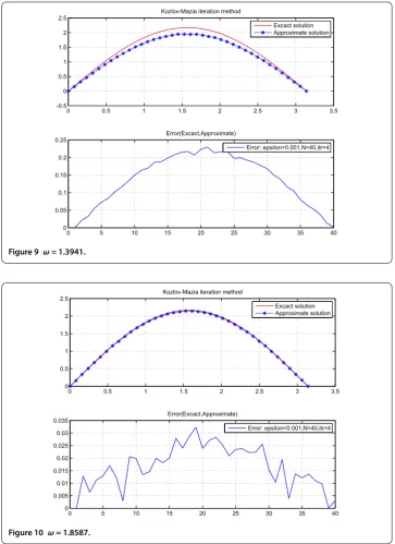
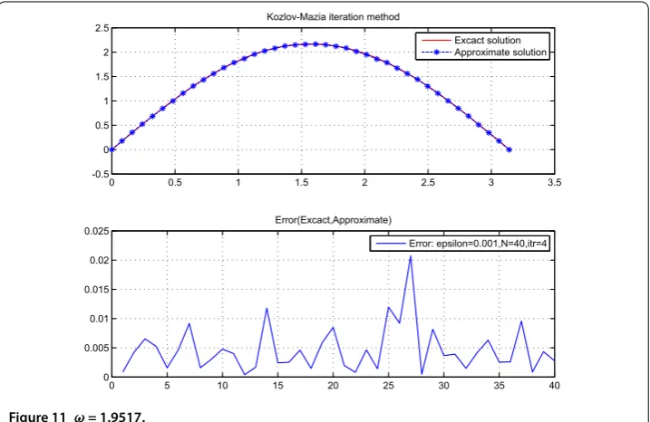
Kozlov-Maz’ya iteration method
By using the central difference with step lengthh= π
N+ to approximate the first derivative uxand the second derivativeuxx, we can get the following semi-discrete problem (ordinary
differential equation):
⎧ ⎪ ⎪ ⎨ ⎪ ⎪ ⎩
uyy(xi,y) –Ah(xi,y) = , xi=ih,i= , . . . ,N,y∈(, +∞),
u(x= ,y) =u(xN+=π,y) = , y∈(, +∞),
u(xi, ) =f(xi), u(xi, +∞) = , xi=ih,i= , . . . ,N,
(.)
whereAhis the discretization matrix stemming from the operatorA= –dxd:
Ah=
hTridiag(–, , –)∈MN(R)
is a symmetric, positive definite matrix. We assume that it is fine enough so that the dis-cretization errors are small compared to the uncertaintyδof the data; this means thatAh is a good approximation of the differential operatorA= –dxd, whose unboundedness is reflected in a large norm ofAh(see [, p.]). The eigenpairs (μk,ek) ofAhare given by
μk=
N+
π
sin
kπ
(N+ )
, ek=
sin
jkπ
N+ N
j=
, k= , . . . ,N.
The discrete iterative approximation of (.) takes the form
fδ
k(xj) = (I–ωKh)kf(xj) +ω k–
i=
(I–ωKh)igδ(xj), j= , . . . ,N, (.)
whereKh=e–
√
Ahandω<
Kh=e
√μ
= ..
Figures -, Table show the comparisons between the exact solution and its computed approximations for different valuesN,Mandε.
Figures -, Table show the comparisons between the exact solution and its computed approximations for different valuesN,k,ωandε.
Conclusion
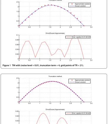
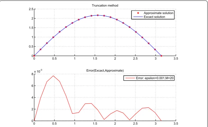
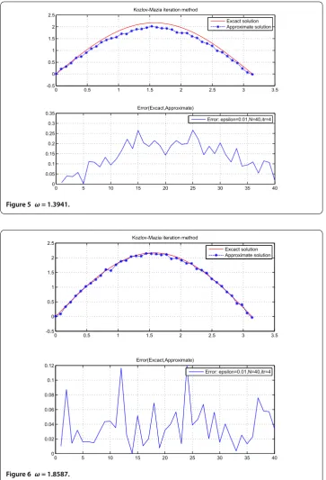
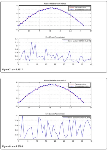
The numerical results (Figures -) are quite satisfactory. Even with the noise levelε= ., the numerical solutions are still in good agreement with the exact solution. In ad-dition, the numerical results (Figures -) are better for (ω= ., ε= .) and (ω= .,ε= .) and the other values are also acceptable.
Figure 1 TM with (noise level = 0.01, truncation term = 4, grid points of TR = 21).
Figure 3 TM with (noise level = 0.001, truncation term = 4, grid points of TR = 21).
Figure 4 TM with (noise level = 0.001, truncation term = 4, grid points of TR = 41).
Table 1 Truncation method: Relative errorEr(f)
N M Er(f)
Figure 5 ω= 1.3941.
Figure 7 ω= 1.9517.
Figure 9 ω= 1.3941.
Figure 11 ω= 1.9517.
Figure 12 ω= 2.2305.
Table 2 Kozlov-Maz’ya method: Relative errorEr(f)
N k ω Er(f)
Future work will involve the error effect arising in computing eigenfunctions and eigen-values of the operatorAon the truncation method. The question is how to obtain some optimal balance between the accuracy of eigensystem and the noise level of input data.
Competing interests
The authors declare that they have no competing interests.
Authors’ contributions
All authors have contributed equally. All authors read and approved the final manuscript.
Author details
1Applied Mathematics Laboratory, University Badji Mokhtar Annaba, P.O. Box 12, Annaba, 23000, Algeria.2Department of
Mathematics, 8 Mai 1945 Guelma University, P.O. Box 401, Guelma, 24000, Algeria.
Acknowledgements
The authors would like to thank the editor and the anonymous referees for their valuable comments and helpful suggestions that improved the quality of our paper. This work is supported by the DGRST of Algeria (PNR Project 2011-code: 8\u23\997).
Received: 13 March 2013 Accepted: 18 July 2013 Published: 2 August 2013 References
1. Cosner, C, Rundell, W: Extension of solutions of second order partial differential equations by the method of quasireversibility. Houst. J. Math.10(3), 357-370 (1984)
2. Levine, HA, Vessella, S: Estimates and regularization for solutions of some ill-posed problems of elliptic and parabolic type. Rend. Circ. Mat. Palermo34, 141-160 (1985)
3. Ivanov, DY: Inverse boundary value problem for an abstract elliptic equation. Differ. Equ.36(4), 579-586 (2000) 4. Dunford, N, Schwartz, J: Linear Operators, Part II. Wiley, New York (1967)
5. Pazy, A: Semigroups of Linear Operators and Application to Partial Differential Equations. Springer, New York (1983) 6. Brezis, H: Functional Analysis, Sobolev Spaces and Partial Differential Equations. Springer, New York (2011) 7. Prilepko, AI, Orlovsky, DG, Vasin, IA: Methods for Solving Inverse Problems in Mathematical Physics. Monographs and
Textbooks in Pure and Applied Mathematics, vol. 222. Marcel Dekker, New York (2000)
8. Shlapunov, A: On iterations of non-negative operators and their applications to elliptic systems. Math. Nachr.218, 165-174 (2000)
9. Krasnosel’skii, MA, Vainikko, GM, Zabreiko, PP, Rutitskii, YB: Approximate Solutions of Operator Equations. Wolters-Noordhoff, Groningen (1972)
10. Krein, SG: Linear Differential Equations in Banach Space. Am. Math. Soc., Providence (1971)
11. Kozlov, VA, Maz’ya, VG: On iterative procedures for solving ill-posed boundary value problems that preserve differential equations. Leningr. Math. J.1, 1207-1228 (1990)
12. Kozlov, VA, Maz’ya, VG, Fomin, AV: An iterative method for solving the Cauchy problem for elliptic equations. U.S.S.R. Comput. Math. Math. Phys.31(1), 45-52 (1991)
13. Bastay, G: Iterative Methods for Ill-Posed Boundary Value Problems. Linköping Studies in Science and Technology, Dissertations No. 392. Linköping University, Linköping (1995)
14. Baumeister, J, Leitao, A: On iterative methods for solving ill-posed problems modeled by partial differential equations. J. Inverse Ill-Posed Probl.9(1), 13-29 (2001)
15. Maxwell, D: Kozlov-Maz’ya iteration as a form of Landweber iteration (2011). arXiv:1107.2194v1 [math.AP] 12 Jul 16. Bakushinsky, AB, Kokurin, MY: Iterative Methods for Approximate Solution of Inverse Problems. Springer, Dordrecht
(2004)
17. Hohage, T: Regularization of exponentially ill-posed problems. Numer. Funct. Anal. Optim.21, 439-464 (2000) 18. Deuflhardy, P, Engl, HW, Scherzer, O: A convergence analysis of iterative methods for the solution of nonlinear
ill-posed problems under affinely invariant conditions. Inverse Probl.14, 1081-1106 (1998)
19. Eldén, L, Simoncini, V: A numerical solution of a Cauchy problem for an elliptic equation by Krylov subspaces. Inverse Probl.25, 065002 (22pp) (2009)
doi:10.1186/1687-2770-2013-178