ASSOCIATION RULE HIDING OVER DATA STREAMS
Ufuk Günay, Taflan
İ
mre Gündem
Computer Engineering Department, Boğaziçi University 34342 Bebek, İstanbul, Turkey
e-mail: [email protected], [email protected]
Abstract. Association rule mining is used in various applications. Also information systems may need to take privacy issues into account when releasing data to outside parties. Due to recent advances, releasing data to other parties may be done in a streaming fashion. In this paper, we introduce a new system in which association rule mining over data streams and association rule hiding for traditional databases are merged. The stream association rule hiding algorithm presented can be applied on both raw data and template guided XML data. The algorithms presented are implemented and tested.
Keywords: Association rule mining, stream mining, association rule hiding.
1. Introduction
Association rule mining techniques [1, 2] have been widely used in various applications such as mar-keting, modern business, medical analysis and website navigation analysis [3-6]. In e-commerce, for instance, a company can understand the behavior of its custo-mers, support decision making and gain an overall significant benefit over its rivals using association rule mining. Thus, some association rule mining algo-rithms have been developed especially for handling transactional data in e-commerce [7-8].
In spite of its benefits in all of these applications, association rule mining can also have a threat to pri-vacy and information security, if not done or used properly [9]. There are a number of realistic scenarios in which privacy and security issues in association rule mining arise. Three challenging e-commerce sce-narios are described in the following.
Scenario 1: First let us consider the scenario of a supermarket and two drink suppliers A and B explai-ned in [10]. Let us suppose that, as purchasing direc-tors of our large supermarket chain, we are negotiating an agreement with Drink Company A. Drink Compa-ny A offers its products at a reduced price, if we agree to give it access to our database of customer pur-chases. We accept the deal and Drink Company A starts mining our customer purchases data. By using an association rule mining tool, Company A finds out that people who purchase products of Biscuit Com-pany X also purchase Drink B. Drink ComCom-pany A now runs a marketing campaign advertising that “you can get 60 cents off Biscuit X with every purchase of a Drink A product”. This campaign cuts heavily into the
sales of Drink B, which in turn may increase the price for us due to decreased sales. During our next nego-tiation with Drink Company A, we find out that with reduced competition, they are unwilling to offer us a low price. Finally, we start to lose business to our competitors, who were able to negotiate a better deal with Drink B. From this aspect, releasing the database is disadvantageous for our supermarket. Therefore, for our supermarket, an effective way to hide sensitive rules while releasing the database is required.
Scenario 2: Let us now consider the following scenario explained in [11]. Suppose that two or more companies have huge dataset records of their cus-tomers’ buying activities. To have an advantage over other competitors, these companies decide to coopera-tively conduct association rule mining on their data-sets for their mutual benefit. However, some of these companies may not want to share some strategic patterns hidden within their own data (sensitive association rules) with the other parties. They would like to transform their data in such a way that these sensitive association rules cannot be discovered.
recommendation. When a client sends its frequent itemsets or association rules to the server, it sanitizes some sensitive itemsets according to some specific policies. The server then gathers statistical information from the sanitized itemsets and recovers from them the actual associations.
In all of these scenarios we ask ourselves the following question. “How can we get rational data mining results that will allow for correct decision making while preventing the disclosure of sensitive information?” In other words, “Is it possible for us to benefit from the collaborations in which we share our data (as explained in Scenarios 1-3) and still preserve some sensitive association rules?” In our proposed system, we try to answer these questions in an environment where real-time data are sent in a streaming fashion.
The rest of this paper is organized as follows. Section 2 explains our proposed system.
Section 3 provides our experimental results. Sec-tion 4 contains the conclusions.
2. Proposed System
2.1. Problem Definition
In this section, we introduce ARDHS, the system that we propose for association rule hiding over streaming data. In ARDHS, we have a single-pass algorithm for hiding all sensitive itemsets in data streams, similar to the landmark windows model explained in [13], when a user-specified minimum support threshold ms Є (0, 1), and a usdefined er-ror threshold ε Є(0, ms) for data pruning phase are given. As explained in [14-15], a data stream can be defined as follows:
Let I = {I1, I2, I3… Im} be a set of literals, called
items. Let the data stream DS = B1, B2, B3 … BN be an
infinite sequence of blocks, where an identifier i is attached to each block, and N is the identifier of the “latest” block, BN. Each block Bi consists of a
timestamp tsi, and a set of transactions; that is, Bi =
[tsi, T1, T2, T3… Tk], where k ≥ 0. Hence, the current
length (CL) of the data stream is defined as CL = |B1|+|B2|+…+|BN|. A transaction T consists of a set of items such that T ⊆I. Moreover, each transaction is given a unique transaction identifier, called TID. A set of items X is also called an itemset and an itemset X
with k items is denoted as (x1, x2, x3… xk), such that X ⊆ I.
The support (defined in [1]) of an itemset X, denoted by sup(X), is the number of transactions seen so far in which that itemset occurs as a subset. An itemset X is called a sensitive itemset if sup(X) ≥
ms*CL. An itemset is called an insensitive itemset if
ms*CL > sup(X).
Hence, given a user-defined minimum support threshold ms Є(0, 1), a user-specified error threshold
ε Є (0, ms) and a data stream DS, our goal is to
develop a single-pass algorithm to hide all sensitive itemsets, in a manner similar to the landmark windows model, of the streaming data using as little main memory space as possible.
2.2. Assumptions
In our proposed system ARDHS, we have the following assumptions:
1) Arriving items in a transaction or an itemset are sorted in lexicographic order.
2) The average size of each block of the data stream is a constant value k, for simplicity (i.e. each block contains k transactions).
3) We hide only rules that are supported by disjoint large itemsets, as done in [16]. If we try to hide overlapping rules, then hiding a rule may have side effects on the other rules to be hidden. This increases the time complexity of our algorithm, since hiding a rule may cause an already hidden rule to haunt back. Therefore we reconsider previously hidden rules and hide them back if they are no longer hidden.
4) We hide one rule at a time. Hiding one rule must be considered as an atomic operation. This is actually related to the third assumption. Since the rules to be hidden are assumed to be disjoint, the items chosen for hiding a rule will also be different for different rules. Therefore, hiding a rule will not have a side effect on the rest of the rules. Thus considering the rules one at a time or all together will not make any difference as explained in [16].
2.3. ARHDS Algorithm
Our algorithm for ARHDS consists of six steps. After describing the steps of the algorithm in detail, we present two examples to illustrate and clarify the system.
Step 1: Reading a block of transactions: In the first step, we read a block of transactions from the data stream.
Step 2: Constructing the Potentially Sensitive Itemset Forest (PSIF) and the Temporary Database (TDb) for the block: To have a fast and an efficient system, the data structures PSIF and TDb are const-ructed and used. PSIF consists of Potentially Sensitive Itemset Trees (PSIT) of item suffixes as explained in [17]. Similarly TDb consists of Temporary Database Trees (TDbT) where the root of each tree represents the first item in a transaction. Both PSIT and TDbT have the same tree structure which is explained in the following.
Each node in the tree consists of four fields:
itemName, support, ChildTrees and parentTree, where
HT is the children item id and the value of HT consists of two fields: the number of occurrences of children items in the tree and the pointers to these occurrences. The construction of TDb can be described as follows. In the current block, let the first transaction to be inserted to the
system be
T1 = (x1, x2, x3, …, xk)which consists of k items. First, ARDHS reads this transaction, T1, from the current block and sets item x1 as the root node for the first tree of TDb. Later x2, x3, …, xk are inserted into the tree one by one, as nodes,
in such a way that the newly inserted one becomes a child of the one inserted just before it (i.e. xi becomes
the parent of xi+1 for i=1, k-1). Consequently, item xk
becomes the leaf node. Each node represents an item of the transaction and a support counter is associated with it. Also a HT will be created for the root node x1 and childrenTree and parentTree HT’s for each of the other nodes. Then ARDHS reads the next transaction
T2 = (y1, y2, y3, …, yk). If y1 is equal to x1 (or if y1 is equal to the item associated with the root node of any tree, ta, in TDb) ARDHS does not add a new tree into TDb but it adds the path of itemset (y2, y3, …, yk) as a
branch (connected to the node associated with x1 with an edge) of the first tree (or ta) of TDb and updates the support of each node accordingly. If the first trans-action, T1, and the next one, T2, have their first r items in common (i.e. x1= y1, x2= y2, …, xr= yr), then the
support of the nodes associated with x1,x2, …, xrare
incremented by one and the path associated with yr+1,
yr+2, …, yk is connected to node xr with an edge
(Please refer to Example 1 for concrete examples and their illustrations). If y1 is not equal to x1 (or if y1 is not equal to the item associated with the root node of any tree in TDb) a new tree which has y1 as the root node and yk as leaf node will be added to TDb.
The construction of PSIF is similar to the const-ruction of TDb but there is a small difference. Before the first transaction T1 is inserted into PSIF, it is converted into the following k small transactions: (x1,
x2, x3, …, xk), (x2, x3, …, xk), …, (xk-1, xk) and (xk). Then
each of these k small transactions are inserted into PSIF as a tree. For each of these small transactions, the tree insertion procedure of PSIF is same as the tree insertion procedure of TDb. After T1 is inserted into PSIF, ARHDS will read the next transaction T2= (y1,
y2, y3, …, yk) and divide it into k small transactions:
(y1, y2, y3, …, yk), (y2, y3, …, yk) , …, (yk-1, yk) ,(yk) and
add these small transactions into PSIF in the same manner.
Each of the remaining transactions in the block is inserted into PSIF and TDbT in the same manner as T2 is inserted.
For XML data, we use the same structure specified above. Additionally, at each leaf node, we store the transaction number for each transaction.
Step 3:Pruning the insensitive itemsets from PSIF. To speed up the execution of ARHDS, we use pruning. The user provided error threshold εЄ(0, ms) is used in pruning the insensitive items from PSIF. Before
starting the hiding process, we repeat Steps 1 to 3 for the remaining blocks of transactions.
Step 4: Finding sensitive disjoint itemsets from PSIF to hide: To hide all sensitive association rules, we developed the following heuristic. Given a minimum support threshold ms Є (0, 1) provided by the user, first we find all sensitive itemsets. Then we sort these sensitive itemsets according to their support. Next, beginning from the sensitive itemset with the highest support, we discover the sensitive disjoint
itemsets to hide. We hide sensitive rules from TDb in Step 5. Then we come back to Step 4 to check if there still exists any sensitive disjoint itemsets. We repeat this strategy until we hide all sensitive association rules from TDb.
Step 5: Hiding sensitive disjoint itemsets and updating TDb: After determining the sensitive disjoint itemsets, we hide them by using a modified version of one of the strategies given in [16]. There are five different algorithms for association rule hiding in [16]. Here, we use the fastest of these algorithms, since we are trying to hide association rules over data streams. Also the algorithm that we use does not introduce new rules. The algorithm is as follows:
To hide sensitive rules, we decrease the support of their generating itemsets until the support is below the minimum support threshold as explained in [18]. If there are more than one large itemsets to hide, we first sort the large itemsets with respect to their size and support. Let Z be the next itemset to be hidden. Let
TSZ be the set of transactions in which Z occurs as a
subset. We hide Z from Database D by removing the items in Z, from the transactions in TSZ, in round robin
fashion. We start with a random order of items in Z
and a random order of transactions in TSZ. Assume
that the order of items in Z is i0, i1, …, in-1 and the order of transactions in TSZis T0, T1, …, Tm-1. At Step 0 of the algorithm, the item i0 is removed from T0. At Step 1, i1 is removed from T1, and in general, at Step k, item is (s= k mod n) is removed from transaction Tk.
The execution stops after the support of the current itemset, to be hidden, goes below the minimum sup-port threshold as explained in [16]. The intuition be-hind the idea of hiding in round robin fashion is fair-ness. Thus no item is over-killed and the chance of having a smaller number of side effects is higher than choosing an item at random and always trying to hide it.
The mentioned algorithm given in [16] hides only selected sensitive itemsets, in ARHDS we hide all sensitive itemsets. When we update the database D, we also update our PSIF structure to go back to Step 4 to check if sensitive itemsets still exist.
Step 6:Sending the updated TDb (the block): After hiding all sensitive items from TDb, the hidden TDb is sent to the receiver.
data. In the second example, we will give only the structure of TDb for XML data, since the other steps are the same.
Example 1: Let us suppose that the data stream consists of two blocks each having five transactions. Let the first block B1 of the data stream be (acdef), (df), (abe), (acdf), (cef), the second block B2 be (bef), (bdg), (def), (bg), (ceg). Let ε = 0.25 be the error threshold for pruning and ms = 0.3 be the minimum support for hiding phases where a, b, c, d, e, f, g are items in the stream.
Step 1: We read the first block B1 from the data stream.
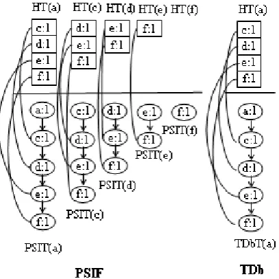
Step 2: 1) First transaction acdef: ARHDS reads the first transaction acdef, inserts item-suffix transactions acdef, cdef, def, ef, f into PSIF and acdef
into TDb. The results are shown in Figure 1. Here, item name and support of each PSIT (Potentially Sensitive Itemset Tree) are presented. Also for each PSIT, HT (Hash Table) for the children nodes are shown. In the following steps, we omit the pointers to the occurrences of each children node for a concise representation.
Figure 1. PSIF and TDb after inserting the first transaction acdef
2) Second transaction df: ARHDS reads the second transaction df, inserts item-suffix transactions df, f into PSIF and df into TDb. The results are shown in Figure 2.
3) Third transaction abe: ARHDS reads the third transaction abe, inserts item-suffix transactions abe, be, e into PSIF and abe into TDb. The results are shown in Figure 3.
4) Fourth transaction acdf: ARHDS reads the fourth transaction acdf, inserts item-suffix transactions
acdf, cdf, df, f into PSIF and acdf into TDb. The re-sults are shown in Figure 4.
5) Fifth transaction cef: ARHDS reads the fifth transaction cef, inserts item-suffix transactions cef, ef,
f into PSIF and cef into TDb. The results are shown in Figure 5.
Figure 2. PSIF and TDb after inserting the second transaction df
Figure 3. PSIF and TDb after inserting the third transaction abe
Figure 5. PSIF and TDb after inserting the fifth transaction cef
Step 3: After processing the first block B1, ARHDS prunes insensitive itemsets from the current PSIF. At this time, ARHDS deletes the PSIT(b) and its corresponding HT(b), and prunes the entry b from all
other PSIT ’s because item b is an insensitive item (i.e.
sup(b) < ε * CL (1< 0.25 * 5)). The resulting PSIF is shown in Figure 6.
Figure 6. PSIF TDb after pruning insensitive item b
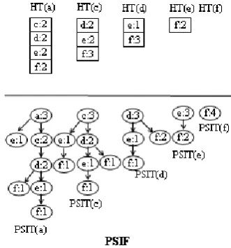
Figure 7. PSIF and TDb after processing the second block B2
After pruning the insensitive items from PSIF, we read the second block B2 for constructing the PSIF and
TDb. The construction process is repeated for block
B2. The resulting PSIF and TDb are given in Figure 7. Next, we go to Step 4 and start hiding sensitive itemsets.
Step 4: After processing the second block B2, first we find all sensitive itemsets with respect to the minimum support threshold ms =0.30 and then we sort these sensitive itemsets according to their support (df with support 4, ef with support 4, ce with support 3, cf with support 3). Next, beginning from the sensitive itemset with the highest support, we compute the sensitive disjoint itemsets to hide (df with support 4, ce with support 3).
Step 5: At this step, we hide sensitive itemsets by using the hiding algorithm we proposed. Pairs of transactions and the items to be hidden are acdef-d, acdf-f, acef-c.
After completing the first iteration we go back to Step 4 to check if there still exists any sensitive itemsets. We find the itemset ef with support 4. Then,
we come back to Step 5 to hide the sensitive itemsets we discovered during the second iteration. Pairs of transactions (to be changed) and the items to be hidden are aef-e, def-f. After the second iteration, we again go back to Step 4 to check if there still exists any sensitive itemsets. Since we find no sensitive itemsets, we continue with Step 6. Figure 8 shows the hidden TDb.
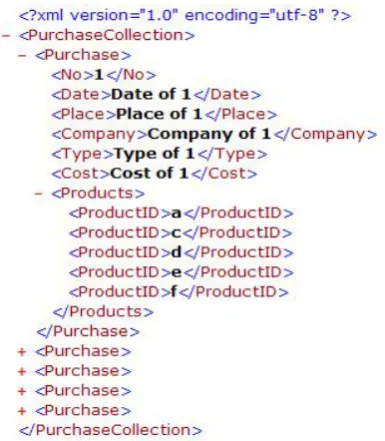
Example 2: Let us suppose that the data stream is the same as that in Example 1, but the stream arrives in XML format. Figure 9 shows the XML stream for block B1.
Figure 9. XML stream for the first block B1
The steps of our algorithm for the template guided XML stream are the same as that for raw data. The only difference is that at each leaf node, we store the transaction number for each transaction. Figure 10 shows the TDb after processing block B1.
Figure 10. TDb for XML data after processing the first block B1
Figure 11 shows the TDb after processing the se-cond block B2 and Figure 12 shows the hidden TDb for the XML stream.
Figure 11. TDb for XML data after processing the first block B2
Figure 12. Hidden TDb for XML data
The reason for storing the transaction number, while hiding an item from a transaction, is as follows. When we send the hidden data to the receiver, we use the transaction numbers to merge the data (on which we apply association rule hiding) with its related part.
3. Experimental Results
output data to the file (sending the hidden database to the receiver).
Later, we analyzed the performance of ARHDS under different parameter settings. We performed tests under different values of parameters such as user-spe-cified minimum support threshold ms Є (0, 1), user-defined error threshold εЄ (0, ms) and block size for the synthetic data. Finally we ran ARHDS for XML data that we generated and compared our algorithm on XML and on raw data for execution time.
The experiments were done on a PC with AMD Athlon (TM) 1.8GHz CPU, 1GB main memory and Microsoft XP Professional. The code for the proposed algorithm is written in Microsoft Visual C# 2.0 and the application development environment Microsoft Visual Studio 2005 is used. We ran our code in VS 2005 environment. We made use of Dictionary (imple-mented as a generic hash table) and List (generic equi-valent of the ArrayList class) classes of the Generic collection in Microsoft Visual C# 2.0.
IBM Synthetic Dataset: To evaluate the perfor-mance of ARHDS, we generated some synthetic data-sets via the IBM’s data generator in [2]. For clarity, we named each dataset in the form of TxxIxxDxx where
T, I and D mean the average transaction length, the average length of maximum pattern, and the total number of transactions, respectively. To evaluate our work, we used four datasets: T7I4D200K, T5I4D10K, T5I4D50K, and T5I4D100K. For T7I4D200K, the number of distinct items is 1000 and for other datasets it is 50. We made use of T7I4D200K for the execution time evaluation of the proposed system. We used other datasets for comparing the hiding time of ARHDS with that of one of the algorithms given in [16].
To evaluate ARHDS on XML data, we generated synthetic XML data by using the synthetic data gene-rated via the IBM’s data generator. We used the syn-thetic data which we generated earlier as the essential part of the synthetic XML data on which we applied association rule hiding.
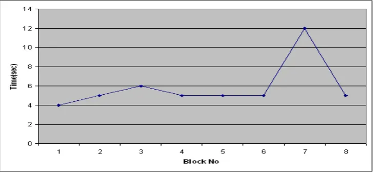
Test 1: The first test is performed to examine the time executed by our algorithm at each step. With ms = 0.0025 and ε = 0.0005, we ran ARHDS on T7I4D200K data. The data are broken into blocks of size 25K for simulating the continuous characteristics of streaming data. Hence there are 8 blocks in this test. Figure 13 shows the execution time for creating PSIF and TDb (prior to association rule hiding).
Figure 13. Execution time for creating PSIF and Tdb
Note that after arrival of each block, we prune PSIF. We expect that the time needed for inserting new transactions into both PSIF and TDb will increase with the incoming new blocks. In Figure 13, we see some points where the execution time decreases. This may be due to the characteristic of the data that we generated. Since there is no sharp increase in execu-tion time we may say that our system creates the data structure for ARHDS reasonably efficiently.
Table 1 shows the number of all sensitive itemsets, the number of disjoint sensitive itemsets chosen after sorting all sensitive itemsets with respect to their sup-port and the number of transactions changed during the hiding process. As expected, all of them decrease from one iteration to the next. Also note that by number of transactions changed we actually mean that the number of different transactions changed as we can change the same transaction several times.
Table 1. Number of all and disjoint sensitive itemsets and the number of transactions changed
Number of all sensitive itemsets
Number of disjoint sensitive itemsets
Number of trans. changed
Iteration 1 20 7 849
Iteration 2 15 5 449
Iteration 3 8 4 192
Iteration 4 5 1 57
Iteration 5 4 1 53
Iteration 6 3 1 40
Iteration 7 2 1 2
In this test, constructing PSIF and TDb takes 47 seconds, hiding disjoint itemsets takes 15 seconds and sending the hidden database to the receiver takes 4 seconds. These results can change with respect to the parameter settings (i.e. hiding time may exceed const-ruction time of PSIF and TDb).
Test 2: To evaluate the scalability of our approach, we performed our second test on user-defined minimum error threshold. We change the minimum error threshold ε while keeping other variables cons-tant (ms = 0.0025, block size=25K, number of blocks = 8). Figure 14 shows execution times for different minimum error threshold. As there is no sharp in-crease or dein-crease in the graph, we may say that our approach is stable.
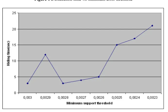
Test 3: As the third test, to examine the execution time of hiding the association rules for the disjoint sensitive itemsets, we ran ARHDS with different mini-mum support threshold ms while keeping other variables constant (ε = 0.0005, block size=25K, num-ber of blocks = 8). Figure 15 shows the execution time for hiding disjoint sensitive itemsets changing with different minimum support threshold values. Note that in addition to the time required for the hiding process, execution time includes the time spent for finding all sensitive itemsets and getting the disjoint sensitive itemsets. Figure 15 shows that our heuristic for hiding all sensitive itemsets from the database gives reason-ably efficient results.
Figure 14. Execution time vs. minimum error threshold
Figure 15. Execution time for hiding vs. minimum support threshold
Table 2 shows the hiding time and the number of transactions changed for different minimum support threshold values. We see that if the minimum support threshold value decreases, the number of transactions changed increases but hiding time does not always
Table 2. Execution time of ARDHS at each step
ms execution time Number of transactions changed
0,0030 3 620
0,0029 12 740
0,0028 3 899
0,0027 4 1098
0,0026 5 1344
0,0025 15 1642
0,0024 17 1968
0,0023 21 2487
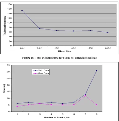
Test 4: The fourth test is performed to examine the time taken by our ARHDS for different block size while keeping other variables constant (ms = 0.0025 andε = 0.0005). Figure 16 shows the total execution time of ARHDS with changing block size for T7I4D200K data. Having the highest execution time
with block size 10K may be due to the highest number of pruning or the characteristics of the data tested. Figure 16 shows that the system is stable under dif-ferent block sizes.
Raw data XML data comparison: The fifth test is performed to compare the execution time of our algorithm for raw data and that for XML data that we generated. For comparison, we used the same para-meters (ms = 0.0025, ε = 0.0005, and the block size = 25K) in both executions. Also T7I4D200K is used for generating raw data and XML data. Figure 17 shows the execution time to create PSIF and TDb for raw data and XML data (prior to association rule hiding). From Figure 17, we see that the execution time grows sharply at the last block. This is due to the fact that we store parts of XML data that we do not use for association rule hiding but for sending back to the receiver. File sizes for raw data and XML data are 6MB and 120MB, respectively.
Figure 16. Total execution time for hiding vs. different block size
Figure 17. Comparison of execution times to create PSIF and Tdb
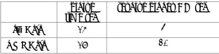
Table 3 shows the hiding time and time of sending the hidden database (DB) to the receiver for raw data and the XML data. As expected, there is not much
Table 3. Hiding time and time of sending hidden DB to receiver
hiding time(sec)
sending hidden DB (sec)
Raw Data 15 4
XML Data 17 20
Comparison with another hiding Algorithm: As explained in Section 3, we modified and adopted one of the algorithms given in [16] for the sensitive rule hiding part of ARHDS. We also compared the hiding time of our algorithm with that of the mentioned algo-rithm in [16].
The algorithm in [16] hides 5 or 10 chosen rules but in ARHDS all sensitive rules above a user spe-cified minimum support threshold are hidden. From this view point, a correct comparison of our algorithm with that in [16] is not possible. Yet we ran ARHDS with different minimum support thresholds and with different size databases, similar to those given in [16] to get some idea about the hiding time of our system. The results show that the two algorithms have similar hiding times.
4. Discussion and conclusion
Mining data streams is an interesting and challen-ging research field. Also, due to the fact that recent advances in data mining algorithms have increased the disclosure risks that one may encounter when relea-sing data to outside parties, association rule hiding is another interesting and challenging research field [16]. We merged these two challenging research areas. In this paper we introduce a novel system we named ARHDS for discovering and hiding association rules over data streams.
ARDHDS mainly consists of two parts. The first part creates our data structure to discover sensitive itemsets to hide and the second part hides these item-sets from the data we stored. For the first part we use a prefix tree structure similar to that in [17]. In the second part we hide sensitive itemsets by decreasing their supports.
We ran ARHDS with different parameter settings to examine the scalability and stability of our algorithm. We also tested our proposed system on both raw data and the XML data. We have found that our algorithm is reasonably fast and efficient.
Our approach is open for improvements. It remains a future work to make a more efficient implementation for our proposed system.
References
[1] R. Agrawal, T. Iimielinski, A. Swami. Mining Asso-ciation Rules Between Sets of Items in Large Databa-ses. Proc. of the 1993 ACM SIGMOD International Conference on Management of Data, 1993, 207-216. [2] R. Agrawal, R. Strikant. Fast algorithms for mining
association rules. Proc. of International Conference on Very Large Data Bases, VLDB, 1994, 487-499.
[3] S. Halatchev, L. Gruenwald. Estimating Missing Values in Related Sensor Data Streams. Proceedings of the 11th International Conference on Management of Data (COMAD 2005),2005, 83-94.
[4] D. Erik, A. Lopez-Ortiz, J. Munro. Estimation of In-ternet Packet Streams with Limited Space. Procee-dings of 10th European Symposium on Algorithms, 2002, 348-360.
[5] D. Cai, G. Pape, J. Han, M. Welge, L. Auvil. MAIDS: Mining Alarming Incidents from Data Streams. Proceedings of the 2004 ACM SIGMOD International Conference on Management of Data,
2004, 919-920.
[6] H. Kargupta, R. Bhargava, K. Liu, M. Powers, P. Blair, S. Bushra, J. Dull, K. Sarkar, M. Klein, M. Vasa, D. Handy. VEDAS: A Mobile and Distributed Data Stream Mining System for Real-Time Vehicle Monitoring. Proceedings of SIAM International Con-ference on Data Mining, 2004, 300-311.
[7] A. Geyer-Sshulz, M. Hashler. Comparing Two Re-commender Algorithms with the Help of Recommen-dations by Peers. In: WEBKDD 2002 – MiningWeb Data for Discovering Usage Patterns and Profiles, LNCS, Springer,2003, 137-158.
[8] J.A. Major, J.J. Mangano. Selecting among rules in-duced from a hurricane database. Journal of Intelligent Information systems,Vol.4, No.1, 1995,39-52. [9] V.S. Verykios, E. Bertino, I.N. Fovino, L.P.
Pro-venza, Y. Saygin and Y. Theodoridis. State-of-the-Art in Privacy Preserving Data Mining. ACM SIGMOD Record, Vol.3, No.1, 2004, 50-57.
[10] Y.H. Wu, C.M. Chiang, A.L.C. Chen. Hiding Sen-sitive Association Rules with Limited Side Effects.
IEEE Trans. Knowledge Data Engineering, Vol.19,
No.1, 2007, 29-42.
[11] S.R.M. Oliviera, O.R. Zaiane. Protecting Sensitive Knowledge by Data Sanitization. Proceedings of Third IEEE International Conerence on Data Mining, 2003, 613-616.
[12] S.R.M. Oliviera, O.R. Zaiane, Y. Saygin. Secure Association Rule Sharing. Proceedings of the 8th Pacific-Asia Conference on Advances in Knowledge Discovery and Data Mining, LNCS, Springer, 2004, 74-85.
[13] Y. Zhu, D. Shasha. StatStream: Statistical Monitoring of Thousands of Data Streams in Real Time. Procee-dings of International Conference on Very Large Database, VLDB, 2002, 358-369.
[14] S. Guha, N. Koudas, K. Shi. Data Streams and Histo-grams. Proceedings ofACM Symposium on Theory of Computing, 2001, 471-475.
[15] N. Jiang, L. Gruenwald. Research Issues in Data Stream Association Rule Mining. ACM SIGMOD Record, Vol.35, No.1, 2006.
[16] V.S. Verykios, A. Elmagarmid, E. Bertino, Y. Saygin, E. Dasseni. Association Rule Hiding. IEEE Transactions on Knowledge and Data Engineering, Vol.16, No.4, 2004, 434-447.
[17] H.F. Li, S. Lee, M. Shan. An Efficient Algorithm for Mining Frequent Itemsets over the Entire History of Data Streams. International Workshop on Knowledge Discovery in Data Streams, 2004.
[18] A. Elmagarmid, M. Atallah, E. Bertino, M. Ibra-him, V.S. Verykios. Disclosure Limitation of Sen-sitive Rules. Proceedings of Knowledge and Data Exchange Workshop, 1999, 45-52.