Pipe defect assessment made by strain-based design

Pipe defect assessment made by

strain-based design

by G. Pluvinage

FM.C, Silly sur Nied, France

A B S T R A C T

S

TRAIN-BASED DESIGN (SBD) is preferred for situations where the loading of a pipeline is due to forces other than the internal pressure and produce large stress and strain in the pipe wall.

Under constraint conditions due to the presence of defect, tensile strains are increased due to stress concentration and the critical strain is reduced due to stress triaxiality. Such cases can be considered in design using Defect Assessment Procedures (DAP).

This paper presents an extensive review of SBD methods used for pipe defect assessment as:

1. critical global strain as a criterion for pipe defect assessment; 2. critical local strain as a criterion for pipe defect assessment; 3. strain intensity factor as a criterion for pipe defect assessment; 4. notch ductility factor (NDF);

5. strain-based design based on J integral; 6. strain-based design based on CTOD.

This presentation follows a rapid description of the mechanism of ductile failure, the influence of triaxiality, and loading mode through Lode angle.

Key words: ductile failure, strain-based design, pipe defect assessment

1. Introduction

Traditional pipeline design methods are stress-based, where the applied stress must remain below the standard minimum yield strength (SMYS). SMYS is generally defined as the stress measured at 0.5% total strain on the stress strain curve. Stress-based design limits the longitudinal strain to less than 0.5%. Stress based design criteria do not provide a good indication of the margin to failure because it ignores the strain hardening capacity of the material. Implantation of pipe lines in harsh environment as artic or deep ocean conditions, induces challenging conditions for design especially in the cases where displacement-controlled loads are the predominant design condition. In this case, strain-based design (SDB) is applied instead of stress-based design to build safer pipelines and to assure the integrity of the lines along their lifetimes. It requires steels to have a large strain hardening capacity, long uniform elongation, and good toughness to achieve a well-defined and sufficient plastic deformation.

ARTICLE INFO

Received: 7 March, 2018 Revised: 14 September, 2018 Accepted: 8 October, 2018

Strain-based design (SBD) is preferred for situations where the loadings of the pipelines are due to forces other than the internal pressure and produce large stress and strain in the pipe wall. Such loadings can be generated by either permanent or transient ground deformation caused by seismic activity, soil subsidence, slope instability, frost heave, thermal expansion and contraction, landslides, pipe reeling, pipe laying, and other types of environmental loading. Therefore SBD is appropriate where the stresses and strains exceed the proportional limit and where the peak design loads will be reduced when the material strains. When strain and stress are not proportional, stress-based methods become very sensitive to details of the material stress strain behaviour and to any safety factors. Strain-based design avoids these problems.

The methodology of SBD is developed in connection with the limit states. There are several limit states associated with SBD : tensile rupture (material limit state) and compressive buckling (material and serviceability limit states).

The fundamental equation for SBD relates the comparison of the applied strain or strain demand e_d with the permissible strain or strain capacity e_c

ε_d ≤�ε_{c (1)}

A maximum strain limit of 10% (0.1) is generally applied in the absence of additional engineering information. A safety factor f_s is applied on limit strain e_l when information is

provided and the strain capacity is defined as:

ε_c εl s f

=� ₍₂₎

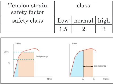
Table 1 gives the safety factors according to the safety classes for tension. They are different for compression buckling.

Figure1 gives a diagram of the difference between stress-based design and SBD. Several codes described strain-based design of pipelines. These codes can be placed in three general categories: those that provide a comprehensive overall pipeline standard that includes requirements both for stress- and strain-based design (DNV 2000 [1], CSA Z662 [2]), those that specifically allow strain-based design but do not provide extensive provisions related to strain-based design (B31.8 [3], API 1104 [4] ), and those that provide information on strain-based design related to a specific subgroup of pipelines (API RP 1111 [5]).

Under constraint conditions due to the presence of defect, tensile strains are increased due to stress concentration and the critical strain is reduced due to stress triaxiality. Such cases can be considered in design using Defect Assessment Procedures (DAP). SBD is now introduced in DAP as recommended method in some code [6]. These methods can be placed in for categories:

• global strain methods based on plastic instability;

• local strain method based on local strain criteria taking into account stress triaxiality and loading mode;

• description of the strain distribution at defect tip by a strain intensity factor, a notch stress intensity factor or a notch ductility factor;

• relation between crack driving force and global strain, the crack driving force is expressed in terms of CTOD or J integral.

The above-mentioned methods are described in the following sections.

2. Failure strain for ductile failure by void nucleation

If D₀ is the diameter of the net section of the specimen and Df the final diameter of the same section, the critical strain is defined as:

ε_f

f

Ln D

D

= 

  



  

2 0

(3)

This phenomenon can be explained by the fact that the modification of the stress radius modifies the stress triaxiality b, defined as the ratio of the hydrostatic stress s_m and the

equivalent stress s_eq.

β σ

σ =�m

eq

(4)

In the case of a notched specimen as

represented in Fig.1, the stress triaxiality is given by the Bridgman formula:

β

ρ

= +  +

  



  

1

3 1 4

0

ln D ₍₅₎

It can be seen like on Fig.3 that the critical strain e_f decreases exponentially with the stress

triaxiality according to:

ε_f =�ε_n�+Aexp

(

−Bβ

)

(6)

where e_{n is the nucleation strain and A and B material constant. Several authors [7, 8, 9, 10,}

11] have notice that the parameter B has a value close to 1.5.

The critical strain is also influenced by the strain rate and decreases when the strain rate increases but the nucleation strain is few affected by the strain rate. Influence of triaxiality and strain rate can be expressed by the following relationship:

ε α

β

f=n +_{1/n m+} (7)

where a is a material constant, n the strain hardening exponent and m is the strain rate sensitivity parameter Fig.4.

3. Ductile fracture by voids nucleation and growth

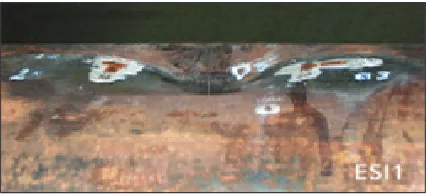
The ductile fracture aspect consists of cup and cones as can be seen in Fig.5.

This aspect results from a mechanism involving void nucleation, growth and ligament instabilities as can be seen on Fig.6.

Void nucleation occurs according to a local stress or energetic criteria. Void growth is sensitive to stress triaxiality and strain amplitude. Figure 7 indicates that the relative void growth is

Tension strain

safety factor class

safety class Low normal high

1.5 2 3

Table 1. Safety factors according to the safety classes for tension

Fig1. Diagram of the principle of stress-based design and strain-based design (SDB)(SMYS standard minimum yield strength, sd stress demand, ed strain demand, and el

proportional to stress triaxiality and strain amplitude as mentioned by several authors [12, 13]:

r

r L M

c

f

0

= +_ . .β ε_{ (8)}

in which r₀ is the initial radius of the particle and r_c its value at failure.

Void growth rate dr is sensitive to stress triaxiality as described by numerous model such as Rice and Tracey [12]. In this model spherical void of radius r without interactions with other particle increase its size by an increment which depends on stress triaxiality:

dr=Ar d. ._{0 eq pl,} . .

( )

1 5β (9)

where A is a constant and r₀ the initial radius of the particle. Assuming no incompressibility:

ε_{f Ln} rc r

=



  



  

0

(10)

in which r_c is the size of the voids at failure. Rice and Tracey’s [12] law can be written as:

ε_{f pl,} =B exp.

(

−1 5. β

)

(11)

Another form of Rice and Tracey’s law can be written as:

ε_f =ε_n +

(

ε_{f smooth,} −ε_n

)

exp

(

−0 5 1 5. − . β

)

(12)

where e_f,smoothis the failure strain for a smooth specimen. Other criteria are based on damage as Lemaitre’s criterion [14].

ε_f = ε + +ε −ε

   

   

+    

   

n s

n nf smooth

s n

n

2 1

2 ₁ 2

,

ss n

vs

s n

R

+    

   

+ 



      



     

1 1/2 1

  

   

(13) Fig.2. Evolution of the critical strain in steel XC18 with

where s is the exponent of the power damage law and R_v some kind of triaxiality parameter.

Bonora’s criterion [15] is given by:

ε ε ε

ε

f n

f smooth n

R_v

= 

  



  

. ,

/ 1

(14)

A comparison of the following model Rice and Tracey (RT) Lemaitre (Lem) and Bonora (Bon) is given in Fig.8 and obtained on 2024 aluminium alloy.

4.Critical strain for shear and ductile fracture

Experimental results (Fig.9) indicate that shear ductile fracture does not follow an exponential decrease with triaxiality but is sensitive to loading mode [16,17].

Critical strain e_f can be described by the following equation for shear fracture:

ε

β f

C =

+

1

(15)

and for ductile failure by void growth:

ε β f

D

=

(16)

in which C and D are material constants.

The azimuthal dependence of the fracture strain envelope is described by six peaks (at generalized tension and compression conditions) and six valleys (at generalized shear conditions). In other words, ductile fracture of solids is more sensitive to shear type of loading. This consideration is based on the observation of many experiments.

4.1 Description of the effect of stress triaxiality and loading mode by Wierzbicki and Xue model In order to have a general description of the influence of the stress triaxiality and loading mode, Wierzbicki and Xue [18] have proposed a model where the loading mode is described by the Lode angle.

The Lode angle can be considered, rather loosely, a measure of loading type. The Lode angle varies with respect to the middle eigenvalue of the stress. The Lode angle is connected to the third invariant of the stress tensor:

J₃ det s 1tr s s s s s s_{ij jk ki}

3

1 3

=

( )

=

( )

. . = (17)

Fig.4. Evolution of the growth strain ef - en in steel XC18

with parameter b(1⁄(n+m)) _[10].

Fig.6. Diagram of the ductile failure mechanism.

Fig.7. Influence of stress triaxiality on the parameter r_c/r₀.ef.

Fig.8. Comparison of Rice and Tracey (RT) Lemaitre (Lem) and Bonora (Bon) models; data obtained on 2024 aluminium alloy.

Fig.9. Influence of stress triaxiality on ductile failure by voids growth or by shear.

There are many definitions of Lode angle that each utilize different trigonometric functions: the positive sine, negative sine, and positive cosine (here denoted q_s, _q

s, and qc, respectively) see Table 2.

sin sin cos J

J

s s c

3 3 3

3 3

3 2

3 2

θ θ θ

( )

=−

( )

=

( )

=    



  

.

/

(18)

with: θ_s =π−θ_c

6

(19)

Generally another definition of the Lode angle is used:

θ πθ

θ

π π

L s c arccos

J J

= = − = − 

   



   



.

/

6

1 6 1 2 3 3

2

2 23 2

  



   

(20)

This definition allows a graphical representation of the stress state between

[−π/6 < θ π< /6].

One notes the existence of the Lode parameter L:

L II III

I III

≅− = −

− −



  



  

.

θ σ σ

σ σ

2 1

(21)

4.2 Wierzbicki and Xue model [18]

In the Wierzbicki and Xue model, the failure strain is sensitive to hydrostatic pressure s_m

and the Lode Angle q_L. Each parameter affects independently the failure strain and is governs by a specific function according to:

ε σ θ_{f m L f} µ_σ σ_m µ_θ θ_L

m L

, _, * *

(

)

= ₀

( )

( )

(22)

µ σ σ σ

σ σ

σ_m m m

m

m m l

qlog

l

exp q

( )

= −  −   



  

≥ − 

 

1 1

1 1

,

.

,

   

  

   

( )

=

< − 

  _ 

   if

if

exp q

m m

m m l

µ σ

σ σ

σ 0

1 1

.

,

   

(23)

s_m,l is the hydrostatic limit pressure as indicated in Fig.10, and q a material parameter. The dependence with the Lode angle is given by:

µ θ γ γ θ

π

θ_L L

L k

( )

= + −

(

)



   



  

1 . 6 ₍₂₄₎

In order to get a presentation with six petals, the m_{qL(qL) is presented in polar coordinates.}

µ θ

θ θ

θ_L L

L r

( )

=

−

(

0 0

)

cos (25)

r₀

2

2 3 1

=

− +

γ

γ γ (26)

θ γ

γ γ

0 1 ₂

2 3 1

=

− +

−

cos (27)

Fig.10. Azimuthal dependence of the fracture strain

Fig.12. Polar dependence of the Lode angle dependence function.

Fig.13. Critical gross strain versus defect ratio for tensile failure in presence of defect and associated with plastic instability according to Denys (2007).

Fig 14. Critical buckling strain for pipe in bending, Denys [19].

g is a material parameter. By increasing the values of g one increases the deep of the valleys of the failure strain envelope in shear conditions as indicated in Fig.12.

5.Critical global strain as a criterion for pipe defect assessment

Strain-based design generally refers to pipeline designs expected to have longitudinal strains greater than 0.5%. Strain-based design encompasses both applied strain demand and strain resistance. At least two limit states are associated with strain-based design: tensile failure and compressive buckling. Strain-based design in recent years has been driven primarily by the need to construct pipelines in the arctic regions, deep-water offshore and other areas with high probability of large ground movements. Cases of in service plastic strain were also observed through the history of pipeline usage due to soil movement on unstable slopes, mining subsidence, and seismic loadings. Confidence developed from the resistance of steel pipelines to these loadings and the understanding of pipe behaviour compared to known strains in installation and test has allowed pipeline designers to include strain-based design for in-service plastic strain.

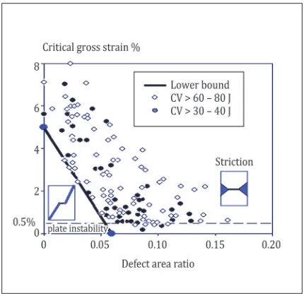
Tensile failure in the presence of defect is caused by plastic instability. Two kinds of instabilities can be developed:

• for defect less than a critical value, plastic instability with plastic band at 55° of the direction of loading (plate instabilities) are associated with large plastic strain.

• for defect larger than a critical value, instability by striction associated with small plastic strain is developed.

The transition of these two types of instabilities described in Fig.13 has been exploited to develop a critical defect size failure criterion initially associated with a 1% critical gross strain but now with a reduced 0.5% strain.

methods for assessing tensile failure resistance of pipelines by engineering critical assessment become fewer when the plastic strain exceeds 0.005 (0.5%) and fewer still as the strain increases to 0.02 (2%) or more. These engineering critical assessment methods are used to demonstrate the sizes and types of imperfections that can remain in pipes and welds for high-strain service. In compression, the failure modes relate to several varieties of buckling. The entire length of pipeline segment can buckle like an Euler beam, either vertically or horizontally. Alternatively, or in combination with these modes, a pipeline may buckle a local area of the pipe wall. Internal pressure increases resistance to local buckling because the tensile hoop stress creates helps for the pipe to resist the diametrical changes that occur locally at buckling. External pressure reduces the resistance to local buckling. It can also create the possibility of a propagating buckle, a local buckle that extends along the pipe leaving a section of collapsed pipe.

Yield strength should be recognized as an important parameter for assessment of the risk of local buckling, particularly for materials with a strong change of slope in the stress-strain curve near the yield point. Higher yield strength correlates to a lower critical strain for local buckling Fig.14.

Several codes have provisions that apply to strain-based design of pipelines. The first limited residual longitudinal strain to below 0.002 0.2%) for areas that are not reeled or pulled through a J-tube or have similar displacement-loading conditions imposed. This limit was for global strain as local strain was limited to 0.02 (2%) at areas of variable stiffness. Permanent curvature methods, such as reeling or J-tube installation could have 0.02 (2%) bending strain or 1% with bending and straightening. The safety factor used for the engineering critical assessment of the Northstar pipeline can be used as an example for those cases where very high safety levels are required for strain-based design. There a safety factor of 3 on strain was applied, somewhat higher than the safety factor on buckling from the compression side of the pipe in bending. The use of the “strain based” design criterion in offshore pipeline technology has widely increased in the last years since a general consensus has been developed about the fact that, in many circumstances, it is more valid than a “stress based” design criterion.

6.Critical local strain as a criterion for pipe defect assessment

6.1 Description of the stress distribution in a log-log chart

The distribution of the local opening strain distribution in log-log graph exhibits 3 particular zones as one can see in Fig.15. This local elastic strain distribution is relative to a single notch tensile specimen.

Table 2. Variation of the different Lode angle with stress state Stress state

σ₁ ≥σ₂ ≥σ₃

Range

Triaxial compression (TXC)

Shear (SHR)

0 0

Triaxial extension

(TXE) 0

q_{* q*} q_c

− ≤π θ ≤π

6 * 6

σ₁ ≥σ₂ =σ₃ p

6

− ≤π θ ≤π

6 * 6 0

3

≤θ_c ≤π

−π

6

p

6

p

3

p

6

−π

6

σ₁ =σ₂ ≥σ₃

Fig.15. The distribution of the local opening strain distribution in log-log graph (K.T specimen: notch depth a = 15mm; notch radius r = 1mm).

Fig.16. Evolution of a parameter with the notch radius and the non-dimensional notch depth (a notch depth, W specimen width).

Fig 17. Evolution of critical effective strain versus non-dimensional notch depth.

Fig.18. General aspect of a plain dent in a pipe.

• Zone I the maximum strain is related to the stress concentration factor

k_{t max}ε = k_{t g}ε (28)

• Zone II Between zone I and zone III • Zone III where the opening strain s_yy distribution versus distance r is governed by a power law

ε

π

ρ α

yy K

r =

( )

,

2

(29)

a is the slope of the local opening strain distribution in log-log graph K_{r, e} the notch strain intensity factor.

• Zone IV where the opening strain decreases rapidly.

The boundary between the zones II and II is situated at distance X_ef the effective distance. At this distance corresponds the effective deformation e_ef. For the local strain distribution in zone III, the producte e_ef .(X_ef)a is constant and equal to the notch strain intensity factor K_r,e. At critical load corresponds the

critical effective deformation e_ef,c, the critical effective distance X_ef,c and the critical notch strain intensity factor K_r.e,c.

ε_{ef c,} . 2

(

πX_{ef c,}

)

α =K_{ρ. ,c} (30)

The local strain distribution exhibits a maximum e_max which decreases exponentially with the notch radius notch (Stress concentration effect). The effective distance increases with notch radius and decreases linearly with depth for small values of a and then parabolic for large values. The a parameter decreases with notch radius as can be seen in Fig.16.

The critical effective strain varies with the notch depth and the notch radius (Fig.17).

6.2 Application to dents assessment

Fig.19. Definition dent depth H.

Fig.20. Stress distribution ahead of defect tip (gouge and gouge plus dent) [29].

Fig.21. Evolution of critical stress with temperature (I - brittle fracture domain, II_A and II_B- elasto-plastic, III - ductile) [31].

Fig.22. Simplified (a - left) and real (b - right) strain distribution at defect tip.

change in curvature of the pipe wall without reduction of pipe thickness. The dent depth (H) is defined as a distance between undamaged cross section and damaged cross section (see Fig.19). In other words, plain dents are defined as dents having no injurious defects such as a gouge and possessing a smooth profile (they are often classified as smooth dents).

The critical variables relating to plain dents are:

• dent depth;

• pipe geometry (ratio of diameter to wall thickness);

• curvature profile of the dent; • service pressure;

• applied cyclic pressure range.

The depth is the most significant factor affecting the burst strength and the fatigue life of a plain dent. In literature, we have found some acceptability limits of dent depth. Assessment is made generally by empirical rules: if the dent depth is more than one tenth of the pipe diameter, repairing is then mandatory. It has been seen than plain smooth dent depths up to 8% of pipe diameter [21] and possibility 24% [22] do not significantly reduce the burst strength of a pipeline.

The API 579 code [23] treats plain dents. Dents are dangerous if they occur on longitudinal weld seams because then cracks can develop. Several sources report that dented weld seams can have very low burst pressures [24].

A later study was carried out by the European Pipeline Research Group (EPRG) [25], which discovered that for plain smooth dents located away from pipe weld seams, dent depths up to 10% of the pipe outside diameter will not fail at membrane stress levels below 72% of the SMYS:

H

D_e £10%

(31)

The measured depth on the operational pipeline must be corrected before this criterion can be applied. EPRG found the correlation between the dent depth on a non-pressurized pipe and a pressurized pipe to be as follows [24, 25]:

H =1 43. H₀ (32)

where H₀ is the depth of the dent in the pressurized condition in (mm). Therefore, the EPRG limit for plain dents in a pressurized pipe is [24, 25]:

H₀/D_e< 7% (33)

Orynyak et al. [26] had proposed that the dent region fails by plastic hinges mechanisms. The ultimate plastic bending moment is then reduced by a factor which depends on dent geometry.

The assessment of a dent can be made using a local strain criterion assuming that the local maximum critical stress e_l,c reaches the failure strain e_f:

ε_{l c,} =ε_f (34)

Finite element computing gives the stress distribution ahead of the gouge tip. Using the procedure described previously, the effective stress was obtained and used as a failure criterion. An example of stress distribution at gouge tip can be seen in Fig.20 for the gouge alone and for the gouge and dent defect. One notes that the stress distribution is similar with an important change in slope in zone III of the stress distribution. The similarity between the stress distributions supports the assumption that the combined defect gouge + dent can be treated by the same solution as that of a simple gouge i.e. the Volumetric Method. The high change of the slope in region III is due to the bending moment induced by the movement of dent walls under internal pressure.

One notes that the effective stress decreases with dent depth. The additional bending stress distribution modifies the final distribution and reduces its severity and consequently the stress triaxiality b.

β σ

σ =� m�

eq (35)

where s_m is the hydrostatic stress, and s_eq is the Von Mises equivalent stress. Due to the fact that the failure of the pipe is ductile and taking into account the fact that ductile failure is sensitive to stress triaxiality, the average value of the stress triaxiality was computed for the burst pressure:

β_c β

X ef

r dr c X_ef

= 1

∫

0 ( ) (36)

Here dent assessment is based ased on simple local strain criterion and considers also the dent as an indentation. Based on various assumptions, many criteria for ductile fracture due to deep drawing have been proposed. Here we use the criterion proposed by Oyane et al. [28]:

I

C C d

f

= 1

∫

+ =1

2 0 1

( )

ε

where e_f is the failure strains, s_m is the hydrostatic stress, b the stress triaxiality and C₁ and C₂ are the material constants. To determine the material constants C₁ and C₂ in Equn 33, tests have to be performed under two types of stress conditions: uniaxial and plane-strain tension tests. By finite element simulation, I integral is calculated for each element and each deformation step. From Equn 33, it can be assumed that the fracture criterion is satisfied in a given element, provided that I integral reaches the value of one, so fracture occurs [27].

7. Strain intensity factor as a criterion for pipe defect assessment

For elastic plastic or ductile fracture, the Russian method M - 02 - 91 [30] recommends to use a strain fracture criterion based on the strain intensity factor KIe. The strain intensity factor is similar to the stress intensity factor used to describe the stress distribution at a crack tip in linear elasticity. It decreases the strain distribution at crack tip in elasto-plastic situation. The fracture criterion is written:

K_Iε =K_{I cε,} (38)

where K_Ie,c is the fracture resistance or critical strain intensity factor. Determination of the critical strain intensity factor is not standardised in the Russian code M - 02 – 91 and is generally obtained from the stress intensity factor K_I:

K K I if

K K I I

I I y

p

g y

I I y

p

g y

n

ε

ε

σ σ σ

σ σ σ

=

(

)

≤

=

(

) (

)

( )−

/ .

/ . . / . 1 /nn n( )+1 ifσ_g >σ_y (39)

I is a parameter to take into account the biaxiality of loading; n is the strain hardening exponent; p is a parameter characteristic of the material; s_y the yield stress and s_g the applied gross stress. In the code M - 02 – 91, fracture resistance K_Ie,c evolution with temperature is differently defined in the elastic plastic and ductile domains. The domain limits are defined in Fig.21. s_{c is the critical global stress; I brittle fracture domain; IIA and IIB are the elasto-plastic}

domains σ_c T σ σ

g y

R and

≤ _{0 2,} > respectively; III ductile failure domain. For point 1, the critical gross stress is equal to σ_g =K_{F y}σ , at point 2 s_g = , and at point 3 σ_g =K_{F ul}σ , K_F is defined by Equn 36 and s_ul is the ultimate stress.

K_F is a geometrical parameter which characterise a surface semi-elliptical crack of depth a,length 2c in a plate of thickness t.

K a t

a t a t

F =

+

(

) (

)

 

/ / / /

1 2 π (40)

The limit temperature of domain II_A and II_Bis determined by the relationship:

T T ln K

ln

b t

F

y T

ul T

= +

( )

(

)

/

,2 70

σ σ (41)

The first transition temperature T_t,1 determines the limit of domain II_B. It is connected to the second transition temperature T_t,2 by the following relationship:

The critical strain-intensity factor in the elasto-plastic domain T_t,2 < T ≤ T_b according to method is given by:

K_{I c} K_Ic T_ul T_y T_ul T_ult

, = *.

(

/

)

. / ,

 

 _

σ σ α σ σ 2 (43)

where K_Ic* is given by

K_Ic* ₌K Y_{F. .σ}T_yt,2_. a_/1000 (44)

where Y the geometry correction factor is given by:

Y a c

a c a t

= −

(

)

−

(

−

)

( )

        . / . . / . / . .

2 0 82

1 0 89 0 57 3 1 5

3 25

(45)

s_yTt _{is the yield stress at temperature T. Exponent a = (T-T}

t,2)⁄70 varies linearly with temperature. In the elasto-plastic domain II_BT_b < T ≤ T_t,1 the critical strain intensity factor is:

K K

K

I c Ic

F ul T y T y T y T_t , * / . . / . / ,

= 1

(

_{σ σ}

)

β ϑ _{σ σ} 2_

(46)

b is a parameter and is temperature dependant.

β σ σ σ σ = − +

( )

(

)

−

( )

(

)

     

T T ln K

ln ln K ln t F y T ul T F y T ul T , / / 2 70 70 1       (47)

The parameter of consolidation q is related to mechanical characteristic of the material according to: θ σ σ σ =

(

)

(

+

)

      −     − +

(

)

/ . . . . / ln Z ln ln Z ul T y T E y T

1 1 4

1 2 10 1 1 3       

 ₍₄₈₎

Z is the striction in tension and at temperature T expressed in %. In ductile domain III (T > T_t,1), the critical strain-intensity factor is given by:

K K

K K

I c Ic

F F ul

T y T y T y T_t , * / . . / . / ,

= 1

(

_{σ σ}

)

1θ __{σ σ} 2_

The fact that stable long crack exists in the ductile domain, makes it possible to use simple methods for calculating critical crack size from the ultimate strength or yield stress or the combination of yield strength and ultimate strength. To solve this problem, the method is based on the limit analysis applied to the component as the section with crack is completely plastically deformed. To estimate the plastic limit state, we consider only the primary or mechanical stress, and are not considered secondary stresses caused by caused by temperature fluctuations, junction efforts, the residual stresses and the stresses caused by flanging. Calculations to plastic limit states define the allowable dimensions of the cracks.

8. Notch ductility factor (NDF)

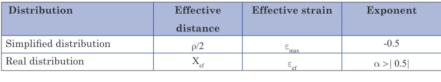
The strain distribution is characterized (in zone II) by three elements: the effective distance, X_ef, the effective strain e_ef and the exponent of the power law distribution a. In the past simplified strain distribution has been proposed (Fig.22).

The major elements of the strain distribution in a log-log chart are given in Table 3. The notch ductility factor (NDF)from Randall and Merkle [32] is the product of the maximum critical strain and the square root of the notch radius:

F_{R M−} =ε_{max c,} ρ

(

mm

)

₍₅₀₎

r is the defect tip radius and e_max,c the critical maximum strain. Similarly, from the real strain distribution the NDF can be defined as:

F=ε_{ef c,}

( )

X_ef α

( )

mm α (51)

One note that the Randall and Merkle notch ductility factor at the of leads to higher values than Fig.23. The values are however sensitive to the geometry and in particular to the ligament size.

9. SBD based on CDF versus strain or displacement curve

Crack driving force (CDF) represents the energy release rate when a crack emanating from a defect propagates by a small increment da. By a simple energy balance, it represents also the material force or fracture toughness. In fracture mechanics, several CDF are used: the elastic energy release rate G, the J integral and the crack tip opening displacement (CTOD). Due to the fact that SBD is used only in the case where the strains overcome the yield strain, only J and CTOD are used in a CDF-SBD. The Helmoltz free energy P is defined as:

P= −U P d. (52)

where U is the stored energy and P the external load. According to the above-mentioned definition, CDF is given as the derivative of P with respect to crack increment:

Distribution Effective

distance

Effective strain Exponent

Simplified distribution _{r/2 e}

max -0.5

Real distribution Xef e_ef a > | 0.5|

Fig.23. Comparison between F_{R M−} = ε_{max c,} ρand

F=ε_{ef c,}

( )

X_ef α, CT specimen.

Fig.25. CTOD design curve. Fig.24. The EnJ curve [34].

CDF P

a =−∂

∂

� ₍₅₃₎

Rice [33] has demonstrated that CDF can be presented as a contour integral called J:

J W dy T u x dS

i i

= − ∂

∂ 

   



   

∫



*

(54)

where S is the contour defined in a x, y coordinate system, W* is the strain energy density, T represents the traction forces and u_i the displacements. Crack tip opening displacement (CTOD) is the displacement at the original crack tip and the 90° intercept.

The principle of CDF-SDB is simple: the crack driving force is plotted versus the non-dimensional displacement d⁄d_y or non-dimensional net strain e_N /e_{N y,} where d_y and e_N,y are respectively displacement and net strain at yield load. CDF curve exhibits a parabolic part below yield load and linear above. Fracture toughness as critical CDF (CDF_c) is related to the upper limit of this curve. At the admissible strain e_ad corresponds the admissible CDF (CDF_ad). The difference between CDF_c and CDF_ad gives the safety margin.

9.1 Strain-based design based on J integral The J-SBD curve is based the relationship between the non-dimensional applied J integral and the dimensional displacement or non-dimensional net strain:

J E

a

f d

d

J E

a f

y y

y

N N y

.

.

.

. ,

σ

σ

ε

( )

=



  



  

( )

=



  

2

2 _



  

(55)

yield is G_y:

σ

π

y a y

E

G

( )

2 ₌ 2

.

(56)

Curves according to Equn 51 are sensitive to structure or component geometry and loading mode. Turner [34] has proposed a series of design curves based on the lower bound of different curves associated with different geometry as:

J E a d d for d d J E a

y y y

y . . . . σ π σ

( )

=         ≤

( )

= 2 2 2 2 2 1.. . .

254π 0 75 2

σ d d for d d J E y y y        −           ≤

(( )

=         ≤

( )

2 2 2

2 1 0

. . . , , a for J E N N y N N y y π ε ε σ   .. . . , a for N N y N N =        −          

1 254π 2ε 1 0 ε

  _,,y>1

(57)

A revised formula has been proposed by Turner in 1981 (34):

J G_y N N y ef N y = _, . . _,         +         ε ε   2

1 0 5

22

2

1 2

2 5 2

            ≤

( )

=  . . . . , , for J E a N N y y ef N y ε σ ε         −           >

2 0. 1 2.

, for N N y ε  (58)

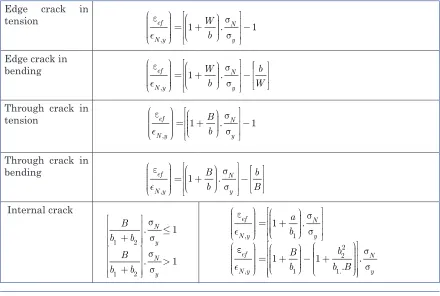
The effective strain on ligament is relatively complex to define. Turner has given [34] values of some non-dimensional effective strain which are resume in Table 4, where B is the specimen thickness, b₁ the smallest defect depth, b₂ the greatest defect depth.

9.2 Strain-based design based on CTOD

The crack tip opening displacement (CTOD) d is the displacement at the original crack tip and the 90° intercept. It measures the resistance of a material to crack initiation for materials that exhibits some plastic deformation before failure occurs causing the tip to stretch open. The strain base design using critical CTOD (d_{c) is used to determine the admissible defect size aad.}

This admissible defect size is given by the linear fracture mechanics on the lower part of the design curve and related to the critical stress intensity factor K_IC:

a_ad KIc

g D =         . , 1 2

where s_g,D is the design gross stress. For the upper part of the CTOD-SDB, the design curve is given as a function of the critical crack tip opening displacement :

a_ad c

y _{D y}

=         

₍

₎

−   . . / 1 2 1 1 π δ

ε _{ε ε} (60)

e_D is the design strain, and Equn 2 is valid for ferritic materials. For other materials, it is replaced by:

a_ad c

y D y =                

.1 . 2 2 π δ ε ε

ε (61)

In BS 7910 [35], the design curve is presented through the constant C. The admissible defect size can be written as:

a C K

a C ad Ic y ad c y =         =         . . σ δ ε 2 (62) Edge crack in

tension

Edge crack in bending

Through crack in tension

Through crack in bending Internal crack ε σ σ ef N y N y W b  _, .        = +                  − 1 1 ε σ σ ef N y N y W b b W  _, .        = +                  − 1         ε σ σ ef N y N y B b  _, .        = +                  − 1 1 ε σ σ ef N y N y B b b B  _, .        = +                  − 1         B b b B b b N y N y 1 2 1 2 1 1 . . +           ≤ +           > σ σ σ σ ε σ σ ef N y N y a b  _, .        = +                   1 1 εε_ef N y B b b b B  _{, .}.        = +        − +    1 1 1 22 1                . σ σ N y

C forC

g y

g y

=

(

)

=

(

)

≤

1

2

0 5

2

π σ σ

σ σ

/

/ .

(63)

C forC

g y

g y g y

=

(

)

−



 

=

(

)

≅

(

)

>

1

2π ε /ε 0 25. σ /σ ε /ε 0 5.

(64)

Equn 60 is limited to ferritic steel. For other materials Equn 61 is used.

C forC

g y

g y g y

=

(

)

=

(

)

≅

(

)

>

1

2

0 5

2

π ε ε

σ σ ε ε

/

/ / .

(65)

The CTOD design curve is presented in Fig.25. However more conservative values of constant C have been introduced [36].

10. Conclusion

Defect Aasessment Procedures within SBD exhibits FOUR types of approach:

• a gross strain criterion;

• a critical local strain approach;

• criteria base on strain distribution at defect tip; • criteria based on CDF versus strain or displacement.

They are above described but due to the large variety a method to choose the appropriate one is necessary.

The choice can be made: (i) according to the degree of conservatism, (ii) independence to geometry and loading mode, and (iii) facility to implement. One does not take into account the notch ductility factor (NDF) which is relatively ancient and not used. It has been cited in this paper for historical point of view. The SBD curves associated with CDF are strongly conservative because this curve has been obtained as the lower bound of different results from specimen with different geometries and loading mode. This approach is easy to use and found in codes and Fracture toughness as JIC and Critical COD can be found easily in data based. SBD using strain distribution at notch tip needs finite element methods particularly in 3D if one intends to take into account out of plane constraint. Effect of geometry and loading mode can be considered using constraint described by Q parameter or stress triaxiality and two parameters fracture mechanics. In this case, one reduces strongly the conservatism, but the analysis is rather complex. This approach needs to establish the material failure master curve which is obtained with a least four different failure tests on different specimens. The local strain approach needs to use the same method i.e. the finite element method. Structure geometry and loading mode is taken into account through stress triaxiality and lode angle. Here, conservatism is relatively limited but the use of Xu and Wierbiecki model of critical strain needs experimental identification of four parameters with mixed loading mode.

The critical gross strain criterion is obtained experimentally by full thickness tensile test. This needs generally high capacity testing machine and test are relatively expensive. Tests in real situation avoid conservatism.

Conflicts of interest

The author has no conflicts of interest to declare.

References

[1] DNV 2000. DNV-OS-F101 Submarine pipeline systems, det Norske Veritas. [2] CSA. 1999. Z662 Oil and gas pipeline systems, Canadian Standards Association.

[3] ASME, 2012. B31.8, Gas transmission and distribution piping systems. American Society of Mechanical Engineers. New York.

[4] API 1104, 1999. Welding of pipelines and related facilities, 19th _{Edn, American Petroleum Institute.} [5] API, 1998. RP 1111 Design, construction, operation and maintenance of offshore hydrocarbon

pipelines limit state design), American Petroleum Institute.

[6] BSI, 1000. BS7910:1999, Guide on methods for assessing the acceptability of flaws in metallic

structures, British Standards Institution.

[7] F.A. MacClintock, 1998. A criterion for ductile fracture by the growth of holes. Journal of Applied

IMechanics 35, 363.

[8] J.W. Hancock and A.C. MacKenzie, 1976. On the mechanisms of ductile failure in high-strength steels, Journal of Mech. Physic. of Solids, 24, 147-169.

[9] D.Holland, A. Hallen, and A. Dahl, 1990. Steel Research, 504-506.

[10]. A. Dhiab, H. Gouair, Z. Azari, G. Pluvinage, 1996. Dynamic ductile failure of xc18 steel: statistical aspects, Problems of Strength, Special Publication 96, 38-46.

[11] J.R. Griffith. and D.R.J. Owen, 1972. Journal of Mechanics and Physics of Solid, 19, p 419.

[12] J.R. Rice and D.M. Tracey, 1969. On the ductile in triaxial stress fields, Journal of Mechanics and

Physics of Solids ,26, 163-186.

[13] J.T. Barnby et al., 1984. On the void growth in C-Mn structural steels during plastic deformation. Int

Journal of Fracture, 25, pp 271-284.

[14] J.A. Lemaitre, 1985. Continuous damage mechanics model for ductile fracture. J Eng Mater Technol,

107, 83–89.

[15] N.A. Bonora, 1997. A nonlinear CDM model for ductile failure. Engineering Fracture Mechanic, 58,

Issues 1–2, September: 11-28.

[16] Y. Bao and T. Wierzbicki, 2004. On fracture locus in the equivalent strain and stress triaxiality space.

International Journal of Mechanical Sciences, 46, Issue 1, January, 81–98.

[17] K. Nahshon and J.W. Hutchinson, 2008. Modification of the Gurson model for shear failure. European

Journal of Mechanics-A/Solids, 27 (1) 1–17.

[18] T. Wierzbicki and L. Xue, 2008. Ductile fracture initiation and propagation modelling using damage plasticity theory. Engineering Fracture Mechanics, 75, 3276-3293.

[19] R. Denys, 2007, Interaction between material properties, inspection accuracy and defect acceptance levels in strain based pipeline design. Safety, reliability and risks associated with water, oil and gas pipelines, Eds G. Pluvinage and M. Elwany, Springer. pp 1-22.

[20] H. Gouair, Z. Azari, D. Cicliov, and G. Pluvinage, 1995. Ténacité d’un matériau ductile ; un modèle

basé sur la distribution locale critique de la déformation. Matériaux et Techniques, 12, 7-12.

[21] R.J. Eiber, 1981. The effect of dents on the failure characteristics of linepipe, Batelle Colombus Laboratories. NG 18, Report N° 125, May.

[22] D.G. Jones, 1982. The significance of mechanical damage in pipelines, 3R International, 21, Jahrgang, Heft.

[23] API, 2000. Fitness-for-Service. API Recommended Practice 579, 1st Edn, American Petroleum Institute; January.

[24] P. Roovers, R. Bood, M. Galli, U. Marewski, M. Steiner, and M. Zarea, 2000. EPRG methods for assessing the tolerance and resistance of pipelines to external damage, Pipeline Technology, Volume II, Proceedings of the Third International Pipeline Technology Conference, Bruges Belgium, R. Denys, Ed., Elsevier Science:405-425.

[25] A.K. Escoe, 2006. Piping and pipelines assessment guide. Volume I, British Library Cataloguing-in-Publication Data, Elsevier.

[27] M. Allouti, C. Schmitt, and G. Pluvinage, 2014. Assessment of a gouge and dent defect in a pipeline by a combined criterion, Engineering Failure Analysis, 36, January, 1–13.

[28] M. Oyane, T. Sato, K. Okimoto, S. Shima, 1980. Criteria for ductile fracture and their application, J.

Mech. Work Technol. 4.

[29] M. Allouti, C. Schmitt, G. Pluvinage, J. Gilgert, and S. Hariri, 2012. Study of the influence of dent

depth on the critical pressure of pipeline, Engineering Failure Analysis, 21, 40-51, April.

[30] Russian code M-02-91, 1991. Method to determine the admissible defect size in pipes and components of nuclear power plant, in Russian. Steel, Journal of Engineering for Industry, 935-941, August. [31] J .R. Rice, 1968. Journal of Applied Mechanics, 35, 379/386.

[32] C.E. Turner, 1981. The J estimation curve, R curve, and tearing resistance concepts. Fitness for purpose validation of welded constructions. Paper 17, Weld. Inst., Cambridge.

[33] BSI 1999. BS7910 Guidance on methods for assessing the acceptability of flaws in fusion welded

structures.

[34] G. Pluvinage, Y. Lecointe, and F. Montariol 1974. Application de la mécanique plastique des ruptures à la prévision de la taille de défaut critique, Journal de Physique, Juillet.