Artificial Neural Network to Construct a Pattern Recognition System for Inspecting Fabric Fefects

(1)

Artificial Neural Network to Construct a Pattern

Recognition System for Inspecting Fabric Defects

P. Satyanarayan

Dept. of Mathematics & Computer Science , Osmaniya

University, Hyderabad, Telangana, India

M. V. Ramana Murthy

Srikanth Nivathi

B. Chithra

Abstract – In this paper, we evaluate the efficiency and

accuracy of a method of detecting fabric defects that have been classified into different categories by a neural network. Four kinds of fabric defects most likely to be found during weaving were learned by the network. Based on the principle of the back-propagation algorithm of learning rule, fabric defects could be detected and classified exactly. The method used for processing image feature extraction is a co-occurrence-based method, by which six feature parameters are obtained. All of them consist of contrast measurements, which involve three spatial is placements (i.e., 1, 12, 16) and four directions (0, 45, 90, 135 degrees) of fabric defects’ images used for classification. The results show that fabric defects inspected by means of image recognition in accordance with the artificial neural network agree approximately with initial expectations.

It has become more and more important for textile engineers to use automatic techniques in production processes and management procedures. At present, fabric inspection still depends on human sight, and inspection results are greatly influenced by the mental and physical condition of an inspector. To economize on personnel and to increase the competitive ability of products it is necessary to automate the inspection of fabric defects during weaving.

In this study, we use a neural network topology known as “multi-layer perception,” which has not been used in the past because of the lack of effective training algorithms for it. Recently this has changed due to the development of an iterative gradient procedure known as the back-propagation algorithm [7]. Through this supervised learning algorithm, the neural network can become a classifier of fabric defect Because of the highly parallel operation and quick response nature of a neural network, it is easy to apply this method to on-line monitoring of fabric defects in weaving.

Keywords – Neural Networks, Knitted Fabrics, Sigmoid

Transfer Function, Textile, Pattern Recognition.

I. E

XTRACTING

F

EATURE

P

ARAMETERS OF

A

F

ABRIC

D

EFEATS

T

EXTURE

Texture may be defined with respect to the global properties of an image or to the repeating units that compose it. In this paper, we use a gray level co-occurrence matrix [1, 4, 9] to extract various feature parameters of a fabric defect’s texture image to evaluate defects in various categories.

Texture Image, regarded as a two-dimensional function of light intensity, can be illustrated as a function f(x, y). For each coordinate (x, y) (or pixel-x, y) in a two-dimensional image, there is a corresponding function value of light intensity. Because the image exists in an energy form [2], the magnitude of function f(x, y) for the

image can be any value except zero and can be shown as 0 < f (x, y) < ∞.

Generally speaking, the reason the image of an object can be observed by human vision is the light intensity reflected from it, which consists of two parts, the light intensity illuminating the object itself and the light intensity reflected from the surface of the object. The former is illumination, represented by i(x, y), and the latter is reflectance, represented by r(x, y), The image of an object can thus be shown using Equation 1:

F(x,y) = i(x,y)r(x,y) (1)

Where 0< i(x,y)< ∞ and 0 < r(x,y)<1

The magnitude of r(x, y) is between 0 (indicating no reflection from the surface of an object) and 1 (indicating full reflection from the surface). The magnitude of reflectance r (x, y) depends on the light intensity reflected from the surface of the object.

In order to permit a continuous spatial image, function f(x, y) for the image through digitized processing becomes a discrete spatial function. This process is called “image sampling”. Every pixel of an image can then be represented as f(x, y), and the N X N size of image in its digital form can be stored as a two-dimensional array using Equation 2:

F(x,y)

f(0,0) f(0,1) … f(0, N – 1) f(1,0) F(1,1) … f(1, N – 1) = … … … … … … … …

F(N – 1,0) f(N- 1,1) … f(N – 1,N – 1) (2) This digital image f (j, k) is N X N, and its gray level resolution is G. We used two parameters-d, the distance between two pixels, and θ, the position angle between two pixels (j, k) and (m, n). Thus, there were four directions of position angle-the horizontal direction θ = 00, the right diagonal direction θ = 450, the vertical direction θ= 900, and the left diagonal direction θ = 1350. The four kinds of relative positions between two pixels can be dented using Equation 3:

θ = 00 R(d) : |j – m| = d, k – n = 0

θ = 450 R(d): (j – m = - d, k – n = -d) Or (j – m = d, k – n =d)

θ = 900 R(d): j – m = 0, | k – n | = d

θ = 1350 R(d) : (j – m = -d, k – n = d)

Or (j – m = d, k – n = - d) (3) Based on this definition, the relationship between the pixel pairs and the co-occurrence probability of gray levels p and q can be illustrated using Equation 4

(2)

= # {RRD (d), f(j,k) = p, f(m,n) = q} P (p,q,d, 900)

= # { Rγ (d), f(j,k) = p, f(m,n) =q}

P(p,q,d, 1350) = # {RLD (d), f(j,k) = p, f(m,n) = q} (4) The symbol # { } denotes the probability sum of occurrence of all events in the parentheses. P is a function of four parameters p, q, d, θ. As for an image of gray level 0-3, its co-occurrence matrix is illustrated in Figure 1 a. An image size of 4 X 4 is illustrated in Figure 1 b, and each co-occurrence matrix of direction 00, 450,900, 1350 is shown in Figures 2a, b, c, and d.

Fig. l. (a) General form of co-occurrence matrix for image with gray level 3 (b) 4 x 4 image with four gray level

0-3 and the arrows show four direction angles of position between two pixels

PN (d=1, θ = 00) =

















4

0

6

0

1

0

4

2

0

4

PRD (d=1, θ = 450)

=

















0

3

0

2

3

0

4

1

2

0

1

2

(b)

PV (d=1, θ = 900) =

















0

3

1

2

3

0

1

0

1

6

0

2

0

4

PLD (d=1, θ =

1350) =

















0

2

1

2

0

1

0

2

1

2

1

0

1

2

(c) (d)

Fig. 2. (a-d) illustrate calculations of four direction angles of position in co- occurrence matrix.

A co-occurrence matrix is processed using the normalization method [6, 9] to make the sum of all the entries in the matrix equal to 1. Then the ASM (angular second moment), the parameter for the evenness distribution degree of the image, and CON (contrast), the

parameter for the gray level contrast of the image, are obtained using Equations 5 and 6:

( )













=

∑

R

q

p

P

ASM

q p

2

,

(5) and

( )





























=

∑

= − −

=

R

q

p

P

S

CON

s q p m

n

,

1

0 2

(6) where R denotes the sum of all the entries of the co-occurrence matrix.

II. C

ONSTRUCTION AND

T

RAINING OF

T

HE

N

EURAL

N

ETWORK

A network consisting of one input layer, one output layer, and one hidden layer is used in the pattern recognition system of fabric defect texture in this study. Its construction is illustrated in Figure 3.

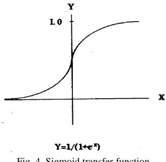
Fig. 3. A multi-layer perceptron with one hidden layer “Training” is equivalent to finding proper weights for all the connections of nodes between layers such that a desired output is generated for a corresponding input. The major training steps of the back propagation algorithm are as follows [3, 7, 8, 11]: (a) Initialize all the values of connection weight (Wijs) between node j in the upper layer and node i in the layer below. (b) Present an input for each node in the input layer and specify the desired output for each node in the output layer. (c) Calculate actual outputs of all the nodes using the present value of Wijs. The output of node j, denoted by YJ, is a on linear function (called a Sigmoid function and shown in Figure 4) of its total input: Yj =

ij

net

e

−

+

1

(7)

where netij = ij i

i

W

Y

∑

. (d) Find an error term for each

output node and hidden node. If dJ and YJ stand for desired and actual values of a node, respectively, for an output node,

δJ = (dJ – YJ) Yj(1 –YJ) (8) and for a hidden layer node,

δJ = Yj(1 –YJ) ij k

k

W

(3)

Update weights by Wij(t +1) = Wij(t) + αδJ Yt

+ γ(Wij (t) – Wij (t – 1)) (10) where Wij (t) stands for connection weight value between node j in the upper layer and node i in the layer below, α is a learning rate, and the momentum factor γ is a constant between 0 and 1. (f) Return to step b to present another new input for each node until all the training sets have been learned and the weights have stabilized.

Fig. 4. Sigmoid transfer function

III. E

XPERIMENTAL

Samples And Image Capture

The fabrics used in this study were twills woven by T / W warp and T / W weft, which are both folded yarns. In addition to these normal fabrics, there were various kinds of defective fabrics with neps, broken ends, broken picks, and oil stains, all of which appear fairly often during weaving. The characteristics of the normal fabrics are shown in Table I. From each of the four kinds of defective fabrics, ten samples were taken by image capture equipment and randomly divided into two groups. One half was used for training and the other half for testing.

Table 1. Characteristics of normal fabrics. Tex Density, yarn/in. Material

Warp 30 92 T/W(folded yarn)

Weft 30 42 T/W(folded yaren)

The image capture system is shown in Figure 5. Images were captured using a panasonic CCD camera (Solid Color WV-CD 110) equipped with a 20X lens. Each image was digitized by Ip-8/AT card into 100 X 100 pixels with a gray level of 0-255 and stored as a Two-dimensional array. Samples were illuminated by two halogen lights positioned approximately 20 cm above and to the right and left of the sample to supply illumination in diagonal directions of 450. Captured images could be reproduced on the graphic display, whose resolution power was 320 X 200 with a gray level range of 0-255. The feature parameters of each fabric defect’s texture were calculated by an IBM personal

computer with CPU 486 DX-50.

Fig. 5. Schematic illustration of the inspection system

IV. P

ROCEDURES

Gray Scale Histogram Equalization Preprocessing There are two reasons to use the histogram equalization processing method [5, 6] to reduce a 256 gray level resolution of the image to a 16 gray level. The first reason is to conserve computation time and the second is the recognition that human vision is commonly below the 16 gray level.

Through histogram equalized processing, we obtained a more uniform gray level distribution of the images, thus avoiding varied results from image capture conditions.

Acquiring the Repetition Units of Normal Fabrics Using reduced image data, the co-occurrence matrix for a normal fabric’s texture image can help determine the repetition distance d along a direction angle of θ. If the intensity distribution of all the pixels in an image is a normal distribution, the angular second moment (ASM) and contrast (CON) [1, 4, 9] can be calculated using Equations 5 and 6.

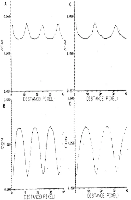
Regardless of the kinds of direction, if there is any periodicity in the direction of θ, the diagonal elements in a co-occurrence matrix become large values [4, 9]. Thus, the value of ASM in Equation 5 becomes the maximum and the value of CON in Equation 6 becomes the minimum. Figure 6 illustrates ASM and CON statistics plotted against d for 00 and 900 directions. The figure reveals that the periodic signals in normal fabrics are strongest in the horizontal and vertical directions (weft and warp). The maximum ASM and the minimum CON at the distance of 12 pixels (d = 12) along the horizontal direction (θ = 00) are shown in Figures 6A and B, respectively, and those at a distance of 16 pixels (d = 16) along vertical direction (θ = 900) are illustrated in Figures 6C and D, respectively. Thus, of the normal fabrics, the repetition unit along the weft direction is 12 pixels and that along warp direction is 16 pixels.

(4)

0

) f2 =CON(d= 1, θ = 45 0

), f3 =CON(d= 1, θ = 900), f4 =CON(d= 1, θ = 1350), f5 =CON(d= 12, θ = 00), and f6 =CON(d= 16, θ = 900).

Training and Testing Sets Having obtained the feature parameters for fabric defects, the next step is to generate training and testing sets. From each of the four kinds of defective fabrics and the normal fabrics, ten samples were taken with image capture equipment, and the samples of each kind of fabric defect (including the normal fabrics) were

Fig. 6. Results of ASM and CON with the change of distance at being equal to 00 and 900 (A) ASM (θ = 00) (B)

CON (θ = 00) (C) ASM (θ = 900) (D) CON (θ = 900) Randomly partitioned into two sets. One was used for training, shown in Table II, and the other for testing, shown in Table III.

V. N

EURAL

N

ETWORK

A

RCHITECTURE

In this paper, we used a back-propagation neural network to develop a classifier of fabric defects. Using a software package called Professional II / PLUS [10] , we tried different network topologies: a 6-12-5 network gave the best results. The input consisted of six input nodes corresponding to the number of feature parameters. A hidden layer of twelve nodes fed into the output layer of five nodes, representing the five kinds of fabric defects (including the normal fabrics). Learning rate and momentum factor were 0.5 and 0.4, respectively. For this study, we used a Sigmoid transfer function.

VI. R

ESULTS AND

D

ISCUSSION

Selecting Feature Parameters

Each kind of defect found on a certain area of a fabric will result in a different texture from that of the normal fabrics. The textures of different kinds of fabric defects should be different from each other as well.

Based on the point of view mentioned above, a good feature should satisfy two requirements. The first is that those that are slightly different textures with similar general characteristics should have numerically close feature values, and the second is that the features from different classes should be quite different numerically from each other. Furthermore, in order to conserve computation time, it is necessary to find a set of numerical features (a feature vector) whose dimensions are much lower than the original data of texture imaging.

The degree of success of an inspection system heavily depends on how adequate, general, and compact the representation of each kind of fabric defect is. For instance, each texture of the normal fabrics and the four kinds of defective fabrics are illustrated in Figure 7A.

Through human vision, the textures of both normal and defective fabrics can easily be classified, but when applying the pattern recognition technique to classification of fabric defects, it is essential to extract some good feature parameters mentioned above.

Table 2. Training set for various kinds of fabric defects. Fabric

defects

Input vector, f1, f2, f3, f4, f5, f6 Output

vector

Normal 1 2 3 4 5

(.3978,.6433,.3704,.4430,.3584,.3811) (.3920,.6464,.3532,.4221,.3352,.3859) (.3887,.6363,.3601,.4202,.3220,.3257) (.3880,.6322,.3672,.4302,.3481,.3378) (.3851,.6228,.3567,.4361,.3496,.3371)

(1,0,0,0,0) (1,0,0,0,0) (1,0,0,0,0) (1,0,0,0,0) (1,0,0,0,0)

Nep 1

2 3 4 5

(.3529,.5768,.3219,.3865,.4417,.4725) (.3465,.5874,.3225,.3819,.4740,.5255) (.3467,.5767,.3130,.3782,.3845,.4925) (.3697,.5805,.3232,.3978,.4660,.4953) (.3537,.5642,.3182,.3918,.4358,.5035)

(0,1,0,0,0) (0,1,0,0,0) (0,1,0,0,0) (0,1,0,0,0) (0,1,0,0,0)

Broken end

1 2 3 4 5

(.3159,.5158,.3214,.3981,.5433,.3301) (.3354,.5356,.3373,.4095,.5594,.3677) (.3231,.5202,.3197,.3899,.5466,.3510) (.3535,.5655,.3275,.4129,.5210,.3302) (.3761,.5795,.3399,.4324,.5290,.3305)

(0,0,1,0,0) (0,0,1,0,0) (0,0,1,0,0) (0,0,1,0,0) (0,0,1,0,0)

Broken pick

1 2 3 4 5

(.3765,.6080,.3098,.3842,.3198,.3578) (.3987,.6132,.3145,.3954,.3272,.3829) (.3840,.5953,.3123,.3920,.3165,.4022) (.3854,.6023,.3101,.3890,.3154,.3635) (.3873,.5970,.3074,.3944,.3554,.3735)

(0,0,0,1,0) (0,0,0,1,0) (0,0,0,1,0) (0,0,0,1,0) (0,0,0,1,0)

Oil stain

1 2 3 4 5

(.3592,.4453,.3003,.3543,.4673,.4100) (.4049,.4874,.3207,.3977,.5187,.4240) (.3586,.4805,.3102,.3614,.4967,.8066) (.3049,.3866,.2726,.3215,.4967,.5492) (.4029,.5257,.3363,.4028,.5465,.4661)

(5)

Fabric

defects Input vector, f1, f2, f3, f4, f5, f6

Output vector

Normal 1 2 3 4 5

(.3900,.6402,.3584,.4205,.3726,.3434) (.4026,.6362,.3601,.4320,.3438,.3442) (.3879,.6161,.3419,.4153,.3228,.3547) (.3931,.6381,.3569,.4284,.3694,.4308) (.3826,.6298,.3537,.4234,.3489,.3435)

(1,0,0,0,0) (1,0,0,0,0) (1,0,0,0,0) (1,0,0,0,0) (1,0,0,0,0)

Nep 1 2 3 4 5

(.3689,.6188,.3483,.4026,.4393,.4813) (.3789,.6173,.3447,.4042,.3954,.4213) (.3663,.6173,.3444,.4045,.4439,.4788) (.3881,.6345,.3569,.4305,.4214,.5121) (.3964,.6362,.3512,.4236,.4049,.4210)

(0,1,0,0,0) (0,1,0,0,0) (0,1,0,0,0) (0,1,0,0,0) (0,1,0,0,0)

Broken end

1 2 3 4 5

(.3509,.5957,.3507,.4079,.5432,.3107) (.3661,.5915,.3361,.4137,.4808,.2884) (.3717,.5968,. 237,.4003,.4708,.3376) (.3589,.5903,.3230,.3931,.4377,.3266) (.3436,.5775.3298,.3907,.4888,.3454)

(0,0,1,0,0) (0,0,1,0,0) (0,0,1,0,0) (0,0,1,0,0) (0,0,1,0,0)

Broken pick

1 2 3 4 5

(.3723,.5821,.2097,.3695,.3453,.3765) (.3836,.6022,.3054,.3861,.3383,.3429) (.3716,.5918,.3101,.3761,.3595,.3248) (.4115,.6037,.2797,.4036,.3987,.3294) (.4321,.6446,.3090,.4157,.4254,.3284)

(0,0,0,1,0) (0,0,0,1,0) (0,0,0,1,0) (0,0,0,1,0) (0,0,0,1,0)

Oil stain

1 2 3 4 5

(.4000,.4976,.3254,.3969,.5242,.4233) (.2626,.3115,.2417,.2633,.4584,.3841) (.2657,.3276,.2263,.2723,.3681,.4321) (.3640,.4823,.3034,.3518,.5274,.6200) (.4051,.5158,.3361,.4082,.6228,.6095)

(0,0,0,0,1) (0,0,0,0,1) (0,0,0,0,1) (0,0,0,0,1) (0,0,0,0,1)

Haralick et al. [4] proposed a variety of measures that can be applied to extract useful information from a co-occurrence matrix. Among them, contrast (CON), which is a measure of the amount of local variation present in an image, is able to characterize each kind of fabric defect. First, we extracted CON measures along four directions of each sample defect (f1 f2, f3, f4) from the co-occurrence matrix to characterize each defect. To promote the correct classification rate in fabric defects, apart from f1- f4 feature parameters (CON measures along 00, 450, 900, 1350, respectively), we extracted two more feature parameters f5 and f6 by

Fig. 7. (A) A 100 x 100 digitized sample of each texture of normal fabrics and various kinds of defective fabrics, from

top and from left to right Normal, Nep, Broken End, Broken Pick, Oil Stain (B) Samples of various textures of Broken End fabric defect determining the repetition units of normal fabrics along the horizontal (d = 12) and vertical

directions (d = 16)

In Tables II and III, broken ends have a large f5 value and a small f6 value while broken picks have a small f5 value and a large f6 value. From these two feature parameters, we obtained a more specific feature vector for classifying different fabric defects.

Using the gray level co-occurrence matrix [9], we obtained six feature parameters for each kind of fabric defect to represent the original image data and conserve computation time.

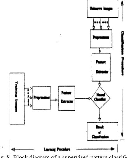
Artificial neural networks (ANNs) are capable of many functions, among them, clustering, mapping, optimization, and classification [3, 7, 11]. In this study, we used the network as a supervised classifier, which is a decision-making process that requires the network to identify the category best representing an input fabric defect texture pattern. The identifying method is outlined in a block diagram shown in Figure 8.

Accuracy and Efficiency of Recognition

In the past, the traditional technique of pattern recognition has been pattern matching, which was easily affected by noise, thus ruining its accuracy. In addition to a highly parallel operation and quick response, artificial neural networks also have the advantage of fault tolerance. Some samples of broken end defective fabric texture used for the ANN classifier in the testing process are shown in Figure 7B. These samples, whose textures differ somewhat from each other, can still be accurately

.

Fig. 8. Block diagram of a supervised pattern classi6cation scheme

Classified by an ANN. The results in Table IV show that the accuracy rate of classification is as high as 9696.

VI. C

ONCLUSIONS

(6)

DX-50. Classification of texture takes only a fraction of a second, and the main computational requirements of an ANN occur during its training process, which can be performed off line. Thus a pattern recognition system in accordance with ANN is a pretty good classifier for on-line monitoring of fabric defects in weaving. Through the feature vector consisting of f1-f6, we obtained an adequate, general, compact representation for each kind of fabric defect. The detection process uses the learning capacity and fault tolerant nature of the artificial neural network. Through the supervised learning algorithm of back-propagation, the neural network can become a good classifier for fabric defects. Experiments on various kinds

of fabric defects have yielded satisfactory results.

Table 4. results of discrimination Output vector Fabric

defects

Desired Actual Result

a Normal 1.0000 0.0000

0.0000 0.0000

0.0000

1.0000 0.0000

0.0000 0.0000

0.0000

1.0000 0.0000

0.0000 0.0000

0.0000

1.0000 0.0000

0.0000 0.0000

0.0000

1.0000 0.0000

0.0000 0.0000

0.0000

.8702 -.0009

.1220 .1920 -.0719

.8695 -.0872

.0310 .1364 -.0144 .6864 .0482 .0305 .3440 -.0425 .7691 .3082 .0240 .0276 -.0305

.8926 -.0119

.1027 .0929 -.0978

a

b Nep 0.0000 1.0000

0.0000 0.0000

0.0000

0.0000 1.0000

0.0000 0.0000

0.0000

0.0000 1.0000

0.0000 0.0000

0.0000

0.0000 1.0000

0.0000 0.0000

0.0000

0.0000 1.0000

0.0000 0.0000

0.0000

.3621 .9855

.0410 .0860 -.0500

.5032 .5480

.0105 .0575 -.0323 .3290 .9864 .0303 .0852 -.0143 .4976 .3945 .0303 .0852 -0143

.5702 .3883

.0172 .0474

.0125

b

a

c Broken end

0.0000 0.0000

1.0000 0.0000

0.0000

0.0000 0.0000

1.0000 0.0000

0.0000

0.0000 0.0000

1.0000 0.0000

0.0000

0.0000 0.0000

1.0000 0.0000

0.0000

0.0000 0.0000

1.0000 0.0000

0.0000

.2836 .0608

.9740 .1652 -.0944

.4335 -.0585

.7560 .0243 -0698

.1497 .2615

.4264 .0836 -.0050

.3042 .2271

.4039 .1125 -.0826

.2061 .3798

.6699 .0916 -.0891

c

d Broken pick

0.0000 0.0000

0.0000 1.0000

0.0000

0.0000 0.0000

0.0000 1.0000

0.0000

0.0000 0.0000

.1797 .1930

-.1656 1.0738

.0587 .0065 .0219 .0168 .7517 -0220 .1065 .0219

-d

d

0.0000 1.0000

0.0000

0.0000 0.0000

0.0000 1.0000

0.0000

0.0000 0.0000

0.0000 1.0000

0.0000

.0168 .7517 -.0220 .2638 .1321

-.1475 1.1967

.3523 -.1228-.0753 .9525 .3247

d

e Oil stain 0.0000 0.0000

0.0000 0.0000

1.0000

0.0000 0.0000

1.0000

0.0000 0.0000

1.0000

0.0000 0.0000

1.0000

0.0000 0.0000

1.0000

-.2423 -.0469

.1050 .0059

.9123 -.3212 -.2341

.2157 .4036

.9373 .3265 .1196

-.1484 1.0740

.7956 .2833 .0021

-.0453 .0104

1.0243 -.2618 -.1154

.1674 -.1871

1.0614

e

d

e

R

EFERENCE

[1] Don, H. S., Fu, K. S., Liu, C. R., and Lin, W. C., Metal Surface Inspection Using Image Processing Techniques, IEEE Trans. Sys. Man Cybernet. SMC-14 (1), 139-146 (1984).

[2] Gonzalez, R. C., and Woods, R. E., "Digital Image Processing,"

Addision-Wesley Publishing Co., NY, 1992.

[3] Gou, L. C., "Theory of Neural Net System," Zoo-Lin Publishing

Co., Taipei, R.O.C., 1991.

[4] Haralick, R. M., Shanmugam, K., and Dinstein, I., Texture

Features for Image Classification, IEEE Trans. Sys. Man Cybernet. SMC-3., 610-621 (1973).

[5] Khotanzad, A., and Kashyap, R. L., Feature Selection for

Texture Recognition Based on Image Synthesis, IEEE Trans. Sys. Man Cybernet. SMC-17 (6), 1087-1095 (1987).

[6] Lien, K. J., "Digital Image Processing," Zoo-Lin Publishing Co., Taipei, R.O.C., 1992.

[7] Lu, B. S., and Tsau, D. F., "Theory and Application of ANN," Chuan-Hua Technology Publishing Co., Taipei, R.O.C., 1992. [8] Nelson, M. M., and Illingworth, W. T., "A Practical Guide to

Neural Nets," Addision-Wesley Publishing Co., NY, 1991. [9] Sobus, J., Pourdeyhimi, B., Gerde, J., and Ulcay, Y., Assessing

Changes in Texture Periodicity Due to Appearance Loss in Carpets: Gray Level Co-occurrence Analysis, Textile Res. J. 61 (10), 557-567 (1991).

[10] "The Professional II/PLUS Neural Network Software User’s

Manual," NeuralWare, Inc., U.S.A., 1993.

[11] Yei, I. C., "Application and Practice of Artificial Neural Network Algorithm," Zoo-Lin Publishing Co., Taipei, R.O.C., 1993.

A

UTHOR

'

S

P

ROFILE

Dr. P. Satyanarayana presently working as a java and

integration Lead developer to the ministry of interior affairs at kingdom of Saudi Arabia. Awarded Ph.D. by Osmania University in the year 2014 in Neural networks applications to textile industry.

Prof. M. V. Ramana Murthy, Professor in department