www.geosci-model-dev.net/7/755/2014/ doi:10.5194/gmd-7-755-2014
© Author(s) 2014. CC Attribution 3.0 License.
Geoscientific
Model Development
Assessing the CAM5 physics suite in the WRF-Chem model:
implementation, resolution sensitivity, and a first evaluation for a
regional case study
P.-L. Ma1, P. J. Rasch1, J. D. Fast1, R. C. Easter1, W. I. Gustafson Jr.1, X. Liu2, S. J. Ghan1, and B. Singh1
1Atmospheric Sciences and Global Change Division, Pacific Northwest National Laboratory, Richland, Washington, USA 2Department of Atmospheric Science, University of Wyoming, Laramie, Wyoming, USA
Correspondence to: P.-L. Ma ([email protected])
Received: 26 September 2013 – Published in Geosci. Model Dev. Discuss.: 29 November 2013 Revised: 17 March 2014 – Accepted: 18 March 2014 – Published: 6 May 2014
Abstract. A suite of physical parameterizations (deep and
shallow convection, turbulent boundary layer, aerosols, cloud microphysics, and cloud fraction) from the global climate model Community Atmosphere Model version 5.1 (CAM5) has been implemented in the regional model Weather Re-search and Forecasting with chemistry (WRF-Chem). A downscaling modeling framework with consistent physics has also been established in which both global and regional simulations use the same emissions and surface fluxes. The WRF-Chem model with the CAM5 physics suite is run at multiple horizontal resolutions over a domain encompass-ing the northern Pacific Ocean, northeast Asia, and northwest North America for April 2008 when the ARCTAS, ARCPAC, and ISDAC field campaigns took place. These simulations are evaluated against field campaign measurements, satellite retrievals, and ground-based observations, and are compared with simulations that use a set of common WRF-Chem pa-rameterizations.
This manuscript describes the implementation of the CAM5 physics suite in WRF-Chem, provides an overview of the modeling framework and an initial evaluation of the sim-ulated meteorology, clouds, and aerosols, and quantifies the resolution dependence of the cloud and aerosol parameteri-zations. We demonstrate that some of the CAM5 biases, such as high estimates of cloud susceptibility to aerosols and the underestimation of aerosol concentrations in the Arctic, can be reduced simply by increasing horizontal resolution. We also show that the CAM5 physics suite performs similarly to a set of parameterizations commonly used in WRF-Chem, but produces higher ice and liquid water condensate amounts
and near-surface black carbon concentration. Further evalu-ations that use other mesoscale model parameterizevalu-ations and perform other case studies are needed to infer whether one parameterization consistently produces results more consis-tent with observations.
1 Introduction
The typical grid size for current GCMs is still rather coarse and ranges from 0.5 to 4 degrees for the atmosphere (Taylor et al., 2012). For example, the Community Atmo-sphere Model (CAM) version 5 (CAM5) (Neale et al., 2010), the atmospheric component of the Community Earth System Model (CESM) version 1 (Hurrell et al., 2013), typically uses a grid spacing of 1 to 2 degrees. GCMs are expected to take advantage of growing computational resources and run at much higher resolutions in the future. However, the applica-bility of climate model treatments of physical, chemical, and dynamical processes in a high-resolution setting has not been fully tested, and the resolution dependence of model physics and model biases is not well understood. Rapid development and evaluation of the next generation of CESM requires the ability to isolate processes as well as routinely test parame-terizations across a range of scales. Yet, it is computationally expensive to repeatedly conduct long (e.g., multi-year) high-resolution GCM experiments to explore these issues, even on the most powerful modern supercomputers.
The dynamical downscaling approach that uses a rela-tively high-resolution regional climate model (RCM) has been widely utilized to better represent and understand the climate system at local and regional scales (e.g., Leung and Ghan, 1999a, b; Leung and Qian, 2003; Leung et al., 2003a, b, 2004; Liang et al., 2006). RCMs often focus on repro-ducing real-world weather events (e.g., Liang et al., 2011; Lin et al., 2011; Ma et al., 2012; Yang et al., 2012), and they are usually run at much smaller grid spacings (e.g., 10 km) over a limited domain for a shorter period of time with high-resolution topography and lateral boundary con-ditions provided by a GCM or global analyses. Global and regional modeling communities have advanced their mod-eling techniques independently over the years, with differ-ent philosophies and goals. Because RCMs typically operate over smaller timescales and spatial scales, they can explic-itly resolve some physical processes that must be parameter-ized in GCMs. For example, when the Weather Research and Forecasting (WRF) model (Skamarock et al., 2008) is run at mesoscale or cloud-resolving resolutions that can explicitly resolve cloud updrafts, cumulus parameterizations and other subgrid cloud treatments are not required. Detailed spectral bin microphysics schemes can also be employed to better re-solve cloud properties and their interactions with aerosols (e.g., Fan et al., 2011), and the vertical transport of tracers can be explicitly resolved as well (e.g., Wang et al., 2004). The WRF model can also be configured as a large eddy sim-ulation model that predicts the super-saturation of air parcels and the activation of cloud condensation nuclei to form cloud droplets based on resolved eddy motions (e.g., Wang and Feingold, 2009a, b), while both RCM and GCM require droplet nucleation parameterization based on parameterized eddy motions (Ghan et al., 1997). At the much coarser res-olutions used for global simulations, additional parameteri-zations are required to account for deep and shallow convec-tions, and the subgrid variability of water substances (Park
et al., 2014; Rasch and Kristjansson, 1998) affecting strat-iform clouds. Since parameterizations are generally not as reliable as explicit resolution of processes, one might expect significant improvement for weather, regional climate, and air quality applications when using RCMs at much higher resolution.
Earlier studies have demonstrated that an RCM imple-mented with GCM parameterizations will show similar be-havior and produces similar simulation biases as the host GCM when run at the GCM resolution (Ghan et al., 1999), and that fine-scale features simulated by RCMs at high res-olutions are consistent with the same high-resolution GCM results (Laprise et al., 2008). These features make RCMs a good test bed to explore the resolution dependency of fast-physics parameterizations that treat processes with the timescale of hours or less. In addition, high-resolution RCMs simplify direct comparison between observed and simulated quantities (e.g., Haywood et al., 2008). The Aerosol Model Testbed (AMT) (Fast et al., 2011), for example, is one frame-work that facilitates systematic and objective evaluation of the model simulation of meteorology, clouds, aerosols, and trace gases using various observations including ground-based measurements, aircraft measurements, and satellite re-trievals. An RCM configured for a series of test-bed cases might also be used for model calibration of uncertain pa-rameters in the parameterizations, a process that generally requires many simulations, since conducting multiple RCM simulations is relatively inexpensive due to their smaller do-main.
However, the dynamical downscaling technique has sev-eral issues with respect to the initial and boundary con-ditions (Wu et al., 2005). For example, the inconsistency of the atmospheric state between a host GCM and an em-bedded RCM, due to different formulations of physical, chemical, and dynamical processes as well as different res-olutions of orography, can produce inconsistent flow pat-terns at the lateral boundary points of the RCM domain and, ultimately, impact the interior of the domain (Leung, 2012). Even if the GCM and the embedded RCM use the same physics parameterizations, they may not be “resolution-aware” (Gustafson Jr. et al., 2013) and hence can produce dif-ferent atmospheric states at difdif-ferent resolutions (Skamarock et al., 2012). This problem can be alleviated by using a buffer zone along the lateral boundary (Laprise et al., 2008; Leung et al., 2006; Liang et al., 2001). Model simulations can also be sensitive to perturbations to initial conditions. To address this so-called “internal variability”, caused by the internal processes of the model (Caya and Biner, 2004; Giorgi and Bi, 2000), ensemble simulations that increase the signal-to-noise ratio or nudging techniques that constrain large-scale clima-tology (e.g., Kanamaru and Kanamitsu, 2007; Kooperman et al., 2012; von Storch et al., 2000) can be performed.
and over larger domains. Establishing a framework to com-pare the physics suite implemented in a GCM with other representations implemented in an RCM using systematic and consistent methodology is highly desirable for exploring the strengths and weaknesses of different parameterizations across scales. To take advantage of some of these attributes of RCMs, we have transferred a nearly complete physics suite (including the treatment of deep and shallow convec-tion, cloud microphysics, turbulent boundary layer, aerosols, and fractional clouds) from CAM5 to the WRF model with chemistry (WRF-Chem) (Grell et al., 2005). This modeling framework allows exploration of the parameterization suite at high resolutions with a lower cost than a global model, al-lows direct comparison of the parameterizations commonly used in cloud/mesoscale models with those used in GCMs, and provides an internally consistent methodology to eval-uate various treatments of physics, chemistry, and feedback processes for both types of models. The WRF-Chem model with the CAM5 physics suite can be used in a variety of ways to:
– evaluate the applicability and performance of the
CAM5 physics suite in high-resolution settings
– explore the resolution dependence of the CAM5
physics suite
– assess whether biases in the climate model can be
re-duced solely through increasing model resolution
– perform self-consistent dynamical downscaling
sim-ulations by using the same physics in the GCM and RCM so that inconsistencies across the RCM’s lateral boundary are greatly reduced
– advance process-level understanding through a
sys-tematic comparison between the CAM5 physics and other process representations by utilizing WRF’s mul-tiple physics capability
– provide insights into the reformulation of
parame-terizations towards resolution awareness needed for higher or variable-resolution next-generation GCMs by extracting information of subgrid variability from high-resolution simulations (i.e., make the parameteri-zations resolution-aware).
In addition to describing how the CAM5 physics suite has been implemented in WRF-Chem, we use this new mod-eling framework to explore and demonstrate the resolution dependence of simulated cloud properties and aerosol con-centrations associated with synoptic conditions that transport anthropogenic and natural aerosols from Asia towards the Arctic. The performance of the CAM5 physics suite is also compared to another set of parameterizations available in the WRF-Chem model to determine whether there are significant differences in simulated clouds and aerosols associated with
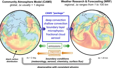
1" Community Atmosphere Model (CAM5)
global, Δx usually > 1 degree
black carbon distribution
Weather Research & Forecasting (WRF) regional, Δx ranges from 1 to 100 km
downscaling with consistent physics boundary conditions (meteorology, aerosol, chemistry, surface flux)
improved treatments
dx = 2 deg dx = 20 km
CAM5%“package”%
deep"convec*on" shallow"convec*on"
boundary"layer" microphysics" frac*onal"cloud"
aerosol"
emissions"
Fig. 1. Schematic diagram of the downscaling modeling framework with consistent physics between CAM5 and WRF.
the parameterizations developed by the global and regional modeling communities.
2 Model implementation
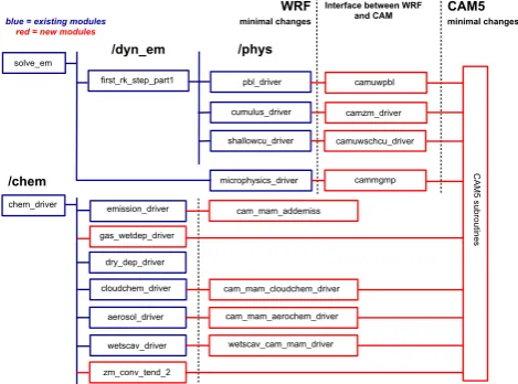
Most of the physics parameterizations from CAM5 (Neale et al., 2010) were transferred to WRF. The suite of parame-terizations illustrated in Fig. 1 is introduced through “inter-face routines” that connect the parent model infrastructure to each parameterization. These interface routines serve the purpose of converting the model state and other variables into the form expected by each parameterization. They de-termine the shape of arrays to send into the parameteriza-tion such as individual columns or 3-dimensional volumes, flip the vertical ordering of arrays, calculate derived vari-ables such as alternate ways of viewing humidity, etc. Both community models employ interface routines, but they are structured differently. Minor modifications to some param-eterizations were unavoidable because of differences in the code infrastructure and model design, and occasionally be-cause some fields were already available in WRF so re-dundant variants were removed (details are provided be-low). Figure 2 illustrates how the CAM5 physics modules were implemented in WRF. These modules were released in April 2013 as part of WRF (and WRF-Chem) version 3.5, and can be downloaded from the WRF model users web-site at http://www.mmm.ucar.edu/wrf/users/. The configura-tion of WRF-Chem running with the CAM5 physics suite has passed a regression test that the model produces the ex-act same results when using different number of processors.
blue = existing modules red = new modules
Interface between WRF
and CAM minimal changes minimal changes /phys camzm_driver camuwpbl camuwschcu_driver C AM5 su bro uti ne s cammgmp /dyn_em
WRF CAM5
solve_em first_rk_step_part1 cumulus_driver pbl_driver shallowcu_driver microphysics_driver /chem
chem_driver emission_driver cam_mam_addemiss
gas_wetdep_driver
zm_conv_tend_2
wetscav_driver wetscav_cam_mam_driver aerosol_driver cam_mam_aerochem_driver cloudchem_driver cam_mam_cloudchem_driver
dry_dep_driver
Fig. 2. Partial flow chart of the code implementation of the CAM5 physics suite within the WRF model, where blue denotes exist-ing WRF modules and red denotes modules associated with CAM5 physics and their interfaces with WRF.
(Zhang and Mcfarlane, 1995) with modifications to use a di-lute plume to calculate convection depth and CAPE (Neale et al., 2008) and convective momentum transport (Richter and Rasch, 2008), (4) the two-moment cloud microphysics scheme (Gettelman et al., 2008; Morrison and Gettelman, 2008), and (5) the three-mode (Aitken, accumulation, and coarse) version of the Modal Aerosol Module (MAM3) (Liu et al., 2012) that simulates black carbon, mineral dust, sea salt, sulfate, secondary organic aerosols, and primary or-ganic matter. The aerosol direct and indirect effects from CAM5 are also replicated in Chem. MAM3 in WRF-Chem is coupled with a modified version of carbon-bond mechanism (CBM) gas-phase chemical mechanism called “CBMZ” (Zaveri and Peters, 1999). In contrast, trace gas chemistry in standard CAM5 is simulated with a simple treat-ment that treats oxidation of sulfur dioxide and dimethyl sulfide as well as production and loss of hydrogen perox-ide using climatological values of ozone, and hydroxyl, hy-droperoxyl, and nitrate radicals (Neale et al., 2010) from a previously performed Model for OZone and Related Tracers (MOZART) (Emmons et al., 2010) simulation.
CAM5 includes a cloud macrophysics scheme (Park et al., 2014) that treats fractional cloudiness and condensa-tion/evaporation rates within stratiform clouds. The cloud parameterization in WRF typically does not account for fractional clouds, even when used at coarse resolutions that would benefit from such a treatment. The condensa-tion/evaporation rates in WRF are determined by assuming an instantaneous adjustment to saturation. The CAM5 pa-rameterization uses a rather complex treatment of fields pro-duced by other model components in its treatment of these processes. Because the time discretization and the order of parameterization and atmospheric dynamic updates are quite
different between CAM and WRF, porting the CAM5 macro-physics parameterization to WRF is quite difficult. Hence, we implemented a simplified module for the treatment of cloud macrophysics. For stratiform clouds, we implemented the subgrid-scale cloud fraction, condensation, and evapo-ration using the same triangular probability density func-tion (PDF) formulafunc-tion as the CAM5 cloud macrophysics scheme. Tunable parameters were set to standard CAM5 val-ues for a 2-degree grid spacing: threshold relative humidity of 88.75 % for low clouds (reduced to 78.75 % for low clouds over land without snow), 80 % for high clouds, and inter-polated thresholds for the mid-level clouds. The parameter-ization produces condensation and evaporation for subgrid clouds with changing cloud fraction (Park et al., 2014; Rasch and Kristjansson, 1998), even if the cell is sub-saturated. The deep and shallow convective cloud fractions are diagnosed from deep and shallow convective mass fluxes, respectively. The treatment of convective detrainment of liquid and ice cloud condensates (both mass and number) follows CAM5, but the detrainment rates in WRF are applied after the con-vection scheme is called instead of in a separate macro-physics module. When the CAM5 micromacro-physics scheme is selected, the total cloud fraction (the combination of strati-form as well as deep and shallow convective cloud fraction) is computed and used in the radiative transfer calculation by overwriting the standard WRF cloud fraction values calcu-lated in the radiative transfer interface routine (Hong et al., 1998). This simpler macrophysics parameterization produces clouds that are very similar to CAM5, but the implementa-tion was much easier, and it requires minimal code modifi-cations to switch between allowing a continuous cloud frac-tion (as in CAM5) and binary cloud fracfrac-tion (as in the tradi-tional WRF) to explore the consequences of the treatment of subgrid clouds (Gustafson Jr. et al., 2013). Changes in cloud fraction between two time steps also result in activation of in-terstitial aerosol or resuspension of cloud-borne aerosol, re-spectively (Abdul-Razzak and Ghan, 2000; Liu et al., 2012; Ovtchinnikov and Ghan, 2005), when running WRF-Chem with the MAM3 option.
very small time steps (e.g., 1 min or less) compared to CAM5 (30 min).
We have embedded the MAM3 as one option of the WRF-Chem, and aerosol processes and their interactions with ra-diation and clouds follow CAM5 formulations (Ghan et al., 2012; Liu et al., 2012) with a few minor modifications. A slightly different version of the Rapid Radiative Transfer Model for general circulation models (RRTMG) (Iacono et al., 2008; Mlawer et al., 1997) is used, and the existing aerosol optical property module in WRF-Chem (Barnard et al., 2010; Fast et al., 2006), which follows the same method-ology and assumptions as CAM5, is employed. Differences between the CAM5 and WRF-Chem aerosol optics codes are negligible, since the formulation and the mixing assumptions (for refractive indices) of the two models are essentially the same. Our package also supports a “prescribed aerosol” op-tion for the cloud microphysics that can be used for con-figurations of WRF and for WRF-Chem simulations when aerosol–cloud interactions are disabled. In this configuration, the cloud parameterization uses prescribed aerosol numbers and masses for cloud droplet nucleation, with the aerosol mass derived from the prescribed aerosol number and size distribution of each mode.
Multiple aerosol surface deposition velocity calculations are available in WRF-Chem when running with MAM3, and the CAM5 formulation that includes sedimentation, turbu-lent settling, and molecular adhesivity at the lowest model layer (Zhang et al., 2001) is one available option. However, CAM5 also calculates sedimentation velocities above the lowest model layer, but this is not treated in WRF-Chem. The omission of this process is expected to have very little effect on the life cycle of fine particles (i.e., aerosols in the Aitken and accumulation modes), but may have some effect on the life cycle of the largest particles (i.e., coarse-mode aerosols). The full effect of including sedimentation of aerosols in an RCM requires further investigation.
The MAM aerosol package distinguishes between intersti-tial and borne aerosols. In CAM5, advection of cloud-borne aerosols is neglected (Ghan and Easter, 2006). This may produce some error at higher resolution, so we advect both interstitial and cloud-borne aerosols in WRF-Chem.
The convective relaxation timescale (τ )in the deep con-vection scheme is usually set to be 3600 s in CAM5. With increasing spatial resolution, the model dynamics can pro-duce CAPE at a rate that cannot be removed by the convec-tion with a largeτ, producing fallacious “grid-scale storms” (Williamson, 2013). To address this issue, we have intro-duced a simple formula in WRF version 3.5 to determineτ
as a function of grid spacing with a lower bound of 600 s:
τ=max
τmin, τmax·
1x
1xref
,
whereτminis 600 s,τmaxis 3600 s,1x is the grid spacing,
and 1xref is the reference grid spacing, set to be 275 km
corresponding to the 2.5 degree grid-spacing in the tropics.
Nonetheless, in this study, we deliberately keep all tunable parameters, includingτ, at the same values as used in CAM5 (e.g.,τ =3600 s) for the purpose of exploring the resolution dependence of the parameterizations.
3 From CAM5 to WRF-Chem: the dynamical
downscaling procedure
We have developed a dynamical downscaling procedure for this study that (1) minimizes inconsistencies between the pa-rameterizations in the global model CAM5 and the regional model WRF-Chem, (2) facilitates a comparison of simula-tions between CAM5 and WRF-Chem with CAM5 physic, and (3) produces simulations that agree closely with ob-served meteorological events. We run CAM5 at a low cli-mate model resolution of 1.9 by 2.5 degree (nominally, “2-degree”) grid spacing with 56 levels in the vertical as an “offline model” (Lamarque et al., 2012; Ma et al., 2013b; Rasch et al., 1997), where the model’s winds, temperature, and pressure fields are constrained to agree with time in-terpolated fields from the ERA-Interim reanalysis (Dee et al., 2011), and there is a “wind-mass adjustment” made to the wind fields to make them consistent with the time evo-lution of the surface pressure field. The offline methodol-ogy has been routinely used for studying the atmospheric tracer transport problems (e.g., Ginoux et al., 2001; Jacob et al., 1997; Lawrence et al., 1999; Liu et al., 2009; Ma et al., 2013a). In the offline CAM5 configuration, water sub-stances and aerosols are allowed to evolve freely according to the CAM5 parameterization suite. The model simulation is archived at 6 h intervals. Meteorological fields (winds, perature, pressure, and humidity), surface fields (winds, tem-perature, pressure, latent and sensible heat flux, sea surface temperature, and snow height), and tracers (aerosols, trace gases, water vapor, and liquid and ice cloud condensates) are extracted from the archive and used as the initial and bound-ary conditions for the WRF-Chem simulations. A MOZART simulation is used to provide the initial and boundary condi-tions for the additional trace gas species in CBMZ. In these simulations, surface latent and sensible heat fluxes from the CAM5 simulation are used to avoid a resolution dependence of the moisture and heat sources, although they could also be calculated within WRF from its surface layer scheme cou-pled with a land model such as the Community Land Model of the CESM, which is embedded in WRF version 3.5. For the same reason, the effect of topography due to different res-olutions is also removed in this study by replacing the stan-dard WRF-Chem topography with the 2-degree CAM5 to-pography. The vertical sigma coordinate used in WRF is con-figured to match the sigma-pressure hybrid coordinate used in CAM5 at the initial time step, which has 45 levels from the surface to 20 hPa.
Measurements and Models, of Climate, Chemistry, Aerosols, and Transport (POLARCAT) Model Intercomparison Project (POLMIP). This inventory was compiled by Louisa Em-mons and is available for download at ftp://acd.ucar.edu/ user/emmons/EMISSIONS/arctas_streets_finn/. It contains anthropogenic emissions from David Streets’ inventory for Arctic Research of the Composition of the Troposphere from Aircraft and Satellites (ARCTAS) (Jacob et al., 2010), bio-genic emissions (Granier et al., 2011), and aerosol emis-sions from fires (Wiedinmyer et al., 2011). However, it does not include some recently identified aerosol sources such as gas flaring and domestic emissions over the Arc-tic that might result in underprediction of aerosol concen-tration in the Arctic (Stohl et al., 2013). The POLMIP emis-sion inventory includes mass emisemis-sions of primary aerosols, aerosol precursor gases, and other trace gases that are used by CBMZ. The emission data processing follows Liu et al. (2012). A small fraction (2.5 %) of the sulfur sources are emitted as primary sulfate. Anthropogenic sulfate emis-sions are partitioned 85 %/15 % between the accumulation and Aitken mode, and volcanic sulfate emissions are parti-tioned 50 %/50 % in those modes. Secondary organic aerosol emissions are produced using fixed yields from isoprene, terpene, toluene, and higher molecular weight alkanes and alkenes precursors. Black carbon, primary organic matter, sulfate, and sulfur emissions from fires are vertically dis-tributed in accordance with the spatially and temporally var-ied vertical profiles described in the AEROsol model in-terCOMparison project (AeroCom) (Dentener et al., 2006; Textor et al., 2006). Aerosol number emissions are calcu-lated from mass emissions using the assumed sizes listed in Liu et al. (2012). Emissions of aerosols and trace gases were first apportioned to the CAM5 grid and then regridded to all WRF-Chem grids, so all emissions have the same spatial de-tail. The MAM3 sea salt and dust emissions are computed online in CAM5 as a function of surface wind speed, and similar parameterizations exist in WRF-Chem as well. How-ever, for the purpose of this paper, we prescribe sea salt and dust emissions in the WRF-Chem with the 6-hourly instanta-neous emissions from the CAM5 simulation to eliminate the effect of resolution dependency of these aerosol sources.
4 The aerosol model test-bed case
There have been numerous field campaigns in different re-gions of the world that could be used to evaluate the per-formance of the CAM5 physics modules within the regional WRF model framework. We first focus on the high-latitudes because it is a vulnerable region for climate change (e.g., Screen and Simmonds, 2010; Serreze et al., 2009), and there are still large uncertainties regarding the role of aerosols in the Arctic (north of 66.5◦N) with documented deficien-cies in aerosol transport into the Arctic simulated by GCMs (Lee et al., 2013; Textor et al., 2006; Wang et al., 2013).
To better understand the factors controlling changes in at-mospheric composition and climate over the Arctic, several field campaigns were conducted in the vicinity of Alaska dur-ing the Arctic haze season (Law and Stohl, 2007; Quinn et al., 2007) in April 2008 as part of the International Polar Year. Three campaigns were conducted, including ARCTAS (Jacob et al., 2010) supported by National Aeronautics and Space Administration (NASA), the Aerosol, Radiation, and Cloud Processes affecting Arctic Climate (ARCPAC) cam-paign (Brock et al., 2011) supported by National Oceanic and Atmospheric Administration (NOAA), the Indirect and Semi-Direct Aerosol Campaign (ISDAC) (McFarquhar et al., 2011) supported by Department of Energy (DOE), and Euro-pean campaigns within the POLARCAT project.
An overview of the meteorological conditions observed during the spring of 2008 is described by Fuelberg et al. (2010) and the observed aerosol properties are docu-mented in de Villiers et al. (2010). The ATR-42 (France), Convair-580 (Canada), DC-8 (NASA), G-1 (DOE), P-3B (NASA), and the WP-3D (NOAA) research aircraft sam-pled meteorological, trace gases, and aerosol quantities us-ing various instruments. Two remote sensus-ing instruments were also deployed: high spectral resolution lidar (HSRL) on the NASA B-200 aircraft that obtained profiles of aerosol backscatter, extinction, and depolarization, and the differen-tial absorption lidar (DIAL) on the DC-8 aircraft that ob-tained profiles of ozone and aerosol backscatter. Most of the aircraft for ARCTAS, ARCPAC, and ISDAC flew over and in the vicinity of Alaska, and a few DC-8 and WP-3D tran-sects were made over the North Pole and between Alaska and Greenland, while the ATR-42 sampled air masses over northern Scandinavia. In addition to aircraft sampling, rou-tine surface measurements were collected at Barrow, Alaska (71.32◦N, 156.62◦W), from NOAA’s long-term climate re-search station and DOE’s Atmospheric Radiation and Mea-surement (ARM) climate research facility.
2011; Spackman et al., 2010). Cloud liquid water content and ice water content measured by Convair-580 (Jackson et al., 2012) are used to evaluate the model simulations of clouds.
In addition to the aircraft measurements, we also use other observational data to evaluate the model simulations. For aerosols, we use the surface BC measurements from a par-ticle soot absorption photometer (PSAP) at Barrow, Alaska, and the aerosol optical thickness (AOT) measurements from Aerosol Robotic NETwork (AERONET) (Holben et al., 1998) at Barrow and Bonanza Creek, Alaska. Measurements at the DOE’s ARM North Slope of Alaska (NSA) site at Bar-row, Alaska, are used to evaluate the simulated clouds. The Liu and Illingworth (2000) retrieval is used to evaluate the ice water content (IWC), and the Liao and Sassen (1994) data product is used to evaluate the liquid water content (LWC). For the column integrated ice water path (IWP) and liquid water path (LWP), we use the ARM Best Estimate (ARMBE) data products (Xie et al., 2010) while acknowledging the fact that multiple retrievals show 20–30 % (for LWP) and 10– 60 % (for IWP) uncertainty (Zhao et al., 2012). The ARMBE data product is also used to evaluate the total column precip-itable water. To assess the fidelity of the simulated precipita-tion, we used the 1-degree Global Precipitation Climatology Project (GPCP) daily precipitation data product.
5 Resolution dependence of long-range transport of
aerosols and aerosol–cloud interactions
Aerosol–cloud interactions remain one of the largest uncer-tainties in climate projections. These interactions occur at subgrid scales in most atmospheric models except for large eddy simulations. Deficiencies in the description of these in-teractions are believed to lead to high estimates of aerosol indirect forcing (Wang et al., 2012) and the underestimation of aerosol concentrations in remote regions such as the Arc-tic (Koch et al., 2009; Lee et al., 2013; Rasch et al., 2000; Shindell et al., 2008; Textor et al., 2006; Wang et al., 2013). The aerosol indirect forcing can also be amplified due to data aggregation from grid-box averages (McComiskey and Feingold, 2012). Increasing model resolution to reduce the subgrid inhomogeneity and to better resolve aerosol plumes (Weigum et al., 2012) may reduce this model bias. In this section, we document the resolution dependence of aerosol concentration and aerosol–cloud interactions in a high lati-tude region.
The offline CAM5 simulation was started on 1 Jan-uary 2008. Water vapor, condensate, and aerosol fields were allowed to spin up for 3 months, and simulation results from 1 April to 1 May 2008 were analyzed and used for initial and boundary conditions for regional downscaling model-ing. The regional modeling domain encompasses northeast-ern Asia, the northnortheast-ern Pacific Ocean, and northwestnortheast-ern North America (Fig. 1, right panel) so that the primary aerosol transport pathway from Asia to Alaska (Ma et al., 2013a, b)
is included. For all our WRF-Chem simulations, the winds and temperature were nudged towards the offline CAM5 fields (which comes from the ERA-Interim reanalysis) us-ing a timescale of 1 hour to constrain those fields to be close to the large-scale analyzed fields since our focus was the life cycle of aerosols and clouds. Simulations were per-formed using horizontal grid spacings of 160, 80, 40, 20, and 10 km (labeled as WRF_160 km, WRF_80 km, WRF_40 km, WRF_20 km, and WRF_10 km, respectively) to explore the behavior of the cloud and aerosol parameterizations as a function of grid spacing. Note that since the lowest resolu-tion of WRF-Chem used in this study (160 km) is still finer than the CAM5 grid (1.9 by 2.5 degrees) in the mid-latitudes where most aerosol emissions and wet scavenging take place, there might be differences between these two model simu-lations. In addition, the differences in dynamical cores and time steps between the two models might also contribute to different results.
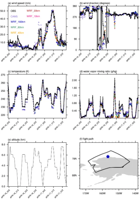
Fig. 3. The simulated and observed (a) wind speed (m s−1), (b) wind direction (degree), (c) temperature (K), and (d) water
va-por mixing ratio (g kg−1)at (e) altitude along (f) the DC-8 flight
path on 16 April 2008, during the ARCTAS field campaign. The
blue star in (f) denotes the location of Barrow, Alaska (71.32◦N,
156.62◦W).
for convective clouds is found to decrease slightly with in-creasing resolution, from 20.7 % for the 160 km simulation to 17.6 % for the 10 km simulation, contributing 4.1 % and 2.6 % of the total cloud fraction, respectively. While CAM5 and WRF_160 km produce similar features, the remaining differences between these two simulations can be attributed to the differences in their resolutions, time steps, and dynam-ical cores. We have performed a sensitivity test (not shown) and found that the difference in the simulated clouds and aerosols between these two model simulations can be greatly reduced by setting the CAM5 time step (30 min) to a smaller time step (5 min) that is closer to WRF’s time step (1 min). The model dependence on time step is currently under inves-tigation and will be documented in a separate paper.
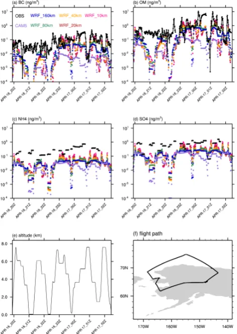
As previously mentioned, global models have difficulties simulating aerosols in the Arctic, producing a significant low bias of aerosol concentrations especially near the surface (Shindell et al., 2008). Using the same aircraft transect in Fig. 3, we show that aerosol mass concentrations of black
Fig. 4. Time series of observed and simulated (a) liquid water
con-tent (g m−3)and (b) ice water content (g m−3)and 5th, 25th, 50th,
75th, and 95th percentile of observed and simulated (c) liquid
wa-ter content (g m−3)and (d) ice water content (g m−3)over all of
the aircraft flights. (e) and (f) depict the altitude and flight path, re-spectively, of 15 Convair-580 flight paths during the ISDAC field campaign. Vertical bars in (a) and (b) show the range of the 5th and 95th percentile of the observations within each hour.
carbon, organic matter, ammonia, and sulfate are low in all model simulations by about 1 order of magnitude (Fig. 5). Model simulations also exhibit occasional drops in aerosol concentrations when the aircraft measurements are near the surface, showing 2–3 orders of magnitude lower aerosol con-centrations than observations. Increasing resolution reduces the bias, but even with the smallest grid spacing of 10 km a significant bias remains. Since these aircraft measurements were taken a few days before an episode with much higher aerosol concentrations that started around 20 April, this re-sult suggests that the model has a much lower background aerosol concentration. Meanwhile, the variability of the sim-ulated aerosols increases with resolution because the spa-tially inhomogeneous distribution of aerosols is better re-solved in high-resolution simulations.
Fig. 5. The observed and simulated concentrations (ng m−3)of (a) black carbon, (b) organic matter, (c) ammonium, and (d) sulfate at (e) altitude along (f) the DC-8 flight path on 16 April 2008, during the ARCTAS field campaign.
taken between 6 and 17 April. This period is representa-tive of the background aerosol state, as opposed to the high aerosol concentrations associated with transport of anthro-pogenic and biomass burning plumes over Alaska around 20 April. All model simulations are about 2–3 orders of magnitude too low at the surface, and about 1–2 orders of magnitude too low aloft. In general, the higher resolution model simulations show greater variability of BC concentra-tion that results from narrower aerosol plumes with higher concentrations. The concentrations outside of the plume’s centers are also lower since the low-resolution simulations tend to dilute the aerosols over a larger region. Decreasing grid spacing from the 160 to 10 km grid spacing reduces the low bias of BC at the surface by about a factor of 5. Figure 7 compares simulated surface BC concentrations at Barrow with PSAP measurements of equivalent BC (EBC) (Sharma et al., 2006) at the surface with the specific atten-uation of 10 m2g−1 (S. Sharma, personal communication, 2012). The monthly mean EBC concentration is about 2–3 orders of magnitude higher than model simulations (Fig. 7a),
Fig. 6. Vertical profile of the observed and simulated median, 5th
and 95th percentile black carbon concentration (ng m−3), sampled
from a total of eight P3B and DC-8 flights on 6–17 April 2008, during the ARCTAS field campaign.
and the models consistently underpredict the background surface BC concentration by about 3–5 orders of magnitude, and by about 1–3 orders of magnitude when the episode of high BC concentration starts around 20 April when the ob-served BC increases from about 70 ng m−3 to 500 ng m−3,
and the model simulations also increase from about 0.1 to 50 ng m−3(Fig. 7b). This model bias reduces monotonically
with increasing resolution. These results show that the high-resolution simulations are able to deliver BC from the source regions over Asia to Barrow when the high BC concentra-tion episode took place, even though all resoluconcentra-tions fail to produce the background BC concentration at the observed level. The low background BC might be attributed to either model deficiencies in transporting aerosols into the Arctic due to weaker eddy transport (Ma et al., 2013b) and stronger wet scavenging in the mid-latitudes (Wang et al., 2013), the underestimation or omission of aerosol sources (Stohl et al., 2013; Q. Wang et al., 2011), or a combination of both. The uncertainty associated with the emission inventory is con-sidered to be a factor of 2 or more (Bond et al., 2004; Ra-manathan and Carmichael, 2008), and its effect on the simu-lation requires further investigations.
Fig. 7. Surface black carbon concentration (ng m−3)over Barrow from model simulations and PSAP measurements: (a) monthly av-erage and (b) time series.
magnitude with resolution, from 3.7 ng kg−1for the 160 km grid-spacing simulation to 51.6 ng kg−1for the 10 km grid-spacing simulation (Fig. 8h and l). The BC concentrations over Barrow in the high-resolution simulations averaged over the corresponding 160 km grid cell increase monoton-ically with increasing resolution, reaching 50.9 ng kg−1 in
the 10 km grid-spacing simulation. The instantaneous max-imum BC concentration within the corresponding 160 km grid cell over Barrow increases by about a factor of 30 (from 3.7 ng kg−1to 95.6 ng kg−1), suggesting that the spa-tial variability of BC also increases with resolution, consis-tent with previous studies (Gustafson Jr. et al., 2011; Qian et al., 2010). These results suggest that the unrealistic assump-tion of homogeneous aerosol distribuassump-tion within each grid cell in CAM5 might be at least partly responsible for the un-derestimation of aerosol transport into the Arctic, and some of the bias that remains in the high-resolution simulations is likely due to the low values of BC present in the boundary conditions for the regional simulations delivered to the re-gion by the low-resolution CAM simulations.
Figure 8g–l show that the large difference in surface BC concentration at Barrow is related to the filamentary structure of aerosol plumes, which can only be resolved in the high-resolution simulations, and the transport of BC from north-east Asia to Barrow is sensitive to this flow feature. In high-resolution simulations, a concentrated aerosol plume located in the gap between the clouds of two frontal systems is evi-dent (Fig. 8f and l). Since clouds and the associated precip-itation play a critical role removing aerosols in CAM5 (Liu et al., 2012; Wang et al., 2013) and the poleward transport
Fig. 8. The simulated (a)–(f) cloud fraction and (g)–(l) black carbon
mixing ratio (ng kg−1)at the second lowest model layer at 00Z of
20 April 2008. Numbers in (a)–(f) are the domain average cloud fraction. In (g)–(l), black carbon mixing ratios at the second lowest model over Barrow are given, and numbers in parentheses are the maximum black carbon concentration within the 160 km cell over Barrow.
of aerosols in these latitudes depends on features driven by these eddies (Ma et al., 2013b), this cloudless transport path-way between two mesoscale eddies facilitates the transport of aerosols into the Arctic. In low-resolution simulations, the coarse grids are unable to resolve these filamentary features associated with mesoscale eddies; hence, aerosols are subject to wet removal within clouds along the path.
Fig. 9. Time series of total column burden of (a) black carbon, (b) mineral dust, (c) sea salt, (d) sulfate, (e) secondary organic aerosol,
and (f) primary organic matter (106kg m−2)in the Arctic (north of
66.5◦N).
over ocean. Another possible explanation is that the sea salt aerosols have a source that is not remote in the regional sim-ulations, so it is not dependent on the boundary conditions. Although sea salt emission would generally be sensitive to surface wind speeds, and thus could have a resolution depen-dence (higher wind speeds being resolved with smaller grid spacings), this effect is not present in our simulation because the sea salt emissions have been prescribed from CAM5 for all the WRF-Chem simulations.
As aerosol and cloud distributions and loadings evolve, the aerosol–cloud interactions may change accordingly. One convenient means of characterizing the relationship between aerosols and clouds is “cloud susceptibility to aerosols”, de-fined as the fractional increase of cloud LWP to fractional increase of AOT (e.g., Quaas et al., 2009; M. Wang et al., 2011), often expressed as the slope of a measure of frac-tional change in a cloud property related to its radiative effect (in this case using liquid water column burden) to fractional change in aerosol amount (in this case using the AOT). CAM5 has a very high value of susceptibility (Wang et al., 2012), and part of this behavior can be attributed to parametric uncertainty (Liu et al., 2014). Figure 10 dis-plays the susceptibility, calculated from hourly model output of AOT and LWP for the whole simulation period at every grid point over the entire domain (excluding the buffer zone of the lateral boundary), as a function of horizontal resolu-tion. The cloud susceptibility to aerosols decreases by about 45 % in the highest-resolution simulation. The WRF_10 km
Fig. 10. Cloud susceptibility to aerosol forcing as a function of model horizontal grid spacing.
simulation shows much lower cloud susceptibility, which leads to weaker scavenging and results in larger aerosol bur-dens and higher long-range transport of aerosols as shown in Fig. 9. The reduction of cloud susceptibility with increasing resolution can be largely explained by the fact that aerosol plumes and clouds are less collocated in high-resolution sim-ulations as shown in Fig. 8. Clouds and precipitation occur in narrower spatial regions, and the occurrence of clouds and precipitation in any given model column is less fre-quent in many columns, producing weaker aerosol–cloud in-teractions. Other physical mechanisms may also be sensitive to resolution (e.g., autoconversion and accretion) and affect cloud susceptibility and aerosol indirect forcing. These is-sues are being explored and will form the basis of a later study.
6 Comparison of the CAM5 physics with a common
WRF parameterization suite
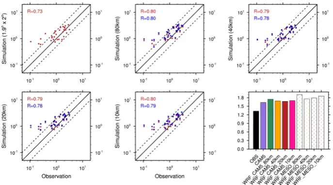
Fig. 11. Scatterplots of aerosol optical thickness from model simulations that utilize the CAM5 (red) and WRF (blue) physics suite, evaluated
against AERONET observations at Barrow (71.31◦N, 156.67◦W) and Bonanza Creek (64.74◦N, 148.32◦W).
significantly different, and provide an opportunity to quan-tify the performance of alternative process modules before they are incorporated and used by global climate models. Such a comparison could be expanded to provide insights into the model’s structural uncertainty (deficiencies associ-ated with specific treatments of various physical and chem-ical processes in the model parameterizations) and help to identify the components that produce the largest differences in simulations by changing process representations one at a time. For brevity, we restrict our analysis to a demonstration of capability rather than quantifying effects of each process in the two different parameterization suites.
The WRF_MESO configuration includes a double mo-ment cloud microphysics scheme (Morrison et al., 2009), the Grell and Devenyi (2002) cumulus ensemble param-eterization, an operational boundary layer scheme for the Eta model (Janjic, 2002) that employs a turbulent kinetic energy formulation (Mellor and Yamada, 1982), the Noah land surface model (Chen and Dudhia, 2001), and the 8-size bin version of Model for Simulating Aerosol Interactions and Chemistry (MOSAIC) aerosol model (Zaveri et al., 2008). The WRF_MESO configuration does not treat aerosol wet removal and vertical transport by subgrid convective clouds, but does represent wet removal when the cell-averaged values indicate clouds are present, and aerosols undergo vertical transport by resolved winds and turbulent processes. Our analysis later in this section shows that these differences do not contribute to large differences in the simulations over this high-latitude domain. Both model configurations are run at multiple grid spacings: 80, 40, 20, and 10 km (labeled as “WRF_CAM5_80 km”, “WRF_ CAM5_40 km”, “WRF_CAM5_20 km”, “WRF_ CAM5_10 km”, “WRF_MESO_80 km”, “WRF_MESO_ 40 km”, “WRF_MESO_20 km”, and “WRF_MESO_
10 km”). We performed the evaluation within a smaller domain that encompasses Alaska and its vicinity (area enclosed by purple lines in Fig. 12f), approximately 3000 km by 3000 km in total area. All WRF simulations use the global CAM5 results for the initial and boundary conditions for model state (meteorology, cloud condensate, aerosols, and trace gases). The same emission inventory is used to drive all model simulations. The MAM3 aerosol concentrations and emissions from CAM5 are mapped to the corresponding MOSAIC aerosol species in the emission interface subroutine as well as the initial and boundary conditions of WRF_MESO simulations. While the WRF-Chem model with the CAM5 physics suite uses prescribed sea salt and dust emissions as well as surface moisture and heat fluxes archived from the offline CAM5 simulation, the WRF_MESO simulations compute these fields as a function of surface wind speed.
Figure 11 shows that when driven by the same initial and boundary conditions from the CAM5 simulation, all the WRF_CAM5 and WRF_MESO simulations underpredict AOT by 1 order of magnitude compared to AERONET obser-vations at Barrow and Bonanza Creek. Increasing resolution only has a very modest improvement, and the WRF_CAM5 and WRF_MESO simulations produce similar results. Ver-tical profiles are also similar between model configurations, and all simulations are biased low by 1 order of magnitude near the surface compared with the observations calculated from the samples obtained from the ARCPAC field campaign (Fig. 12, and see Koch et al., 2009, for details on data pro-cessing).
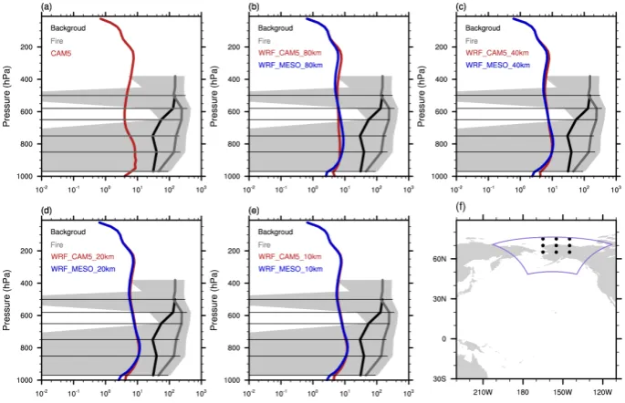
Fig. 12. Monthly mean vertical profiles of BC mixing ratio (ng kg−1)from model simulations that uses the CAM5 (red) or WRF (blue) physics suite, compared with observations from the ARCPAC field campaign (dotted area). The purple line encloses the area of the WRF domain.
most aerosols in the Arctic originate from remote sources (Ma et al., 2013a) and enter this WRF domain through the lateral boundary conditions. Since aerosol concentrations in the coarse-resolution CAM5 simulation are significantly un-derestimated (Ma et al., 2013b; Wang et al., 2013) due to a combination of strong wet scavenging over the ocean and weaker eddy transport in the low-resolution CAM5 simu-lation, and underestimation of emissions of aerosols and their precursors, the regional WRF simulations receives low aerosol inflows from the model’s western boundary over Bering Sea and southern boundary over the Pacific Ocean, leading to a low bias for aerosol concentrations and AOT. In addition, since the aerosol plumes reaching this region are already aged, different treatments of aerosol chemistry between MAM3 and MOSAIC have only marginal effects on the simulation. For regional domains containing a major source region where local emissions dominate and aerosols are less aged, differences between MAM3 and MOSAIC can lead to significantly different aerosol simulations (not shown).
In spite of the strong influence from the lateral boundaries, there is still one noticeable difference between WRF_CAM5 and WRF_MESO: BC concentration near the surface is about a factor of 2 higher in the WRF_CAM5 simulations (Fig. 12). One possible explanation contributing to this difference is that the CAM5 physics suite takes into account the resuspen-sion of aerosol particles from evaporated raindrops, which is omitted in the WRF_MESO physics suite. Note that both the WRF_CAM5 and the WRF_MESO physics suite consider the aerosol resuspension process in decaying clouds (when cloud droplets evaporate). Further investigation is needed to
understand all differences between the two parameterizations and their effects on the simulation, and this modeling frame-work can be useful for such process-level studies.
The simulated total column water vapor and precipitation rates in all model simulations are generally in good agree-ments with observations with high correlations and small bi-ases (Figs. 13 and 14). All model simulations overpredict precipitation when the observed precipitation is light but do much better for rain amounts above about 0.4 mm day−1. The correlation between model simulations and GPCP precipita-tion rate is very good for rain rates larger than 0.4 mm day−1 and poor below that. Increasing resolution generally has little effect on the daily precipitation in this high-latitude domain that is largely over land. However, resolution dependence is expected for instantaneous precipitation rates and precipita-tion over regions where synoptic and mesoscale features of moisture convergence are better resolved at higher resolu-tion.
Fig. 13. Scatterplots of total column precipitable water vapor (g m−2)from model simulations that utilize the CAM5 (red) and WRF (blue) physics suite evaluated against the ARM best estimates at Barrow.
Fig. 14. Scatterplots of the domain mean daily precipitation rate (mm day−1)from model simulations that utilize the CAM5 (red) and WRF
(blue) physics suite evaluated against the GPCP daily data averaged over the same domain.
et al. (2013) reached a similar conclusion that omitting the treatment of subgrid cloud in WRF running with CAM5 physics suite for typical mesoscale resolutions (grid spac-ing rangspac-ing from 4 to 32 km) results in a reduction of liq-uid and ice condensate amount. In addition, Fig. 15 also shows that the WRF_CAM5 simulations produce low liq-uid water condensate above 1.5 km compared with observa-tions, and the bias is improved with increasing resolution. In contrast, the WRF_MESO simulations do not show the same behavior. This model bias could be attributed to the model representation of ice cloud processes and rainwater treat-ment. For example, different rainwater treatment between the Morrison et al. (2009) scheme used in WRF_MESO simula-tions and the Morrison and Gettelman (2008) scheme used
in WRF_CAM5 simulations can produce different clouds because the emphasis of rain production can be shifted from autoconversion to accretion as the model changes its rainwater treatment from diagnostic rain (as used in the WRF_CAM5 cloud microphysics) to prognostic rain (as used in the WRF_MESO cloud microphysics), which re-duces the aerosol effect on clouds (Posselt and Lohmann, 2009). Quantification of the effect of each process in the two parameterizations is beyond the scope of this study and should be addressed by an independent study.
Fig. 15. Time series of vertical profiles of liquid water content (g kg−1)from ARM: (a) hourly mean, (b) hourly maximum, and (c) hourly
minimum, compared with the in-cloud liquid water content (g kg−1)from (d)–(g) WRF_CAM5 and (h)–(k) WRF_MESO simulations at
Barrow. Values of average liquid water content and frequency of occurrence of liquid cloud are given.
Fig. 16. Histograms (percentage) of (a) the observed liquid water path (g m−2)from ARM Cloud Retrieval Ensemble Dataset, and (b)–(i)
Fig. 17. Time series of vertical profiles of ice water content (g kg−1)from ARM: (a) hourly mean, (b) hourly maximum, and (c) hourly
minimum, compared with the in-cloud ice water content (g kg−1)from (d)–(g) WRF_CAM5 and (h)–(k) WRF_MESO simulations at
Barrow. Values of average ice water content and frequency of occurrence of ice cloud are given.
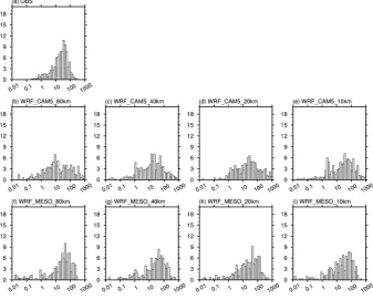
Fig. 18. Histograms (percentage) of (a) the observed ice water path (g m−2)from ARM Cloud Retrieval Ensemble Dataset, and (b)–(i) the
the WRF_MESO simulations in terms of both frequency of occurrence and monthly mean in-cloud ice water content. The in-cloud ice water path distributions between model simulations and observations are qualitatively similar, but the WRF_CAM5 simulations show more events of high ice water path, whereas the WRF_MESO simulations have more low ice water path events (Fig. 18). The distribu-tions of the frequency of occurrence for both ice and liq-uid clouds are found insensitive to model resolution. In addi-tion, the observations show a mean liquid-to-total water ra-tio of about 29.8 % in mixed phase clouds, higher than the WRF_CAM5 simulations (increasing from 13.4 % to 25.3 % with resolution) and lower than the WRF_MESO simulations (increasing from 40.4 % to 46.3 % with resolution). These differences highlight sensitivity to the different representa-tions of ice cloud processes between the two cloud micro-physics parameterizations. For example, while the Morrison et al. (2009) scheme treats the Wegener–Bergeron–Findeisen process explicitly by computing both the evaporation of liq-uid condensates and the deposition of water vapor in mixed phase clouds using cell-averaged quantities, the Morrison and Gettelman (2008) parameterization computes the deposi-tion rate by converting the subgrid in-cloud liquid to ice con-densates directly. This difference can lead to different ice de-position rates. Insights into the improvement on the ice cloud parameterization could be gained from further investigation. In summary, this modeling framework can be useful to probe effects of different parameterizations. We demon-strated that the CAM5 physics suite in WRF-Chem pro-duces a realistic regional meteorology and aerosol distribu-tions similar to simuladistribu-tions using a common set of the WRF parameterizations. Some improvements in the BC concen-tration near the surface, the frequency of occurrence of liq-uid water content, and the ice water condensate amount were produced by the CAM5 physics suite. However, the underes-timation of aerosols in the global model remains in the RCM. The low bias is insensitive to model resolutions and physics suites for this particular domain and the simulated period of time in this study, suggesting that much of the underestima-tion is caused by the low estimates of local emissions in this emission inventory and the low concentrations of BC enter-ing the region from the boundary condition values provided by CAM5.
7 Concluding remarks
The CAM5 physics parameterization suite has been recently ported to the WRF-Chem model. A downscaling modeling framework has been developed that minimizes inconsisten-cies between the global and regional models. This allows us to run the CAM5 physics suite over a range of scales. We use this downscaling modeling framework to evaluate the CAM5 physics at high resolution and to directly compare model pre-dictions with high-resolution field campaign data. The suite
was released as part of WRF (and WRF-Chem) version 3.5 in April 2013 for broader use by both the WRF and CAM com-munities for various research objectives. This manuscript de-scribes how the CAM5 parameterizations were implemented in WRF-Chem and provides an initial evaluation.
We ported the CAM5 physics suite in WRF using inter-face routines to minimize changes to the CAM5 codes (both formulation and programming). This approach (1) eases im-plementation of future updates, (2) minimizes the likelihood of changing the behavior of the parameterizations because of implementation issues, and (3) makes the CAM5 physics suite behave similarly in WRF and CAM when running at similar resolutions. Necessary minor modifications appear to have only marginal effects on the simulation. We extended the capabilities of WRF by adding parameterizations that are designed for larger space and timescales, and provided a means to compare simulations using different parameteri-zations within the same modeling framework to better assess the effects of different model treatments of aerosols, clouds, convections, and aerosol–cloud interactions. The new param-eterization suite supports a consistent treatment of subgrid-scale clouds, a feature that was previously neglected in WRF and WRF-Chem.
study focuses on only one case, and there are many parame-terization choices in WRF; other parameparame-terization combina-tions are likely to perform differently for this test-bed case as well as in other regions/seasons. Additional analyses and more case studies are needed to understand the overall per-formance of the CAM5 physics compared to other model treatments.
Acknowledgements. We thank our internal reviewer Minghuai Wang for his constructive comments on the manuscript. We thank Jennifer Comstock, Jiwen Fan, Andrew Gettelman, Sam-son Hagos, Anne JefferSam-son, Lai-Yung (Ruby) Leung, Kyo-Sun Lim, Greg McFarquhar, Hugh Morrison, John Ogren, Mikhail Ovchin-nikov, Sungsu Park, Yun Qian, Laura Riihimaki, Sangeeta Sharma, Hailong Wang, Kai Zhang, Yang Zhang, and Chun Zhao for helpful discussions and their advice with the model and various kinds of observational data. The surface observational data used in this study were obtained from the North Slope of Alaska site at Barrow, Alaska, a United States Department of Energy (DOE) Atmospheric Radiation Measurement Climate Research Facility. This work is primarily supported by the DOE’s Office of Science/Biological and Environmental Research, through Earth System Modeling Program (“Interactions of Aerosol, Clouds, and Precipitation in the Climate System” Science Focus Area). This work is also supported by a DOE Early Career grant awarded to William I. Gustafson Jr., and the Aerosol Climate Initiative within the Laboratory Directed Research and Development (LDRD) program at the Pacific North-west National Laboratory (PNNL). PNNL is operated for DOE by Battelle Memorial Institute under contract DE-AC06-76RLO 1830.
Edited by: R. Neale
References
Abdul-Razzak, H. and Ghan, S. J.: A parameterization of aerosol activation 2. Multiple aerosol types, J. Geophys. Res.-Atmos., 105, 6837–6844, doi:10.1029/1999jd901161, 2000.
Barnard, J. C., Fast, J. D., Paredes-Miranda, G., Arnott, W. P., and Laskin, A.: Technical Note: Evaluation of the WRF-Chem “Aerosol Chemical to Aerosol Optical Properties” Module using data from the MILAGRO campaign, Atmos. Chem. Phys., 10, 7325–7340, doi:10.5194/acp-10-7325-2010, 2010.
Bond, T. C., Streets, D. G., Yarber, K. F., Nelson, S. M., Woo, J. H., and Klimont, Z.: A technology-based global inventory of black and organic carbon emissions from combustion, J. Geophys. Res.-Atmos., 109, D14203, doi:10.1029/2003jd003697, 2004. Bretherton, C. S. and Park, S.: A New Moist Turbulence
Parame-terization in the Community Atmosphere Model, J. Climate, 22, 3422–3448, doi:10.1175/2008jcli2556.1, 2009.
Brock, C. A., Cozic, J., Bahreini, R., Froyd, K. D., Middlebrook, A. M., McComiskey, A., Brioude, J., Cooper, O. R., Stohl, A., Aikin, K. C., de Gouw, J. A., Fahey, D. W., Ferrare, R. A., Gao, R.-S., Gore, W., Holloway, J. S., HÜbler, G., Jefferson, A., Lack, D. A., Lance, S., Moore, R. H., Murphy, D. M., Nenes, A., Novelli, P. C., Nowak, J. B., Ogren, J. A., Peischl, J., Pierce, R. B., Pilewskie, P., Quinn, P. K., Ryerson, T. B., Schmidt, K. S., Schwarz, J. P., Sodemann, H., Spackman, J. R., Stark, H.,
Thomson, D. S., Thornberry, T., Veres, P., Watts, L. A., Warneke, C., and Wollny, A. G.: Characteristics, sources, and transport of aerosols measured in spring 2008 during the aerosol, radiation, and cloud processes affecting Arctic Climate (ARCPAC) Project, Atmos. Chem. Phys., 11, 2423–2453, doi:10.5194/acp-11-2423-2011, 2011.
Caya, D. and Biner, S.: Internal variability of RCM simulations over an annual cycle, Clim. Dynam., 22, 33–46, doi:10.1007/S00382-003-0360-2, 2004.
Chen, F. and Dudhia, J.: Coupling an advanced land surface-hydrology model with the Penn State-NCAR MM5 mod-eling system. Part I: Model implementation and sensitiv-ity, Mon. Weather Rev., 129, 569–585, doi:10.1175/1520-0493(2001)129<0569:Caalsh>2.0.Co;2, 2001.
Chou, C., Chiang, J. C. H., Lan, C. W., Chung, C. H., Liao, Y. C., and Lee, C. J.: Increase in the range between wet and dry season precipitation, Nat. Geosci., 6, 263–267, doi:10.1038/Ngeo1744, 2013.
Cubison, M. J., Ortega, A. M., Hayes, P. L., Farmer, D. K., Day, D., Lechner, M. J., Brune, W. H., Apel, E., Diskin, G. S., Fisher, J. A., Fuelberg, H. E., Hecobian, A., Knapp, D. J., Mikoviny, T., Riemer, D., Sachse, G. W., Sessions, W., Weber, R. J., Wein-heimer, A. J., Wisthaler, A., and Jimenez, J. L.: Effects of aging on organic aerosol from open biomass burning smoke in aircraft and laboratory studies, Atmos. Chem. Phys., 11, 12049–12064, doi:10.5194/acp-11-12049-2011, 2011.
Dee, D. P., Uppala, S. M., Simmons, A. J., Berrisford, P., Poli, P., Kobayashi, S., Andrae, U., Balmaseda, M. A., Balsamo, G., Bauer, P., Bechtold, P., Beljaars, A. C. M., van de Berg, L., Bid-lot, J., Bormann, N., Delsol, C., Dragani, R., Fuentes, M., Geer, A. J., Haimberger, L., Healy, S. B., Hersbach, H., Holm, E. V., Isaksen, L., Kallberg, P., Kohler, M., Matricardi, M., McNally, A. P., Monge-Sanz, B. M., Morcrette, J. J., Park, B. K., Peubey, C., de Rosnay, P., Tavolato, C., Thepaut, J. N., and Vitart, F.: The ERA-Interim reanalysis: configuration and performance of the data assimilation system, Q. J. Roy. Meteorol. Soc., 137, 553– 597, doi:10.1002/Qj.828, 2011.
Dentener, F., Kinne, S., Bond, T., Boucher, O., Cofala, J., Generoso, S., Ginoux, P., Gong, S., Hoelzemann, J. J., Ito, A., Marelli, L., Penner, J. E., Putaud, J.-P., Textor, C., Schulz, M., van der Werf, G. R., and Wilson, J.: Emissions of primary aerosol and precur-sor gases in the years 2000 and 1750 prescribed data-sets for Ae-roCom, Atmos. Chem. Phys., 6, 4321–4344, doi:10.5194/acp-6-4321-2006, 2006.
Deser, C., Phillips, A. S., Tomas, R. A., Okumura, Y. M., Alexan-der, M. A., Capotondi, A., Scott, J. D., Kwon, Y. O., and Ohba, M.: ENSO and Pacific Decadal Variability in the Community Climate System Model Version 4, J. Climate, 25, 2622–2651, doi:10.1175/Jcli-D-11-00301.1, 2012.
de Villiers, R. A., Ancellet, G., Pelon, J., Quennehen, B., Schwarzenboeck, A., Gayet, J. F., and Law, K. S.: Airborne mea-surements of aerosol optical properties related to early spring transport of mid-latitude sources into the Arctic, Atmos. Chem. Phys., 10, 5011–5030, doi:10.5194/acp-10-5011-2010, 2010. Emmons, L. K., Walters, S., Hess, P. G., Lamarque, J.-F., Pfister,
(MOZART-4), Geosci. Model Dev., 3, 43–67, doi:10.5194/gmd-3-43-2010, 2010.
Fan, J. W., Ghan, S., Ovchinnikov, M., Liu, X. H., Rasch, P. J., and Korolev, A.: Representation of Arctic mixed-phase clouds and the Wegener-Bergeron-Findeisen process in climate models: Per-spectives from a cloud-resolving study, J. Geophys. Res.-Atmos., 116, D00t07, doi:10.1029/2010jd015375, 2011.
Fast, J. D., Gustafson, W. I., Easter, R. C., Zaveri, R. A., Barnard, J. C., Chapman, E. G., Grell, G. A., and Peckham, S. E.: Evolution of ozone, particulates, and aerosol direct ra-diative forcing in the vicinity of Houston using a fully coupled meteorology-chemistry-aerosol model, J. Geophys. Res.-Atmos., 111, D21305, doi:10.1029/2005jd006721, 2006.
Fast, J. D., Gustafson, W. I., Chapman, E. G., Easter, R. C., Rishel, J. P., Zaveri, R. A., Grell, G. A., and Barth, M. C.: The Aerosol Modeling Testbed a Community Tool to Objectively Evaluate Aerosol Process Modules, B. Am. Meteorol. Soc., 92, 343–360, doi:10.1175/2010bams2868.1, 2011.
Fuelberg, H. E., Harrigan, D. L., and Sessions, W.: A meteoro-logical overview of the ARCTAS 2008 mission, Atmos. Chem. Phys., 10, 817–842, doi:10.5194/acp-10-817-2010, 2010. Ganguly, D., Rasch, P. J., Wang, H. L., and Yoon, J. H.:
Cli-mate response of the South Asian monsoon system to an-thropogenic aerosols, J. Geophys. Res.-Atmos., 117, D13209, doi:10.1029/2012jd017508, 2012a.
Ganguly, D., Rasch, P. J., Wang, H. L., and Yoon, J. H.: Fast and slow responses of the South Asian monsoon system to anthropogenic aerosols, Geophys. Res. Lett., 39, L18804, doi:10.1029/2012gl053043, 2012b.
Gent, P. R. and Danabasoglu, G.: Response to Increasing South-ern Hemisphere Winds in CCSM4, J. Climate, 24, 4992–4998, doi:10.1175/Jcli-D-10-05011.1, 2011.
Gettelman, A., Morrison, H., and Ghan, S. J.: A new two-moment bulk stratiform cloud microphysics scheme in the community atmosphere model, version 3 (CAM3). Part II: Single-column and global results, J. Climate, 21, 3660–3679, doi:10.1175/2008jcli2116.1, 2008.
Gettelman, A., Kay, J. E., and Shell, K. M.: The Evolution of Cli-mate Sensitivity and CliCli-mate Feedbacks in the Community At-mosphere Model, J. Climate, 25, 1453–1469, doi:10.1175/Jcli-D-11-00197.1, 2012.
Ghan, S. J. and Easter, R. C.: Impact of cloud-borne aerosol rep-resentation on aerosol direct and indirect effects, Atmos. Chem. Phys., 6, 4163–4174, doi:10.5194/acp-6-4163-2006, 2006. Ghan, S. J., Leung, L. R., Easter, R. C., and Abdul-Razzak,
K.: Prediction of cloud droplet number in a general circu-lation model, J. Geophys. Res.-Atmos., 102, 21777–21794, doi:10.1029/97jd01810, 1997.
Ghan, S. J., Leung, L. R., and McCaa, J.: A comparison of three different modeling strategies for evaluating cloud and radia-tion parameterizaradia-tions, Mon. Weather Rev., 127, 1967–1984, doi:10.1175/1520-0493(1999)127<1967:Acotdm>2.0.Co;2, 1999.
Ghan, S. J., Liu, X., Easter, R. C., Zaveri, R., Rasch, P. J., Yoon, J. H., and Eaton, B.: Toward a Minimal Representation of Aerosols in Climate Models: Comparative Decomposition of Aerosol Di-rect, SemidiDi-rect, and Indirect Radiative Forcing, J. Climate, 25, 6461–6476, doi:10.1175/Jcli-D-11-00650.1, 2012.
Ginoux, P., Chin, M., Tegen, I., Prospero, J. M., Holben, B., Dubovik, O., and Lin, S. J.: Sources and distributions of dust aerosols simulated with the GOCART model, J. Geophys. Res.-Atmos., 106, 20255–20273, doi:10.1029/2000jd000053, 2001. Giorgi, F. and Bi, X. Q.: A study of internal variability of a
re-gional climate model, J. Geophys. Res.-Atmos., 105, 29503– 29521, doi:10.1029/2000jd900269, 2000.
Giorgi, F. and Marinucci, M. R.: An investigation of the sensitiv-ity of simulated precipitation to model resolution and its im-plications for climate studies, Mon. Weather Rev., 124, 148– 166, doi:10.1175/1520-0493(1996)124<0148:Aiotso>2.0.Co;2, 1996.
Granier, C., Bessagnet, B., Bond, T., D’Angiola, A., van der Gon, H. D., Frost, G. J., Heil, A., Kaiser, J. W., Kinne, S., Klimont, Z., Kloster, S., Lamarque, J. F., Liousse, C., Masui, T., Meleux, F., Mieville, A., Ohara, T., Raut, J. C., Riahi, K., Schultz, M. G., Smith, S. J., Thompson, A., van Aardenne, J., van der Werf, G. R., and van Vuuren, D. P.: Evolution of anthropogenic and biomass burning emissions of air pollutants at global and re-gional scales during the 1980-2010 period, Climatic Change, 109, 163–190, doi:10.1007/S10584-011-0154-1, 2011.
Grell, G. A. and Devenyi, D.: A generalized approach to parameterizing convection combining ensemble and data assimilation techniques, Geophys. Res. Lett., 29, 1693, doi:10.1029/2002gl015311, 2002.
Grell, G. A., Peckham, S. E., Schmitz, R., McKeen, S. A., Frost, G., Skamarock, W. C., and Eder, B.: Fully coupled “online” chem-istry within the WRF model, Atmos. Environ., 39, 6957–6975, doi:10.1016/J.Atmosenv.2005.04.027, 2005.
Gustafson Jr., W. I., Qian, Y., and Fast, J. D.: Downscaling aerosols and the impact of neglected subgrid processes on di-rect aerosol radiative forcing for a representative global climate model grid spacing, J. Geophys. Res.-Atmos., 116, D13303, doi:10.1029/2010jd015480, 2011.
Gustafson Jr., W. I., Ma, P.-L., Xiao, H., Singh, B., Rasch, P. J., and Fast, J. D.: The Separate Physics and Dynamics Experi-ment (SPADE) Framework for Determining Resolution Aware-ness: A Case Study of Microphysics, J. Geophys. Res.-Atmos., 118, 9258–9276, doi:10.1002/jgrd.50711, 2013.
Haywood, J., Bush, M., Abel, S., Claxton, B., Coe, H., Crosier, J., Harrison, M., Macpherson, B., Naylor, M., and Osborne, S.: Pre-diction of visibility and aerosol within the operational Met Of-fice Unified Model. II: Validation of model performance using observational data, Q. J. Roy. Meteorol. Soc., 134, 1817–1832, doi:10.1002/Qj.275, 2008.
Holben, B. N., Eck, T. F., Slutsker, I., Tanre, D., Buis, J. P., Setzer, A., Vermote, E., Reagan, J. A., Kaufman, Y. J., Nakajima, T., Lavenu, F., Jankowiak, I., and Smirnov, A.: AERONET – A fed-erated instrument network and data archive for aerosol charac-terization, Remote Sens. Environ., 66, 1–16, doi:10.1016/S0034-4257(98)00031-5, 1998.
Hong, S. Y., Juang, H. M. H., and Zhao, Q. Y.: Implemen-tation of prognostic cloud scheme for a regional spectral model, Mon. Weather Rev., 126, 2621–2639, doi:10.1175/1520-0493(1998)126<2621:Iopcsf>2.0.Co;2, 1998.