https://doi.org/10.5194/gmd-11-861-2018 © Author(s) 2018. This work is distributed under the Creative Commons Attribution 3.0 License.
Description and validation of the Simple, Efficient, Dynamic,
Global, Ecological Simulator (SEDGES v.1.0)
Pablo Paiewonsky and Oliver Elison Timm
Department of Atmospheric and Environmental Sciences, State University of New York at Albany, 1400 Washington Ave., Albany, NY 12222, USA
Correspondence:Pablo Paiewonsky ([email protected]) Received: 17 March 2017 – Discussion started: 5 May 2017
Revised: 22 December 2017 – Accepted: 4 January 2018 – Published: 8 March 2018
Abstract.In this paper, we present a simple dynamic global vegetation model whose primary intended use is auxiliary to the land–atmosphere coupling scheme of a climate model, particularly one of intermediate complexity. The model sim-ulates and provides important ecological-only variables but also some hydrological and surface energy variables that are typically either simulated by land surface schemes or else used as boundary data input for these schemes. The model formulations and their derivations are presented here, in de-tail. The model includes some realistic and useful features for its level of complexity, including a photosynthetic depen-dency on light, full coupling of photosynthesis and transpi-ration through an interactive canopy resistance, and a soil or-ganic carbon dependence for bare-soil albedo. We evaluate the model’s performance by running it as part of a simple land surface scheme that is driven by reanalysis data. The evaluation against observational data includes net primary productivity, leaf area index, surface albedo, and diagnosed variables relevant for the closure of the hydrological cycle. In this setup, we find that the model gives an adequate to good simulation of basic large-scale ecological and hydrological variables. Of the variables analyzed in this paper, gross pri-mary productivity is particularly well simulated. The results also reveal the current limitations of the model. The most significant deficiency is the excessive simulation of evapo-transpiration in mid- to high northern latitudes during their winter to spring transition. The model has a relative advan-tage in situations that require some combination of compu-tational efficiency, model transparency and tractability, and the simulation of the large-scale vegetation and land surface characteristics under non-present-day conditions.
1 Introduction
SW (t-1) Tsfc(t-1) LAI(t-1)
GPPL(t)
fveg(t-1)
GPPW(t)
ρ(t)≈ρ(t-1) rc(t-1) ra(t-1)
GPP(t)
NPP(t)
Cveg(t-1)
Cveg(t)
L(t) Rsoil(t)
Csoil(t)
Csoil(t-1)
ffor(t)
swe(t) LAIm(t) Wmax(t) Wsoil(t)
Wfrac(t) fvegm(t)
fveg(t)
LAI(t)
α(t)
αsoil(t)
α0(t) Tsfc(t)
Tsoil(t)
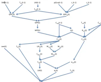
Figure 1.Variable dependencies and updating in SEDGES
SEDGES is a new model that is based on the original SIMulator for Biospheric Aspects (SimBA) model (Kleidon, 2006b), which is coupled to the Planet Simulator (PlaSim) general circulation model (GCM) (Lunkeit et al., 2007), and it is even more strongly based on a later version of SimBA that the lead author of this paper developed (Lunkeit et al., 2011) and which is also coupled to PlaSim. Neither version of SimBA has been thoroughly evaluated. However, when coupled to PlaSim, the earlier version’s net primary pro-ductivity was shown to be broadly reasonable in Kleidon (2006b), and it has been used successfully in a number of studies (e.g., Kleidon, 2006a, b; Bowring et al., 2014). The SimBA model is based on a light and water-use efficiency model for crops (Monteith et al., 1989) that was later adapted and expanded to forest canopies (Dewar, 1997). This ap-proach to vegetative productivity is maintained in SEDGES and helps form the core of the model. Other aspects of SEDGES’s structure that are particular to SEDGES (i.e., are uncommon in or absent from other models) are carried over from the original SimBA, including the determination of soil water-holding capacity and moist-soil leaf cover fraction by the amount of vegetation biomass (Fig. 1).
SEDGES builds upon SimBA by improving most of its parameterizations. Some of the updated and expanded model features are taken or adapted from currently existing mod-els. Although SEDGES makes many improvements upon the original SimBA, it is still a simple model; i.e., it is not of “in-termediate” complexity (cf. Willeit and Ganopolski, 2016).
Compared to the original SimBA, SEDGES (and the land surface framework that it presupposes) has four major in-creases in complexity: the separation of evapotranspiration into soil and vegetative components, the inclusion of aero-dynamic conductance in the formulation for carbon uptake by vegetation, full coupling of photosynthesis and transpira-tion through interactive canopy conductance, and soil organic carbon-dependent soil albedo. Choosing the appropriate level of complexity of represented processes within a land surface or dynamic global vegetation model often depends on the context in which the model is to be used and involves sub-jective weighting of trade-offs between increased accuracy and realism on the one hand and, on the other hand, robust-ness to the chosen values of poorly constrained parameters and model reliability in a wide range of situations (Prentice et al., 2015).
2 Model description: SEDGES 2.1 Overview of SEDGES
SEDGES is a simple, dynamic global vegetation model (DGVM). Within the context of the history of land surface modeling, the SEDGES framework (defined as SEDGES and the type of land surface model that it presupposes that it forms a part of) combines aspects of first- and third-generation models (Sellers et al., 1997; Pitman, 2003; Pren-tice et al., 2015), which include, respectively, the use of a simple single-layer “bucket” model for soil hydrology and the full coupling of photosynthesis and transpiration through interactive canopy conductance.
The intended main use of SEDGES is for it to be embed-ded within a land surface scheme and to thus help the land surface scheme simulate large-scale properties and behav-ior of the surface in which vegetation and soil play a role. These large-scale properties and behavior include interac-tions between the land surface and the atmosphere through simulated CO2, moisture, energy, heat, and momentum ex-changes. SEDGES either directly simulates or else provides the greater land surface scheme with the necessary variables. SEDGES also simulates ecological variables (e.g., biomass, soil organic carbon, forest cover fraction, leaf cover fraction) that are not directly used outside it by either the rest of the land surface scheme or by the atmosphere, but these ecolog-ical variables almost always have a downstream impact on the simulations of the aforementioned land–atmosphere ex-changes. SEDGES has been designed, in particular, for cou-pling with the Planet Simulator, and thus presupposes that the land surface scheme that it forms a part of be similar to that of PlaSim in its hydrology and scheme for surface evap-oration. This section presents, in detail, the SEDGES model formulations for its output ecological and land surface vari-ables, including their derivations.
Overall, sub-grid-scale heterogeneity is treated similarly in SEDGES as it is in the SLAM-1T (Simple Land-Atmosphere Mosaic – 1 Tile) configuration of CHASM (CHAmeleon Surface Model) (Desborough, 1999) and in the original Met Office Surface Exchange Scheme (MOSES) land surface scheme (Cox et al., 1999). Because of its need to couple with the Planet Simulator GCM, which uses a bulk aerodynamic formulation with a single tile (i.e., one surface type per grid cell), SEDGES handles sub-grid-scale hetero-geneity according to what is called the “average parameter” method (Giorgi and Avissar, 1997) or the “composite” ap-proach (Li and Arora, 2012; Melton and Arora, 2014). In this approach, land surface characteristics are aggregated to pro-vide a single, representative value on the scale of the entire grid cell. The framework in SEDGES for evapotranspiration (ET) is special because it also qualifies as a simplified mo-saic (or “mixed”, Li and Arora, 2012) approach, such that only surface conductance differs between the surface types (or tiles). This mosaic approach is also used to extend a
“big-rcu(t)
rc(t)
rcmin(t) GPPL(t) GPPW(t) rc(t-1) Tsfc(t-1) Tsfc(t) SW (t-1) SW (t) ra(t-1)
ra(t)
Wfrac(t)
PET(t)
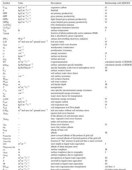
Figure 2. Canopy resistance dependencies and updating in SEDGES
leaf” formulation for vegetative CO2uptake (Appendix B of Raupach, 1998) to a mixed soil–vegetation surface, enabling us to isolate the fraction of total ET that is due to transpira-tion and thus formulate vegetative control of water loss and CO2uptake. The SEDGES framework neglects evaporation from intercepted canopy water and thus only distinguishes between two tiles when snow is absent: bare soil and vege-tation. When there is snow cover, there are essentially three tiles: snow-free exposed bare soil, snow-covered surface, and snow-free exposed vegetation (see Sect. 2.3.1 for more de-tail).
The core driving variable in SEDGES is gross pri-mary productivity (GPP), which impacts the living biomass, which, in turn, heavily influences or determines the values of almost every other simulated land surface variable (listed in Sect. 3). Forest cover and leaf cover fractions and (implicitly) rooting depth are parameterized to increase with biomass us-ing respective relationships that are fixed. SEDGES (as well as SimBA) uses a simple single-layer bucket for the soil hy-drology and has essentially one plant functional type. Soil organic carbon is treated as a single homogeneous reser-voir. Surface albedo depends on soil organic carbon content, snow depth, biomass, and leaf cover fraction. Surface rough-ness increases monotonically with biomass. Gross primary productivity and canopy resistance1are coupled through the vegetation’s effort to conjointly minimize water loss and sat-isfy photosynthetic demand for CO2, as per the original De-war (1997) model (see Sect. 2.2.6). Table 1 lists all SEDGES variables, their units, and their relationship with the SEDGES vegetation model. Their dependencies and how those vari-ables are updated is shown in Figs. 1 and 2. Table 2 lists all parameters that are used in the paper along with their values and their units.
1Canopy resistance and conductance are aggregated or “bulk”
Table 1.SEDGES variables in the paper. Notation for the rightmost column is as follows: “I”, “O”, and “M” indicate variables that are, respectively, input to, output by, or modified by the SEDGES model. A blank field in that column indicates that the variablecouldbe output if desired, but some code changes would be needed. “EI” denotes a variable from ERA-Interim that is used by the simple land surface scheme that we use to drive SEDGES with in Sect. 4. We denote by “M” only those output variables that are output by SEDGES that are expected to be already existing in the land surface scheme in which SEDGES is embedded.
Symbol Units Description Relationship with SEDGES
Cveg kg C m−2 vegetative carbon O
L kg C m−2s−1 litterfall O
NPP kg C m−2s−1 net primary productivity O
GPP kg C m−2s−1 gross primary productivity O
GPPL kg C m−2s−1 light-limited gross primary productivity O GPPW kg C m−2s−1 water-limited gross primary productivity O
f1(CO2) – CO2fertilization function
f2(Tsfc) – temperature limitation function O
Tsfc K surface temperature I
fAPAR – fraction of photosynthetically active radiation (PAR) that is absorbed by green vegetation
SW↓ W m−2 surface downwelling shortwave radiation I
LAI m2leaf area (m2ground area)−1 leaf area index O
fleaf – vegetative leaf cover fraction O
ga m s−1 aerodynamic conductance I
ra s m−1 aerodynamic resistance
rc s m−1 canopy resistance O
ρ kg m−3 surface air density I
psfc Pa surface pressure I
ET m3m−2s−1 evapotranspiration calculated outside of SEDGES
qsatsfc kg H2O kg air−1 surface saturation specific humidity calculated outside of SEDGES
q kg H2O kg air−1 specific humidity at the lowest atmospheric level EI
Cw – surface wetness factor M
βss – soil surface water stress factor
rss s m−1 soil surface resistance
Wfrac – soil wetness fraction
Wsoil m soil water content I
Wmax m soil bucket depth M
T m3m−2s−1 transpiration O
r∗cu s m
−1 case-specific unconstrained canopy resistance
rcu s m
−1 unconstrained canopy resistance
βtr – water stress factor for transpiration
rcmin s m−1 minimum canopy resistance O
Csoil kg C m−2 soil organic carbon O
Rsoil kg C m−2s−1 soil respiration rate O
Tsoil K soil temperature at 0.20 m depth I
LAIm m2leaf area (m2ground area)−1 leaf area index without soil moisture stress
fleafm – (green) leaf cover fraction
in the absence of soil moisture stress
fleafdry – max. vegetative leaf cover fraction
under soil moisture stress
ffor – forest cover fraction O
α0 – snow-free surface albedo
αsoil – albedo of bare soil
α – albedo M
αsnow flat – snow-covered albedo of flat portion of grid cell
αsnow for – snow-covered albedo of forested portion of the grid cell
fsnow flat – fraction of “flat” portion of grid cell that is snow-covered
swe m3m−2 snow depth in liquid water equivalent I
αdeep snow,flat – albedo of deep and pure snow
z0 m surface roughness M
z0oro m surface roughness due to orography I
z0veg m surface roughness due to vegetation
P m3m−2s−1 precipitation in liquid water equivalent EI
S m3m−2s−1 snowfall in liquid water equivalent EI
M m3m−2s−1 snowmelt in liquid water equivalent EI
ETsoil m3m−2s−1 bare-soil evaporation plus transpiration see Sect. 4
Esoil m3m−2s−1 bare-soil evaporation O (when snow present)
Table 2.SEDGES parameters in the paper.
Symbol Value Units Description Source(s)
τveg 10 years (converted biomass residence time SimBA (all versions)
into seconds)
Rd 287.0 J K−1kg−1 gas constant for dry air on Earth –
max 5.0×10⁻¹⁰ kg C J−1 max. light use efficiency model calibration CO2comp 40 ppmv CO2light compensation point Franks et al. (2013)
Tcrit 20 ◦C temperature at which see Sect. 2.2.3
productivity limitation begins
kveg 1 – light extinction coefficient see Sect. 2.2.3
c 0.7 – clumping index Pisek et al. (2010); He et al. (2012)
co2conv 4.15×10⁻⁷ kg C kg air−1ppmv−1 unit conversion factors manipulation of Eq. (B7) from Raupach (1998) ci
ca 0.80 – ratio of intercellular somewhat common daytime
to atmospheric CO2 value for C3 plants
rssmin 10 s m−1 minimum soil surface resistance van de Griend and Owe (1994)
rssmax 1030 s m−1 maximum soil surface resistance –
ρw 1000 kg m−3 density of liquid water –
fsnow for 0.12 – snow-covered fraction of the forest cover see Sect. 2.2.5 trmax 2.78×10⁻⁷ m s−1 max. transpiration rate Knorr (2000)
rcminmin 0 s m−1 absolute min. canopy resistance –
rcmax 1030 s m−1 max. canopy resistance –
c8 ≈43.3 (see – for normalizing 10◦C soil
Sect. 2.2.7) respiration to that of SimBA
c9 106 K for soil respiration Jenkinson et al. (1990)
LAImin 0.05 – min. leaf area index in wet soils –
LAImax 7 – max. leaf area index in wet soils model calibration
c6 0.195 kg C−1m2 biomass to LAI conversion model calibration
Wfraccrit,lai 0.05 – critical soil wetness fraction model calibration for commencement of leaf fall
c1 0.2 kg C−1m2 biomass–forest-cover relationship see Sect. 2.2.9
c2 1.0 kg C m−2 biomass threshold for see Sect. 2.2.9
forest cover commencement
c7 9 kg C m−2 soil organic carbon saturation value see Sect. 2.3.1 with respect to soil albedo
αsand 0.32 – sandy soil albedo see Sect. 2.3.1
αpeat 0.12 – albedo of organic-matter-rich soil see Sect. 2.3.1
c4 1.5 kg C−1m2 shape parameter for snow- model calibration
covered albedo
c5 1.5 kg C m−2 biomass threshold for model calibration
snow masking
αmin deep snow flat 0.40 – albedo of warm, deep, pure snow Roesch et al. (2001)
αmax deep snow flat 0.80 – albedo of cold, deep, pure snow Roeckner et al. (2003)
αmax snow for 0.30 – maximum albedo of snow- Moody et al. (2007) covered forest
c12 0.10 kg C1/2 conversion of biomass model calibration
into soil bucket depth
Wmaxmin 0.05 m minimum soil bucket depth see Sect. 2.3.2
z0min 0.01 m surface roughness for bare soil Oke (1987)
z0const ≈0.035 m biomass–roughness relationship see Sect. 2.3.3
c15 8 kg C m−2 biomass–roughness relationship model calibration
c16 0.5 kg C−1m2 biomass–roughness relationship model calibration
c17 2.5 m ≈ surface roughness typical value for tropical rain forests
With its main use and design already indicated, SEDGES can also be forced offline with external data. The offline mode of SEDGES was used in combination with a simple soil hydrological scheme and parameterization for aerody-namic conductance and run using reanalysis climate data for the SEDGES model evaluation (see Sect. 4).
In Sect. 2.2 and 2.3, we describe in detail the equations of the ecological and physical variables in the SEDGES model. Because SEDGES uses the original SimBA model (Kleidon, 2006b) (and its code) as a basis, we explicitly mention in the text when significant changes are introduced in SEDGES compared with SimBA. We provide extra detail on the origi-nal SimBA for the cases in which (Kleidon, 2006b) provides insufficient information for comparison with SEDGES. The broadest structural increases in complexity in SEDGES have already been identified in the introduction; our focuses are narrower in scope in these coming sections.
2.2 Equations for ecological variables 2.2.1 Vegetation biomass
The most important SEDGES variable is biomass of live veg-etation. This quantity is used to directly or indirectly derive almost all the land surface variables; these are presented in the coming sections. The prognostic equation for biomass is as follows:
dCveg
dt =NPP−L, (1)
where Cvegis the carbon in living biomass (kg C m−2),Lis the litterfall and equals Cveg
τveg,τvegis the residence time of the vegetative carbon (see Sect. 2.2.9) and equals 10 years, and NPP (net primary productivity) is approximated as 0.5 GPP. 2.2.2 Net primary productivity and gross primary
productivity
SEDGES uses a constant NPP/GPP=0.5 approximation. This approximation is supported by the conservative na-ture of the ratio of mitochondrial respiration to gross pho-tosynthesis and (hence) of the ratio of net phopho-tosynthesis to gross photosynthesis over a wide variety of conditions, on timescales of weeks or more (see the brief review in Van Oi-jen et al., 2010). Since each model time step in SEDGES is much shorter than this, it thus might seem incorrect to hold NPP/GPP fixed for each time step. It is appropriate to do so, however, because the NPP-to-GPP ratio in SEDGES only impacts biomass changes, and the latter occur on very long timescales. Finally, meta-analyses of previous studies have found a robust (DeLucia et al., 2007; Litton et al., 2007) linear or proportional relationship between NPP and GPP, with slope or proportionality constant of around 0.5 (Gif-ford, 2003; DeLucia et al., 2007; Litton et al., 2007), albeit with considerable variation in NPP/GPP across field sites
(Amthor and Baldocchi, 2001; DeLucia et al., 2007; Litton et al., 2007).
GPP is calculated as the minimum of a light-limited rate, GPPL, and a water-limited rate, GPPW(Monteith et al., 1989; Dewar, 1997). That is, GPP=min(GPPL,GPPW.)
2.2.3 Light-limited gross primary productivity
GPPL uses a light use efficiency (LUE) formulation (e.g., Yuan et al., 2007) whose overall structure is very similar to that of the original version of SimBA (Kleidon, 2006b). The equation is as follows:
GPPL=max·f1(CO2)·f2(Tsfc)·fAPAR·SW↓, (2) where max is a globally constant maximum LUE param-eter (5.0×10⁻¹⁰kg C J−1);f1(CO2)is a CO2 fertilization function (described below);f2(Tsfc)is a temperature limi-tation function (described below);fAPAR is the fraction of photosynthetically active radiation (PAR) that is absorbed by green vegetation (see below); and SW↓is the downward flux of shortwave radiation just above the canopy surface (in W m−2). (Instead of this term, the original version of SimBA (Kleidon, 2006b) uses the net surface shortwave radiation flux.)
In Eq. (2), the first term on the right-hand side,max, is the LUE with respect to the total shortwave broadband radiation that is absorbed by the photosynthetic parts of the vegetation. This constant term is the maximum efficiency with which in-cident shortwave radiation can be used to synthesize vegeta-tive carbon at the reference (360 ppmv) CO2level (also see explanation offAPAR, below).
The second term in Eq. (2),f1(CO2), increases productiv-ity with increasing CO2and is taken directly from Eq. (5) of Franks et al. (2013). For CO2>CO2comp, we have
f1(CO2)=CO2norm
ca−CO2comp ca+2CO2comp
, (3)
where ca is the atmospheric CO2 concentration (ppmv), CO2comp=40 ppmv is the light compensation point in the ab-sence of dark respiration, and CO2norm=360+2CO2comp
360−CO2comp . Oth-erwise,f1(CO2)=0. This fertilization function replaces an earlier “beta” factor approach used in SimBA (Lunkeit et al., 2011). The latter does not saturate and therefore yields unre-alistically large fertilization at high CO2levels.
The third term in Eq. (2) isf2(Tsfc).f2(Tsfc) is a ramp function, reducing productivity linearly from a surface tem-perature of Tcrit≡20 to 0◦C, with f2(Tsfc)=0 for below 0◦C temperatures. The 20◦C value is the critical tempera-ture below which productivity drops. See Appendix A for more discussion.
of incoming solar radiation that is in wavelengths usable for photosynthesis. We approximatefAPARas follows:
fAPAR=1−e−kveg·c·LAI, (4) wherekvegis a light extinction coefficient (set to 1 for hori-zontal leaves),cis the clumping index (or factor) and is set to 0.7, a near-mean value for natural land cover types (Pisek et al., 2010; He et al., 2012), and LAI is the leaf area index (see Sect. 2.2.8).
Equation (4) uses a simple Beer–Lambert approach, ex-tended to canopies with leaves that are nonrandomly dis-tributed in space (Nilson, 1971) (e.g., “clumped”). Here, we have used the common approximation (e.g., see Gower et al., 1999) that fAPAR equals the fraction of intercepted PAR (fIPAR). Other assumptions and simplifications in Eq. (4) include an azimuthally symmetric leaf distribution (Gower et al., 1999), leaf absorptivity of 1 with respect to PAR, and the neglect of the influence of non-photosynthesizing plant parts. A final and important assumption of horizon-tal leaves2 eliminates zenith angle dependency of the light extinction coefficient (Campbell and Norman, 1998), which makes the canopy gap fraction the same from any angle. This, in turn, eliminates the dependency offIPAR on diffu-sive/direct radiative partitioning and on zenith angle, thus re-ducing fIPAR (andfAPAR) to the simple Beer–Lambert ex-pression of Eq. (4), with a constant light extinction coeffi-cient. Earlier versions of SimBA and the derivative model (Dewar, 1997) assume a constant value of 0.5 forkveg.
The simplifications made in the last paragraph allow us to interchangefAPARand the leaf cover fraction,fleaf. Thus, we can rewrite Eq. (4) as follows:
fleaf=1−e−kveg·c·LAI, (5) wherefleaf is the areal fraction of view that is covered by photosynthesizing plant parts when looking directly down on the land surface. That is,fleaf=1−the gap fraction from the nadir.
2.2.4 Water-limited gross primary productivity
Most land plants take up the CO2they need for photosynthe-sis through tiny pores in their leaves called “stomata”. Water is also lost (transpired) through these same openings. Wa-ter loss in excess of waWa-ter uptake can lead to cavitation, hy-draulic system collapse (e.g., see discussion in Sperry et al., 2While spherical leaf angle distribution is commonly assumed
for unmeasured canopies, measurements of 58 temperate and bo-real broadleaf tree species showed planophile (tending toward hor-izontal) leaf angle distributions in 30 and spherical distributions in just 5 (Pisek et al., 2013). Moreover, a modeling study (Hikosaka and Hirose, 1997) used game theoretical arguments to show how a horizontal leaf angle distribution is to be evolutionarily expected, in general (save for canopies with high LAI and high self-shading). Thus, globally applying a horizontal canopy leaf distribution is not unreasonable.
2002), and/or permanent reduction in photosynthetic capac-ity (Lawlor and Cornic, 2002). To prevent and mitigate such occurrences in both the present and future, most land plants adjust their stomatal openings in such a way as to balance the short- and long-term costs of transpiration with the photosyn-thetic gain from increased CO2intake (Cowan and Farquhar, 1977; Medlyn et al., 2011; Buckley and Schymanski, 2014; Prentice et al., 2014). Thus, water limitation in most land plants is closely tied to CO2 limitation on photosynthesis. For this reason, this CO2-limited rate in SEDGES is referred to as the “water-limited rate of GPP”. This rate is given as follows:
GPPW=
(co2conv)1−ci
ca
ca(fleaf)ρ
1.6rc+ra , (6)
where rc is the canopy resistance (see Sect. 2.2.6); ra is the aerodynamic resistance; ρ≡ psfc
RdTsfc
is the sur-face air density, where psfc is the surface pressure and Rd is the gas constant for dry air; co2conv=4.15× 10⁻⁷kg C kg air−1ppmv−1;cirepresents a “bulk leaf” inter-cellular concentration of CO2(ppmv); and ccia is set to 0.80. This last value was lowered from the≈0.86 value that was apparently used in Raupach (1998) because such a high value is less representative of typical daytime ci
ca values (e.g., see Prentice et al., 2014). SimBA uses a value of 0.7. The rami-fications of using a fixed value of ci
ca are discussed in Sect. 6. Equation (6) is essentially the bulk aerodynamic formula for CO2in Appendix B of (Raupach, 1998), except that we have multiplied their right-hand side byfleaf to generalize from their big-leaf approach to the simplified mosaic frame-work (as mentioned in Sect. 2.1), and we have multiplied by the ratio of the molar masses of carbon and CO2to convert the flux into carbon units. In addition, we neglect the contri-bution of leaf mitochondrial respiration for simplicity. (It can be shown that including daytime leaf mitochondrial respira-tion in the formularespira-tion of GPPWmultiplies its current form by a factor of1−1X, whereXis the ratio of leaf mitochondrial respiration under light to gross photosynthesis.)
Latitude
Annual
Figure 3.Zonal multiyear monthly means and zonal multiyear annual means of ET for SEDGES and the Mueller et al. (2013) reference dataset for the 1989–2005 period over non-glaciated land.
aerodynamic formulation for GPPWalso unifies vegetation– atmosphere exchanges of CO2 and water under the same physical framework, which enables the process of transpira-tion to be properly tied into carbon uptake through interactive canopy conductance (see Sect. 2.2.6).
2.2.5 Evapotranspiration and transpiration
As was mentioned earlier in Sect. 2.1, the SEDGES frame-work for ET is very similar to the approaches taken by the SLAM-1T configuration of CHASM (Desborough, 1999) and by the original MOSES land surface scheme (Cox et al., 1999). These approaches all expand on the SimBA frame-work (Appendix C) by separating evapotranspiration into soil and vegetative components and (in SEDGES and MOSES) by coupling photosynthesis and transpiration through in-teractive canopy conductance. We find that these changes greatly improve the simulation of ET (compare Fig. A2 with Fig. 3) when using the forcing setup described in Sect. 4.
By design, SEDGES does not directly calculate the evap-otranspiration; rather, it provides a surface wetness factor to be used by the bulk aerodynamic formulation of the land sur-face scheme that is coupled to the atmospheric model, which performs the actual calculation of ET. An exception to this exporting of ET calculation to outside of SEDGES is the ex-plicit calculation by SEDGES of evaporation from exposed soil when there is snow cover.
Although the (total) evapotranspiration is calculated out-side of SEDGES, the way it is simulated is intimately tied into many parameterizations within the actual SEDGES model, which presuppose a specific ET framework (as dis-cussed in Sects. 2.1 and 3). The ET framework is thus pre-sented in this section, along with the SEDGES
parameteri-zations that help comprise it. For this simplified mosaic ap-proach (Sect. 2.1), we remind the reader that the aerodynamic conductance and saturation specific humidity of the air at the surface are homogeneous throughout the grid cell:3
ET= ρ
ρwra
Cw1q, (7)
where ET is the evapotranspiration in units of volumetric liquid water m3m−2s−1, ρw is the density of liquid wa-ter,1q≡qsatsfc−q,qsatsfc is the temperature- (Tsfc) and pressure- (psfc) dependent saturation specific humidity of the air at the surface,q is the specific humidity of the air at the lowest atmospheric model level, and Cw is a surface “wet-ness” factor that reduces evapotranspiration from the poten-tial rate by incorporating the effects of canopy resistance and soil resistance. Cwranges from 0 to 1, where “1” gives the potential evapotranspiration (PET) rate:
PET= ρ
ρw ra1q. (8)
Although the above framework for ET (and PET) is re-quired in order for SEDGES to operate as designed, there is no stipulation that the coupled land surface model calculate qsatsfc orrain any preset way. That said, it is desirable for 3In this paper, we define ET and transpiration (T) as positive
the calculation ofrato depend, in some way, on the surface roughness length that is output by SEDGES (Sect. 2.3.3).
Under snow-free conditions, SEDGES derives the key ET variable, the surface wetness factor, as follows:
Cw= fleaf 1+rcga
+ 1−fleaf
1+rssga
, (9)
wheregais the aerodynamic conductance4
= 1
ra
, andrssis the soil surface resistance, whose formulation is taken from the Joint UK Land Environment Simulator (JULES) model (Best et al., 2011), except for the use of the lower minimum soil resistance from van de Griend and Owe (1994). This re-duction was made to compensate for the absence of evapo-ration from ponded surface water in SEDGES. Soil surface resistance is formulated as follows:
rss=min
rssmax, rssmin
βss
, (10)
where rssmin is the minimum soil surface resistance of 10 s m−1(van de Griend and Owe, 1994),rssmax is the max-imum soil surface resistance (a very large number), andβss limits evaporation from the soil surface and is considered a “water stress factor”. This last factor is formulated according to (Best et al., 2011), except that SEDGES uses the entire soil hydrological layer instead of just the top of several lay-ers. The water stress factor for the soil surface in SEDGES is as follows:
βss=Wfrac2, (11)
where the soil wetness fraction,Wfrac, is given as follows: Wfrac=
Wsoil
Wmax, (12)
whereWmaxis the biomass-dependent soil bucket depth and Wsoil is the water content (as depth) within the bucket. The SimBA model uses a general water stress factor that is a ramp function, reducing ET linearly from a soil wetness fraction of 0.25 to 0. In SimBA, Cw is equal to this water stress factor. In this way, no distinction is made between soil moisture’s impact on soil evaporation and its impact on transpiration.
Examining Eq. (9), we see that Cwis comprised of a veg-etation term and a bare-soil term (since 1−fleafis the bare-soil fraction (neglecting non-photosynthesizing plant parts for simplicity)). The vegetation term involves loss of water only due to transpiration; canopy interception and evapora-tion are neglected for simplicity. Under snow-free condievapora-tions, ET is partitioned into transpiration and bare-soil evaporation, 4An important requirement for the aerodynamic conductance
formulation is that the surface roughness for moisture be the same as that for momentum. See Sect. 2.3.3 for more discussion.
respectively, by replacing Cw in Eq. (7) with the vegetation term, fleaf
1+rcga, or with the bare-soil term, 1−fleaf
1+rssga. Doing so with the vegetation term yields the following equation for transpiration:
T= ρ
ρw fleaf ra+rc
1q. (13)
From the above formulations, one can see that we weight the contributions to evapotranspiration from transpiration and bare-soil evaporation, respectively, by the fractional cov-erages of vegetation and bare soil.
In the presence of snow cover, the surface is treated as a mosaic of different types, with each type sharing the same aerodynamic conductance, soil hydrology, and surface tem-perature, as discussed before (Sect. 2.1). The parts of the grid cell that are snow-covered evaporate at the potential rate. The portion of the grid cell considered to be snow-free surface is comprised of vegetation parts that protrude above the snow-pack and are snow-free, the exposed bare soil, and the ex-posed, low-lying leaf cover. In these snow-free portions of the grid cell, transpiration is 0 and bare-soil evaporation oc-curs (Eqs. 7, 9, and 10). The final equation for Cw in the presence of snow in the grid cell is as follows:
Cw=
(1−ffor)(1−fleaf)(1−fsnow flat) 1+rssga
(14)
+(1−ffor)(fsnow flat)+(ffor)(fsnow for),
wherefforis the forest cover fraction (Eq. 23),fsnow flatis the fraction of the flat portion of the grid cell that is covered by snow (see Eq. 27 and nearby text), andfsnow for≡0.12 is the snow-covered fraction of the vegetation cover that protrudes above the snow pack (i.e., of the forest cover).5
From Eq. (14) and the relationship ET=CwPET (from Eqs. 7 and 8), one can deduce that bare-soil evaporation, Esoil, when there is snow cover is given as follows:
Esoil=
(1−ffor)(1−fleaf)(1−fsnow flat) 1+rssga
PET. (15)
In SimBA, Cw=1 when there is snow cover. The formu-lation was changed in SEDGES when it was discovered that it led to excessive ET when snow was present. The original MOSES and its progenitor UKMO (United Kingdom Met Office) scheme also set their equivalent Cwto 1 when there is snow cover, which also leads to excessive ET under those conditions (Essery, 1998; Cox et al., 1999).
5The value of 0.12 is a crude estimate that is obtained by
as-suming an albedo transition for forest vegetation from snow-free vegetation albedo to deep and cold snow albedo (0.80) that is linear withfsnow for. Depending on whether one uses values of 0.30 and
2.2.6 Canopy resistance
Canopy resistance,rc, is determined at each time step in ac-cordance with the supply/demand principle in the original (Dewar, 1997) paper. That is, the plants attempt to adjustrc so that CO2uptake exactly matches the light-limited rate of canopy photosynthesis, GPPL. (GPPLis the rate of gross car-bon uptake in the absence of any CO2limitation.) However, rcmust also be sufficiently high to prevent transpiration from exceeding the maximum rate suppliable by the roots (the “supply rate”). If thercvalue that would be needed to satisfy the CO2demand caused the transpiration to exceed the sup-ply rate, then water/CO2 limitation occurs andrc takes on the value that would yield transpiration at the supply rate. In the derivation of the equation for canopy resistance, the un-constrained adjustment ofrcis the first step. The second step is the calculation of the minimum possible value of rcthat satisfies the supply constraint on transpiration. If needed, the unconstrainedrcis raised to this minimum value.rcis also constrained to not exceed a maximum possible value,rcmax. Details on the mechanics of the formulation are given in Ap-pendix B.
The original SimBA model does not explicitly consider canopy resistance. Although the incorporation of an interac-tive canopy resistance scheme within a coupled water/CO2 exchange framework adds complexity to SEDGES, we feel that this is a critical feature for a vegetation model to have when it is used as part of a land surface model. In particular, significant climatic impacts of stomatal closure induced by increased CO2are well-established in the literature and in-clude reductions in ET, increased runoff, and increased sur-face temperature (Sellers et al., 1996a; Betts et al., 1997; Levis et al., 2000; Betts et al., 2007; Cao et al., 2010).
2.2.7 Soil organic carbon
The overall modeling framework for soil organic carbon is the same as that of both the original SimBA (Kleidon, 2006b) and the land surface component (ENTS) of GENIE (Grid Enabled Integrated Earth System Model) (Williamson et al., 2006). In this simple framework, soil organic carbon is treated as a single homogeneous reservoir (in which litter is included) that has a single, temperature-dependent residence time. Soil respiration (see below) depends only on tempera-ture. The prognostic equation for soil organic carbon is given by
dCsoil
dt =L−Rsoil, (16)
where Csoil is the soil organic carbon (kg C m−2),Lis the litterfall (Eq. 1), and Rsoil is the rate of soil respiration (kg C m−2s−1).
Soil respiration is modeled according to the following equation:
Rsoil=
c8Csoil τsoil
1+e
c9 Tsoil−254.85
, Tsoil>256.1 K,
0, Tsoil≤256.1 K,
(17)
whereTsoil is the soil temperature at ≈0.20 m depth (i.e., the middle depth of the topsoil layer in PlaSim),τsoil is the residence time (42 years) of the soil organic carbon at 10◦C, c8≡1+e
106
283.15−254.85, andc9=106 K.
The above formulation is based on that of ENTS (Williamson et al., 2006), except that we replace its temper-ature dependency (Lloyd and Taylor, 1994) with that from the RothC (Rothamsted Carbon Model) soil organic carbon model (Jenkinson et al., 1990; Clark et al., 2011), since the latter’s temperature function reduces a negative soil organic carbon bias in the high Arctic. In addition, we usec8as a nor-malizing constant to make the soil organic carbon residence time, Csoil
Rsoil, at 10
◦C the same as in the original SimBA
for-mulation. Moreover, for strictly numerical purposes, 256.1 K is used as the cutoff temperature, below which soil respi-ration is set to 0. In SimBA, soil respirespi-ration is parameter-ized as follows:Q10
Tsfc−10 10
C
soil
τsoil. (Here, theTsfc is surface temperature in◦C, and Q10 is set to 2). In the current ver-sion of SEDGES, it is tacitly assumed, for simplicity, that all respired soil organic carbon is emitted directly to the atmo-sphere.
2.2.8 Leaf area index and leaf cover fraction
LAI is typically defined as “the one-sided leaf area per unit ground area”, or else, for conifers, as the projected area of the needle leaves (Monson and Baldocchi, 2014, p. 246). In SEDGES (as well as in SimBA), LAI is based on a moist soil value that gets subsequently reduced for conditions of low soil moisture. We first describe the moist soil formulation.
For sufficiently moist soils, LAI is a simple function of biomass. In the version of SimBA that came out with version 15 of the Planet Simulator model (Lunkeit et al., 2007), this moist soil LAI is a linear function of forest cover fraction (which, in turn, depends directly on biomass). This param-eterization is discarded in the subsequent SimBA in version 16 of Planet Simulator, in favor of a simpler LAI functional dependency on biomass (Lunkeit et al., 2011) to reduce the high number of multiple equilibria in the coupled climate-vegetation system that Dekker et al. (2010) found when using PlaSim version 15. This new parameterization is maintained in SEDGES, but its three parameters have updated values.
The equation for LAI in the absence of soil moisture stress is a monotonically increasing function of biomass with de-creasing slope:
LAIm=LAImin+ 2
where LAIminand LAImaxare the minimum and maximum LAIs (respectively) under moist soil conditions. LAIminis set to 0.05 and represents a seeding source with negligible mass. LAImaxis set to 7.
While winter-deciduous phenology is not included in SEDGES, the model simulates drought-deciduous phenol-ogy using a crude parameterization from SimBA that came originally from the ECHAM3 model (Klimarechenzentrum, 1993). LAImis converted into leaf cover fraction,fleafm, by substituting it into Eq. (5), giving the following:
fleafm=1−e
−kveg·c·LAIm, (19)
wherefleafmis the leaf cover fraction under moist soil condi-tions.
Then, we set
fleaf=min(fleafm, fleafdry), (20) where
fleafdry=
1, Wfrac≥Wfraccrit,lai, Wfrac
Wfraccrit,lai
, 0< Wfrac< Wfraccrit,lai, 0, Wfrac=0.
(21)
Here,fleafdryrepresents the maximum leaf cover permitted by the soil wetness fraction;Wfraccrit,laiis the critical soil wetness fraction at which leaf cover begins to get restricted and is set to 0.05.
Although the final LAI is merely a diagnostic, it has a one-to-one relationship withfleafbecause thefleafin Eq. (20) is converted back into LAI by inverting the LAI–fleaf relation-ship in Eq. (5) as follows:
LAI=−ln(1−fleaf)
kveg·c
. (22)
2.2.9 Forest cover fraction
In SEDGES, forest cover fraction is defined as the fraction of the grid cell above ground that is covered by trees. How-ever, woody shrubs are counted as partial trees. It has no sea-sonal phenology. Forest cover fraction helps to determine the amount of surface that is covered by snow for the calcula-tion of evaporacalcula-tion (see Eq. 14). In SimBA, forest cover af-fects the albedo of snow-covered land; instead, SEDGES has a dependency on biomass (Eq. 26). As in the last version of SimBA (Lunkeit et al., 2011), forest cover is parameter-ized to commence at a biomass of 1 kg C m−2. Such cover would represent woody shrubs. Only at a biomass threshold of 1.5 kg C m−2is the woody cover considered tall enough so as to protrude above the winter snowpack and lower the albedo (Sect. 2.3.1). Forest cover fraction is formulated as follows:
ffor=max0,1−e−c1(Cveg−c2), (23)
wherec1is a shape parameter andc2is the biomass threshold for forest cover.
The derivation of thec1andc2parameter values involved translating NPP from outside data into SEDGES biomass. If one assumes long timescales and steady-state conditions, then the translation is readily achieved by setting the left-hand side of Eq. (1) to 0 and solving for Cvegin terms of NPP. Doing so results in the following relationship: NPP=Cveg
τveg. Using this relationship allows modeled annual NPP from Cramer et al. (1999) and McGuire et al. (1992) to be inter-preted as SEDGES biomass equivalent. Then, comparing the real-world spatial distribution of boreal forest, boreal wood-land, and tundra with the NPP data in those sources, includ-ing the NPP ranges for boreal forest, boreal woodland, and tundra ecosystems in McGuire et al. (1992), yields a rough threshold value of 1 kg C m−2 for forest cover commence-ment. The shape parameter,c1, was tuned so that forest cover fraction values in the Hagemann (2002) land cover dataset would match the NPP values in Cramer et al. (1999) for natu-ral land cover types, while maintaining a fairly close likeness between the SEDGES-parameterized and Hagemann (2002) relationships between forest cover fraction and LAI. (This likeness was assessed by scatterplotting the forest cover frac-tion and maximum LAI for the moist ecosystems given in Hagemann (2002) along with SEDGES-formulated forest cover fractions and LAIs for a wide range of biomass val-ues.) The original SimBA’s (Kleidon, 2006b) dependency of forest cover fraction on biomass uses an S-shaped curve that is equivalent toffor=max(0,atan(Cveg−3)−atan(−3))
0.5π−atan(−3) and is
sim-ilar to the formulation in the later SimBA version (Lunkeit et al., 2011). The two previous SimBA formulations give higher forest cover fractions than SEDGES except at some low biomass values. Neither SimBA parameterization yields a good match with the aforementioned reference data in the absence of using additional fitting parameters.
2.3 Equations for remaining land surface variables While the equations for the ecological variables were pre-sented in Sect. 2.2, here, we provide the formulations for the land surface variables used by the PlaSim GCM as well as some purely diagnostic variables.
2.3.1 Surface albedo
of the same form as that for SimBA, the ECHAM5 GCM (Rechid et al., 2009) and the ENTS land surface scheme (Williamson et al., 2006); it is as follows:
α0=αvegfleaf+αsoil(1−fleaf), (24) whereαvegis the albedo of a completely leaf-covered surface andαsoilis the albedo of the bare soil.
Soil albedo decreases linearly with soil organic carbon to a minimum value that is reached at 9 kg C m−2and stays con-stant with further carbon increase. The equation is as follows:
αsoil=
αpeat−αsand
c7 Csoil+αsand, Csoil≤c7, αpeat, Csoil> c7,
(25)
wherec7=9 kg C m−2 and is the soil organic carbon level at which the soil albedo saturates,αsandis the soil albedo in the complete absence of soil organic carbon, andαpeatis the albedo of soil when saturated with soil organic carbon.
This soil albedo formulation is taken from ENTS (Williamson et al., 2006), except for the following modifica-tions: the peat albedo has been increased from 0.11 to 0.12, the sand albedo has been increased from 0.30 to 0.32, andc7 was decreased from 15 to 9 kg C m−2. The first change was made for the sake of model simplicity (since the albedo of a fully leaved surface is 0.12 in SEDGES); the increase in sand albedo was made to better match observed values in the Sa-hara and Arabian deserts (e.g., Knorr and Schnitzler, 2006). A saturation level for soil albedo as a function of soil col-umn carbon content was estimated to be around 9 kg C m−2 by visually comparing the soil/litter surface albedo map from (Houldcroft et al., 2009) with a global gridded dataset of soil organic carbon content (Wieder et al., 2011). Using this es-timate for saturation value in SEDGES reduces a positive albedo bias in the high Arctic in summer as compared to us-ing the standard ENTS value of 15 kg C m−2.
The soil albedo formulation in SEDGES is an advent to SimBA, which has always used a fixed soil albedo of 0.30. The new dynamic scheme was adopted, in part, due to the important role played by ground albedo in Sahelian/Saharan vegetation–precipitation feedbacks, as seen through its effect on low-frequency precipitation variability (Vamborg et al., 2014) and increased greening in the mid-Holocene (Vam-borg et al., 2011). The new scheme also gives more realis-tic snow-free albedo values in the high latitudes and in the hot deserts (Fig. 4). While the above formulation for snow-free albedo, α0, neglects, for simplicity, the radiative im-pact of non-photosynthesizing plant parts (e.g., stems and branches), this impact becomes important (although implicit) in the snow-covered formulation.
A new snow albedo scheme for SEDGES replaces the ver-sion from SimBA that linearly combines the albedos from the forested and flat portions of the grid cell according to the for-est cover fraction. The SimBA formulation did not simulate well the sharp, real-world transition in snow-covered albedo
from tundra to boreal forest (Loranty et al., 2014), which is why a new exponential decay scheme was developed.
In SEDGES, for snow depth>0, the surface is treated as consisting of two components: (1) “flat” surface (consisting of exposed soil, prostrate vegetation, and dwarf shrubs) that can be partially or entirely buried by the snow cover; (2) “for-est” that is covered by trees and shrubs of sufficient stature so as to protrude above the snowpack and mask it from the sun via their leaves, stems, and/or branches, regardless of accu-mulated snow depth on the ground. A nonlinear combination of the albedo of the flat portion and the snow-covered forest albedo yields the final surface albedo (α):
α=αsnow for+(αsnow flat−αsnow for)e−c4·max(0,Cveg−c5), (26) wherec4is a shape parameter, andc5is the biomass thresh-old (1.5 kg C m−2) at which the woody vegetation is suffi-ciently tall as to begin to mask the snow.
The albedo of the flat portion of the grid cell,αsnow flat, is formulated according to the same temperature dependency (Roeckner et al., 2003) and snow cover fraction (Roesch and Roeckner, 2006) schemes for non-forested areas in the ECHAM5 model, except that we maintain the melting snow albedo of 0.4 from PlaSim and ECHAM4 (Roesch et al., 2001) and we neglect the impact of sloping terrain. We thus have the following:
αsnow flat=α0+(αdeep snow,flat−α0)·0.95fsnow flat, (27) where fsnow flat≡tanh(100 swe) is the fraction of the flat portion of the grid cell that is covered by snow (swe is the snow depth in liquid water equivalent (m3m−2)),6 and αdeep snow,flatis the albedo of a deep and pure snowpack and is temperature dependent. This dependency has the form of a ramp function, with a maximum albedo,αmax deep snow flat≡ 0.8, for surface temperatures ≤ −5◦C and a minimum albedo,αmin deep snow flat≡0.4, at melting point. These values are the same as in PlaSim and SimBA, except that they have maximum albedo attainment at−10◦C.
The albedo of the forest component of the grid cell when there is snow cover is as follows:
αsnow for≡min(αsnow flat, αmax snow for). (28) Here,αmax snow for is the maximum snow-covered albedo for forest and is set to 0.30, a midrange white-sky albedo value for the different forest types (Moody et al., 2007). Restricting αsnow for to not exceed αsnow flat is done because the lower snow depth and warmer snow that reduce the albedo of the flat area also lower the albedo of the forested area to at least the level of the flat area.
6Roesch and Roeckner (2006) include the 0.95 multiplier in
their definition of the snow-covered fraction of the non-forested part of the grid cell, but we do not. Note, too, that this scheme for non-forested snow cover fraction supplants the ECHAM4 pa-rameterizationfsnow flat=sweswe+0.01
(a) (b)
Figure 4. (a)SEDGES monthly mean climatologies of surface albedo for 2001–2010.(b)MODIS monthly mean climatologies of white-sky albedo for 2001–2010 (NASA LP DAAC, 2008b).
2.3.2 Soil bucket depth
We first introduced the soil bucket depth,Wmax, in Sect. 2.2.5 in Eq. (12). SEDGES uses a simplified version of the param-eterization in the JeDi (Jena Diversity) dynamic global veg-etation model (Pavlick et al., 2013). The JeDi model uses a pipe representation of the rooting system (Shinozaki et al., 1964) in which a square root relationship emerges between
Wmaxand coarse root biomass as a result of an assumed con-stant density of fine roots in the rooting zone. To adapt this formulation to SEDGES, we further assume that coarse root biomass is a fixed fraction of total biomass and that the unit plant-available water capacity is spatially constant. Doing so gives the following relationship:
Wmax=minWmaxmin, c12
q
Cveg
where c12 is a tuning parameter set to 0.10 kg C1/2. This value yields soil bucket depths that are a reasonably good fit with a plant-available water dataset based on optimal rooting depths (Kleidon and Heimann, 1998; Hall et al., 2006; Klei-don, 2011). In that dataset, the soil bucket depths in the most sparsely vegetated regions range from around 0.05 m in the Canadian polar desert to<0.003 m in the hyperarid Atacama and northeast Sahara deserts. SEDGES adopts a minimum soil bucket depth,Wmaxmin, of 0.05 m.
The versions of SimBA (Kleidon, 2006b; Lunkeit et al., 2007, 2011) computeWmaxusing the following formulation: Wmax=Z×Wmaxmax+(1−Z)Wmaxmin, whereZis the for-est cover fraction formulation in the original SimBA (see Sect. 2.2.9) andWmaxmax is some maximum value forWmax. ThisWmaxformulation was updated in SEDGES because the new formulation has the advantage of being derived from first principles (Pavlick et al., 2013).
2.3.3 Surface roughness
SEDGES has been designed for use in land surface schemes in which the surface roughness lengths for momentum and water vapor are the same (e.g., schemes that use parame-terizations from Louis, 1979; Louis et al., 1982). As such, SEDGES returns only a single value for surface roughness length, z0, for a grid cell. The (total) surface roughness is comprised of a surface roughness due to orography and a surface roughness due to vegetation:
z0= q
z0veg2+z0oro2, (30)
where z0oro is the orographic surface roughness and z0veg is the roughness due to vegetation. z0oro is used by some GCMs (including Planet Simulator) to account for the en-hancement of surface drag due to sub-grid-scale topographic variation (e.g., see Beljaars et al., 2004). z0oro is set to 0 by default because small-scale orographic variation has little effect on land-to-atmosphere moisture transfer (Huntingford et al., 1998; Blyth, 1999).
In the SimBA formulation, surface roughness due to veg-etation is parameterized assuming that only forest cover in-creases it appreciably and that prostrate vegetative cover does not. As such, sparsely vegetated surfaces are assigned too high of a surface roughness. SimBA has minimum and max-imum values of z0veg of 0.05 and 2 m, respectively (Klei-don, 2006b; Lunkeit et al., 2007, 2011). SEDGES replaces SimBA’s linear dependency ofz0vegon forest cover fraction with the following logistic curve that depends on biomass rather than forest cover fraction:
z0veg= c17
1+e−c16(Cveg−c15)
−z0const, (31)
wherez0const≡ c17
1+e−c16(−c15) −z0minis a constant (in meters) that forcesz0vegto equalz0minat zero biomass. The new for-mulation forz0vegis tuned by adjustingc15 andc16 so as to
roughly match reference values in the literature for differ-ent land cover types (especially those in Hagemann, 2002). z0min is set to a bare-soil value of 0.01 m (Oke, 1987).c17 represents the approximate maximum value ofz0vegand is assigned a value of 2.5 m, which is representative of tropi-cal rain forests (Sellers et al., 1996b).z0veg values that lie between these two extremes have been constrained by using the NPP–biomass relationship described in Sect. 2.2.9 and by visually comparing reference NPP and GPP values (Cramer et al., 1999; Jung et al., 2011), biome/land cover distribution maps (Ramankutty and Foley, 1999; Olson et al., 2001), and the aforementioned literature values ofz0veg for those land cover types.
3 How to couple SEDGES
As stated in Sect. 2.1, SEDGES is a DGVM and is to be em-bedded within a land surface scheme of a climate or Earth system model. As such, the input and output variables for SEDGES are not the same as those for the land surface scheme that SEDGES forms a part of because SEDGES has its own set of exchanges with the rest of the land surface scheme in which it lies.
At minimum, the following time-varying input fields are required by SEDGES: aerodynamic conductance (ga), surface temperature (Tsfc), surface downwelling (broad-band) shortwave radiation (SW↓), soil temperature at
≈0.20 m (Tsoil), (bulk aerodynamic) potential evapotranspi-ration (PET), soil moisture content (Wsoil), surface pressure (psurf), and snow depth water equivalent (swe). Most of these variables are either calculated by or made accessible to fully fledged land surface schemes.
Other variables that are used by SEDGES will usually be part of the land surface scheme and depend on additional in-put variables (not listed in the previous paragraph). This is also the case when using ERA-Interim (ECMWF Reanaly-sis – Interim) data to force SEDGES (Sect. 4). In addition, the following parameter values (see Table 2) are not specified within the actual SEDGES code, which means that they must be declared and assigned values either in outside modules (e.g., in the non-SEDGES part of the land surface scheme) or by modifying the current SEDGES code:max, atmospheric CO2 concentration (ca), the gas constant for dry air (Rd), maximum transpiration rate (trmax), and residence times for vegetative and soil organic carbon at 10◦C (τvegandτsoil).
productiv-ity (GPPL), temperature limitation function (f2(Tsfc)), water-limited gross primary productivity (GPPW), litterfall (L), and soil respiration (Rsoil).
In general, the land surface modeling framework that SEDGES presupposes must be reconciled with that of the land surface scheme of the Earth system or climate model that one is incorporating SEDGES into. In particular, in the absence of modification to either SEDGES or the original land surface scheme, the simulation of evapotranspiration ac-cording to the simplified mosaic and bulk aerodynamic for-mulations described in Sect. 2.1 and 2.2.5 is required. The requirement arises because the water and CO2 exchanges predicted through this framework are presupposed by the canopy resistance equations. The simplest and recommended scenario with regards to reconciling soil hydrology is that the land surface scheme use a single-layer bucket model because this is what SEDGES “sees” when calculating soil surface and canopy resistances. As an example, Eq. (32), used in our forcing of SEDGES with ERA-Interim data (Sect. 4), gives the standard hydrological formulation for the simple single-layer bucket model.
In the likely scenario that the original land surface scheme of the Earth system or climate model does not perfectly match the framework used by SEDGES, it should, in many cases, be easy to achieve consistency of frameworks by adapting SEDGES and/or the original land surface scheme. Such adaptation would be easiest for the case in which the land surface scheme uses a single or multiple tile/mosaic ap-proach because this apap-proach could be converted to the sim-plified mosaic framework of SEDGES by, at each time step, replacing tile surface temperatures and soil wetness frac-tions with their respective grid-cell-weighted averages and by computing an effective surface roughness for the grid cell (e.g., Mason, 1988) in the case of significant areal water body coverage.
Finally, many land surface schemes distinguish between a surface roughness length of water vapor and heat from a sur-face roughness length of momentum, which is done to correct the typical bulk aerodynamic formulation for its replacement of temperature at the height of the roughness length with sur-face temperature (e.g., see discussion and references in Chen et al., 1997a). Although SEDGES only computes a rough-ness length of momentum, there are many ways to convert this roughness length to the roughness length for vapor/heat (e.g., see analyses and references in Chen et al., 2010).
An advantage of SEDGES is that (at least in principle) it can be run at any horizontal and temporal resolution. How-ever, we encourage users to run the model using a sub-daily time step so that the generally positive diurnal covariances of light, temperature, aerodynamic conductance, and surface-to-air specific humidity difference can be adequately cap-tured. These covariances should increase ET, overall. On the other hand, if users choose a daily time step or longer, then they should also anticipate an increase in vegetative produc-tivity in water-limited regions due to the concomitant
reduc-tion in water stress. This reducreduc-tion in water stress can be off-set by decreasing trmax, the maximum transpiration param-eter (Appendix B).
4 Forcing SEDGES with ERA-Interim data
In this section, we describe the process by which we force SEDGES using an external forcing dataset, with the goal of evaluating the capability of SEDGES as part of a land sur-face model. Repeated 1981–2010 6-hourly data from ERA-Interim (Dee et al., 2011) are used as the driver. The follow-ing required forcfollow-ing variables (Sect. 3) were obtained from the reanalysis for direct input to SEDGES: surface (skin) temperature, surface downwelling shortwave radiation, tem-perature of the second-from-top soil layer, surface pressure, and snow depth water equivalent. Shortwave downwelling surface radiation is derived as follows: 3-hourly periods are isolated, and the two periods that straddle each given time (e.g., 12:00 Z straddled by the 09:00–12:00 Z and 12:00– 15:00 Z periods) are averaged to give the flux at that time. A glacier mask is derived by considering any land point that has a daily mean snow depth always greater than zero to be glaciated. No vegetation occurs on glaciated grid points. Fi-nally, all ERA-Interim data are interpolated to T62 resolution using climate data operators (CDOs) before being read into SEDGES.
In order to evaluate the performance of SEDGES, it is necessary to simulate soil hydrology in an interactive way rather than relying on soil moisture content from the external forcing dataset. (Early versions of SEDGES that were forced using reanalysis soil moisture resulted in unrealistic simula-tions of vegetation, especially in dry regions.) In order to do so, other land surface modeling components are combined with SEDGES, such that these components incorporate hy-drologically relevant SEDGES output (namely, Wmax, Cw, bare-soil evaporation (in the presence of snow), andz0) and provide SEDGES with the variables needed:ga, PET, and Wsoil.
of the following formulation to simulate soil moisture: 1Wsoil
1t =P −S+M−ETsoil, (32)
whereP is precipitation,Sis the rate of snowfall, andMis the rate of snowmelt (all in liquid water equivalent). Again, Wsoil cannot be greater than Wfrac, with any excess going into runoff. Here, ETsoilis the combined soil evaporation and transpiration (and thus not coming from the snow cover). Re-call from Sect. 2.2.5 that when there is snow cover, soil evap-oration (Esoil) is calculated by SEDGES. Under conditions of sufficient snow cover (see below for more), transpiration is 0 and ETsoilreduces from being the (total) ET to being Esoil.
Soil hydrology in the framework we have constructed for driving SEDGES requires careful treatment in the presence of non-zero snow depths. Such care is especially needed be-cause of the Tiled ECMWF Scheme for Surface Exchanges over Land (TESSEL) that is used by ERA-Interim and the data interpolation to the coarse T62 grid. The underlying TESSEL tile scheme and the spatial interpolation imply that data for a given grid cell that are fed into SEDGES can be physically inconsistent in the SEDGES framework (Sect. 2.1). The inconsistency arises because a grid cell can have a non-zero snow depth and yet have a homogeneous (as required and seen by SEDGES) surface temperature that is well above 0◦C. This situation, in the absence of any mod-ification to the SEDGES code, gives rise to common occur-rences in which there is substantial transpiration from snow-covered leaves and in which snow-snow-covered vegetation and ground are evaporating as if their surface temperatures were well above freezing. These occurrences are not only unphysi-cal; they give rise to higher simulated ET from a given snowy, above-freezing region than would occur over the same region if it were divided up into its original small, homogeneous but differing tiles.
A second issue that must be addressed when there is snow is the tendency for ERA-Interim to overpredict freezing rain at the expense of snowfall (Dutra et al., 2011). Because we treat rain as entering the soil without interception by the snowpack (as is done in the TESSEL land surface model; Dutra et al., 2010), the freezing-rain bias led our early sim-ulations to have an unrealistically large recharge of soil wa-ter reservoirs in winwa-ter in many locations, even though sur-face temperatures were well below 0◦C. The handling of the aforementioned snow-temperature inconsistency and the freezing-rain bias are discussed next.
In order to simply resolve the above issue of snow with above-freezing temperature, we separate possible conditions into two cases: (1) swe>snow thresh and (2) swe≤snow thresh, where we define snow thresh as the swe threshold above which the surface is treated as snow-covered with re-spect to evaporation from and the physiology of vegetation and the threshold at or below which the surface is treated as snow-free. In case 1, we assume that transpiration is negli-gible (due to combined cold temperature and physical
cover-age of leaves by snow) and thus introduce a slight modifica-tion to Eq. (2), by settingf2(Tsfc)to 0 (its value at freezing), which, in turn, forces the productivity to 0. In case 2, we as-sume that evaporation from snow is negligible, andf2(Tsfc) is as normal. Finally, we address the excessive partitioning of precipitation into liquid form at subfreezing temperatures by further assuming for case 1 that soil moisture cannot in-crease unless there is some snowmelt during the same time step. Snowmelt indicates the presence of above-freezing tem-peratures and, thus, the presence of liquid water that does not freeze on contact with the surface and can thus infiltrate into the soil.
5 Model evaluation
In this section we evaluate SEDGES as part of the simple hydrological scheme described in Sect. 4, forced with ERA-Interim data. We emphasize the results from the simulation forced with historical CO2, using reference datasets of veg-etative carbon, LAI, surface albedo, tree cover fraction, soil organic carbon, GPP, and evapotranspiration.
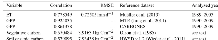
Four simulations are carried out: three equilibrium sim-ulations and one transient simulation. In the three equilib-rium simulations, atmospheric CO2 levels of 280, 360, and 560 ppm are held fixed through the simulations. The vegeta-tion is spun up from a vegetative and soil organic carbon-free state. The spin-up includes an acceleration of the carbon cy-cle for the first 260 years (only). From simulation year 261 to year 1500, the carbon cycle is run normally. The model is very nearly at equilibrium by the last 30 years in all three runs, and these years are thus analyzed. The transient simu-lation begins with the end state of the 280 ppm equilibrium simulation and is subsequently forced using observed, tran-sient atmospheric CO2values from 1832 to 2010. The CO2 data are taken from the Mauna Loa dataset (Keeling et al., 1976) for 1959 and onward and from 20-year smoothed ice core data (Etheridge et al., 1998) for the prior years. Un-less stated explicitly, the results and analyses always refer to the transient CO2 simulation. The model performs rea-sonably well, overall; GPP is simulated exceptionally well. In the evaluation process, we concentrate on the comparison of SEDGES with observation-based data products, but we sometimes supplement these comparisons with comparisons to land surface models and their performances, especially to the ENTS model (Williamson et al., 2006) because it is of similar complexity to SEDGES.
5.1 Evaluation of productivity
Latitude
Figure 5.Zonal multiyear annual mean of GPP for SEDGES and the two reference datasets, MTE and CARBONES, for 1990–2009 over non-glaciated land.
the model intercomparisons of Sitch et al. (2008), Piao et al. (2013), and Anav et al. (2015) and modeling-based results of Hemming et al. (2013) and Holden et al. (2013) to assess the relative performance of SEDGES.
For the 1982–2008 period, SEDGES simulates a global mean annual GPP of 126 Pg C yr−1 as compared to 120 Pg C yr−1for the observation-based MTE dataset (Jung et al., 2011). Zonal means of GPP, taken over the glacier-free land mask obtained from the ERA-Interim data and for 1990–2009, are shown for SEDGES, MTE, and the CAR-BONES data assimilation dataset in Fig. 5. SEDGES cap-tures the large-scale patterns very well. Compared to the two reference datasets, SEDGES has positive productivity biases in most of the Southern Hemisphere and around 35◦N, and
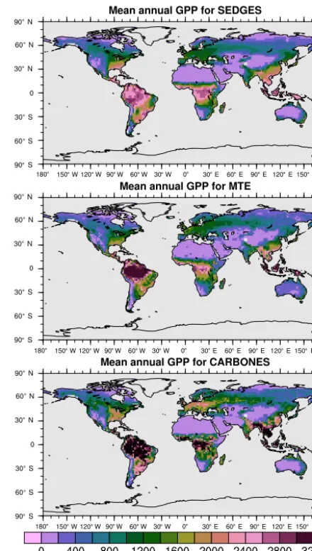
it has negative biases near the equator and in the high north-ern latitudes. Moving to the full spatial field, we can see in Fig. 6 that the annual mean GPP, for 1990–2009, in SEDGES and MTE compares very well, overall, with those of MTE and CARBONES. Regionally, as compared to the two refer-ence datasets, SEDGES simulates too high a GPP in west-ern Argentina, in nondesertic tropical Africa, around the Ko-rean Peninsula, and on the southwestern and eastern Aus-tralian coasts and too little GPP in almost all the equatorial tropics and Amazonia (see Sect. 5.6 for discussion), the Pa-cific northwest of the United States, northwestern Europe, and parts of north-central and far eastern Siberia. In Siberia, SEDGES simulates too low a GPP in a dry region northeast of the Kolyma Mountains. This underestimate may be par-tially due to SEDGES’s neglect of leaf mitochondrial respi-ration in the light, which has been found to be a large fraction (up to≈0.3) of gross photosynthesis in Arctic tundra plants (McLaughlin et al., 2014; Heskel et al., 2014). Indeed, a frac-tion of 0.3 would, under purely water-limited condifrac-tions, in-crease GPP by 43 %.
The spatial correlations between SEDGES and the refer-ence datasets are as high as can be expected (Table 3). Spatial
Figure 6.Multiyear annual mean of GPP for SEDGES and the two reference datasets, MTE and CARBONES, for 1990–2009 over non-glaciated land.
correlations between multiyear annual means of GPP from MTE and three offline land surface models (ORCHIDEE, ORganizing Carbon and Hydrology in Dynamic EcosystEms (Krinner et al., 2005); JULES; and CLM4CN, Community Land Model with coupled Carbon and Nitrogen cycles, Lee et al., 2013) range from≈0.87 to 0.95 (Anav et al., 2015), whereas it is 0.92 for SEDGES. The same correlations be-tween the three models and CARBONES ranges from≈0.83 to 0.87 (Anav et al., 2015), whereas it is 0.86 for SEDGES.
in-Table 3.RMSEs and correlations between multiyear annual means of SEDGES variables and those for reference datasets
Variable Correlation RMSE Reference dataset Analyzed years
ET 0.778549 0.72505 mm d−1 Mueller et al. (2013) 1989–2005
GPP 0.924035 – MTE (Jung et al., 2011) 1990–2009
GPP 0.861378 – CARBONES 1990–2009
Vegetative carbon 0.570484 3.91639 kg C m−2 Olson et al. (1985) see text
Soil organic carbon 0.579095 7.93438 kg C m−2 HWSD v.1.2 (Wieder et al., 2011) see text
Latitude
Figure 7.Zonal multiyear monthly means of GPP for SEDGES and the MTE reference dataset for 1982–2010 over non-glaciated land.
crease in SEDGES than in MTE. We suspect that the phase shift is due to the absence of both winter-deciduous leaf phenology and physiological constraints on the speed of ac-climation to temperature (discussed more in Appendix A). Moving to the full spatial field, Fig. 8 shows that the corre-lations in the seasonal cycle between SEDGES and MTE are generally high in areas with a strong seasonality of productiv-ity such as the mid- to high latitudes, India, and the dry trop-ics. Temporal correlations are weaker, but still generally pos-itive, in semiarid regions and in Amazonia. Correlations are often negative in regions with low absolute seasonal variation in GPP such as equatorial Africa, the northern hemispheric deserts, and southern Australia. SEDGES’s problems in the dry regions may be due to the simple single-layer bucket soil hydrology that was used. The negative correlation in equa-torial Africa is due to insufficient moisture stress in that re-gion in ERA-Interim-forced SEDGES. The lack of moisture stress in this region causes dry-season GPP to exceed that of the wet season due to the reduced cloud cover, as is seen in the wetter parts of the Amazon (Wu et al., 2016). However, the real African equatorial forest experiences a drop in GPP
during the dry season relative to the wet season (Guan et al., 2015). Thus, the real-world behavior in equatorial Africa is anticorrelated with that in the model. In equatorial Africa, the lack of moisture stress in ERA-Interim-forced SEDGES is likely attributable to a pronounced positive precipitation bias in the ERA-Interim forcing data in that region (Lorenz and Kunstmann, 2012; Dolinar et al., 2016).