R E S E A R C H
Open Access
Reverse-engineering of gene networks for
regulating early blood development from
single-cell measurements
Jiangyong Wei
1, Xiaohua Hu
2, Xiufen Zou
3and Tianhai Tian
4*FromIEEE BIBM International Conference on Bioinformatics & Biomedicine (BIBM) 2016 Shenzhen, China. 15-18 December 2016
Abstract
Background: Recent advances in omics technologies have raised great opportunities to study large-scale regulatory networks inside the cell. In addition, single-cell experiments have measured the gene and protein activities in a large number of cells under the same experimental conditions. However, a significant challenge in computational biology and bioinformatics is how to derive quantitative information from the single-cell observations and how to develop sophisticated mathematical models to describe the dynamic properties of regulatory networks using the derived quantitative information.
Methods: This work designs an integrated approach to reverse-engineer gene networks for regulating early blood development based on singel-cell experimental observations. The wanderlust algorithm is initially used to develop the pseudo-trajectory for the activities of a number of genes. Since the gene expression data in the developed pseudo-trajectory show large fluctuations, we then use Gaussian process regression methods to smooth the gene express data in order to obtain pseudo-trajectories with much less fluctuations. The proposed integrated framework consists of both bioinformatics algorithms to reconstruct the regulatory network and mathematical models using differential equations to describe the dynamics of gene expression.
Results: The developed approach is applied to study the network regulating early blood cell development. A graphic model is constructed for a regulatory network with forty genes and a dynamic model using differential equations is developed for a network of nine genes. Numerical results suggests that the proposed model is able to match experimental data very well. We also examine the networks with more regulatory relations and numerical results show that more regulations may exist. We test the possibility of auto-regulation but numerical simulations do not support the positive auto-regulation. In addition, robustness is used as an importantly additional criterion to select candidate networks.
Conclusion: The research results in this work shows that the developed approach is an efficient and effective method to reverse-engineer gene networks using single-cell experimental observations.
Keywords: Genetic regulatory network, Blood stem cell, Single-cell experiment, Graphic model, Dynamic model
*Correspondence: [email protected]
4School of Mathematical Sciences, Monash University, Melbourne VIC 3800,
Australia
Full list of author information is available at the end of the article
Background
The advances in omics technologies have generated huge amount of information regarding gene expression levels and protein kinase activities. The availability of the large datasets provides unprecidental opportunities to study large-scale regulatory networks inside the cell by using various types of omics datasets [1, 2]. The majority of the generated datasets are based on the measurements using a population of cells. However, biological experi-ments and theoretical studies have suggested that noise is a very import factor to determine the dynamics of bio-logical systems [3–5]. In recent years, a number of exper-imental tools including single-cell qPCR, single-cell RNA sequencing, and multiplex single-cell proteomic methods, have been used for lineage tracing of cellular phenotypes, understanding cellular functionality, and high-throughput drug screening [6–8]. A centre theme in single-cell study is the highly heterogeneity at virtually all molecular levels beyond the genome [9]. The availability of large amount single-cell data has stimulated great interests in bioin-formatics studies for analysing, understanding and visu-alizing single-cell data. A particular interesting research problem is the development of regulatory network models using single-cell observation data [10–12].
Mathematical methods for the analysis of single-cell observation data is mainly for normalization of experimental data, identification of variable genes, sub-population identification, differentiation detection and pseudo-temporal ordering [13]. These top-down approaches are mainly based on statistical analysis and machine learning techniques, and thus are able to deal with large-scale single-cell datasets [14]. For example, the algorithm Wanderlust represents each cell as a node and then ensemble cells into k-nearest neighbour graphs [15]. For each graph, it computes iteratively the shortest-path distance between cells. Another important type of approaches is the graphic model that represents the connection and/or regulations between genes and pro-teins. Different methods, such as the probabilistic graphic model, linear regression model, Bayesian network and Boolean network, have been applied to develop the regu-latory networks [16–21].
One of the major challenges in computational biology is the development of dynamic models, such as differential equation models, to study the dynamic properties of genetic regulatory networks [17, 22, 23]. There are two major steps in designing a dynamic model, namely to determine the structure of network by specifying the con-nection and regulation between genes and proteins [19], and to quantify the strength of regulations [24]. In the last decade, a number of approaches have been applied to design dynamic models, including differential equation model, neural network model, petri-network model, and chemical reaction systems [25–29]. Recently we have
proposed an integrated framework that combines both the probabilistic graphic model and differential equation model to infer the p53 gene networks that regulating the apoptosis process [30]. Regarding single-cell data, an additional step is to develop the pseudo-temporal tra-jectory by assuming each cell is uniformly distributed at different time points of the evolutionary process. A num-ber of methods have been developed to analyse single-cell data [15, 31–35]. For example, The dimensionality reduc-tion methods and cellular trajectory learning technique have been used to reverse-engineer the regulatory net-work by using differential equation based models [31]. In addition, the Single Cell Network Synthesis(SCNS) toolkit has been designed to develop regulatory network using single-cell experimental observation [36, 37]. Although these methods use either logistic models or dynamic models to infer genetic networks, a number of issues still remains, such as inference of network structure, develop-ment of appropriate dynamic models, and estimation of model parameters in the dynamic model.
To address these issues, this work propose a novel approach to reverse-engineer gene networks using single-cell observations. To get pseudo-temporal ordering of single cells, we first use a method of dimensionality reduction, namely diffusion maps [36, 37], to get the lower dimensional structure of gene expression data, and then use the wanderlust algorithm [15] to order single cells according to their relative position in the cell cycle. Since there is substantial noise in the generated pseudo-trajectory data, the Gaussian processes regression method is used to smooth the expression data [38]. Then the GENIE3 algorithm is employed to infer the structure of gene regulatory network [39]. Using single-cell quanti-tative real-time reverse transcription-PCR analysis of 33 transcription factors and additional marker genes in 3934 cells with blood-forming potential, we develop a graphic model for the network of 40 genes and dynamic model for a network of nine genes.
Methods
Experimental data
cells going to subsequent analysis. Experimental study quantified the expression of 33 transcriptional factors involved in endothelial and hematopoietic development, nine marker genes, including the embryonic globin Hbb-bH1 and cell surface marker such as Cdh5 and Itga2b (CD41), as well as four reference housekeeping genes (i.e. Eif2b1, Mrpl19, Polr2a and UBC). We select 40 genes from this dataset but exclude four house-keeper genes and two other genes (i.e.HoxB2andHoxD8) because the variations in the expression levels of these fix genes are relative small. The dCt values in Supplementary Table 3 [37] repre-sent the relative gene expression levels. These values will be employed as experimental data to reverse-engineer the regulatory network of the remaining 40 genes in this work. Note that the majority of these dCt values are negative. It would be difficult to use a dynamic model to describe the data with negative values. Therefore we conduct a shift computation by assuming that the minimal dCt value is zero in “Mathematical modelling” subsection.
Pseudo-temporal ordering
The process of pseudo-temporal ordering can be divided two major steps. The first step uses Diffusion Maps for lower-dimensional visualization of high-dimensional gene expression data, then the Wanderlust algorithm is employed to order the individual cells to get the trends of different genes.
Diffusion Map is a manifold learning technique for deal-ing with dimensionality reduction by re-organizdeal-ing data according to their underlying geometry. It is a nonlinear approach of visual exploration and describes the rela-tionship between individual points using lower dimension structure that encapsulates the data [31]. An isotropic diffusion Gaussian kernel is defined as
Wε(xi,xj)=exp
−xi−xj2
2ε
, (1)
wherexi =
x(i1),. . .,x(D)i
,i = 1,. . .,N, is the
expres-sion data of genei,Dis the number of single-cell,·is the Euclidean norm, andεis an appropriately chosen kernel bandwidth parameter which determines the neighbour-hood size of points. In addition, anN×NMarkov matrix normalizing the rows of the kernel matrix is constructed as follows:
Mij=
Wεxi,xj P(xi)
, (2)
whereP(xi)is an normalization constant given byP(xi)=
jWε(xi,xj). Mij represents the connectivity between
two data pointsxi andxj. It is also a measure of
similar-ity between data points within a certain neighbourhood. Finally we compute eigenvalues and eigenvectors of this Markov matrix, and choose the largestdeigenvalues. The
correspondingdeigenvectors are the output as the lower dimensional datasetYi,i=1,. . .d.
Using the generated low dimensional dataset, we use the Wanderlust algorithm to get a one-dimensional devel-opmental trajectory. There are several assumptions about the application Wanderlust to sort gene expression data from single cells. Firstly, the data sample includes cells of entire developmental process. In addition, the develop-mental trajectory is linear and non-branching, it means that the developmental processes is only one-dimensional. Furthermore, the changes of gene expression values is gradual during the developmental process, and thus the transitions between different stages are gradual. Based on these assumptions, we can infer the ordering of single cells and identify different stages in the cell development by using the Wanderlust algorithm.
The Wanderlust algorithm also consists of two major stages, namely an initiation step and an iterative step for trajectory detection. In the first stage, we select a set of cells as landmarks uniformly at random. Each cell will have landmarks nearby. Then we construct a k -nearest-neighbours graph that every cell connect to k cells that are most similar to it, then we randomly picklneighbours out of thek-nearest-neighbours for each cell and generate a l-out-of-k-nearest-neighbours graph (l-k-NNG). Then the second stage begins for the trajectory detection. One early cell pointsshould be selected first in this algorithm, which serves as the starting point of psuedo-trajectory. The point s can be determined by the Diffusion Maps method in the first. For every single cell, the initial tra-jectory score can be calculated as the distance from the starting-point cellsto that cell.
For each cellt with early cells and landmark celll, if
d(s,t) <d(s,l), thentprecedesl, otherwisetfollowslin
the pseudo-trajectory. For each landmark cell, we define a weight as
wl,t=
d(l,t)2
md(l,m)2
, (3)
and the trajectory score fortis defined as
Scoret= l
d(l,t) nl
wl,t, (4)
where nl is the number of landmark cells and the
sum-mation is over all landmarks l. The scores also include the beginning cell and landmarks. Then we use trajec-tory score as a new orientation trajectrajec-tory and repeat the orientation step until landmark positions converge.
Data smooth
data. The Gaussian processes regression is a generative non-parametric approach for modelling probability dis-tributions over functions. It begins with a prior distribu-tion and updates this distribudistribu-tion when data points are observed, and finally produces the posterior distribution over functions [38].
Assume that we have the ordered dataD = {t, y}. The observation y can be regarded as samples of random vari-ables with the underlying distribution functionf(t), which is described by a Gaussian noise model:
y=f(t)+,∼N0,σ2I.
We want to make prediction of the system statey∗at a pointt∗based on the above model. The joint distribution of y andy∗is:
y
y∗
∼N
0,
K K∗T K∗ K∗∗
Here K is a kernel trick to connect two observations. One popular choice for the kernel is the squared exponen-tial covariance function, defined by
Kt,t=σ2exp
−t−t2 2l2
whereσ2is a signal variance parameter andlis a length scale parameter. If t ≈ t, it means that f(t) is highly correlated with f(t). However, if t is distant from t, K(t,t) ≈ 0, the two points is largely uncorrelated with each other. Finally the posterior distribution is given by y∗|y∼N(μ,)with:
μ=K∗K+σ2I−1y
=K∗∗−K∗K+σ2I−1K∗T
Networks construction
In this work the GENIE3 algorithm will be employed for reconstruction of regulatory network using the deter-mined pseudo-temporal trajectory based on single-cell data in [40]. Instead of considering the regulation in a whole network, this method studies the inference accu-racy ofNgenes separately by using the regression model. In this regression model, the expression level of a partic-ular gene is described by the regulatory function that is determined by the expression of the other N−1 genes, given by
x(j)t+1=fj
xt(−j)
+, (5)
where x(−j)=(x(1),. . .,x(j−1),x(j+1),. . .,x(N))T,is a ran-dom noise with zero mean, and functionfjis designed to
search for genes that regulate the expression of genex(j) using a random forest method. The function only exploits the expression in x−j of the genes that are direct
regu-lators of gene j, i.e. genes that are directly connected to
genejin the targeted network. For each gene, a learning sample is generated with the expression levels of that gene as the output by using and expression levels of all other genes as input. A function is learned from the data and a local ranking of all genes exceptjis computed. TheNlocal rankings are then aggregated to get a global ranking of all regulatory links.
The nature of function fj is unknown but they are
expected to involve the expression of several genes (com-binatorial regulation) and to be non-linear. Each sub-problem, defined by a learning sample, is a supervised (non-parametric) regression problem. Using square error loss, each problem amounts at finding a function that minimizes the following error:
N
k=1
xjk−fj
x−kj
2
. (6)
Note that, depending of the interpretation of the weight, the aggregation to get a global ranking of regulatory links is not trivial. It requires to normalize each expression vec-tor appropriately in the context of this tree-based method.
Mathematical modelling
We have designed a modelling framework by using dif-ferential equations to study the genetic regulations based on microarray gene expression data [30]. This general approach is be extended to develop dynamic models using single-cell expression data. Using the notations intro-duced in previous subsection, the expression levels of the i-th gene is denoted as xi(t) at time t. The evolution
of gene expression levels is described by the following dynamic model using differential equations, given by
dxi
dt =ci+kif(x1,. . .,xN)−dixi, i=1,. . .,N (7)
whereci andkiare the basal and maximal synthesis rate
of geneiin gene expression, respectively,di is the decay
rate of transcript. The key point is the selection of the regulatory function, which should include both positive and negative regulations appropriately. Based on the Shea-Ackers’ formula [41], this work uses the following function
fi=
ai1x1(t)+. . .+aiNxN(t)
1+bi1x1(t)+. . .+biNxN(t)
(8)
Coefficients aij represents regulation from gene j to
the expression of genei. This regulation may be positive (aij > 0) or negative(aij = 0)if the corresponding
coef-ficient(bij > 0). For example, ifaii > 0, a larger value in
the expression level of genejwill promote the expression level of genei. However, if aij = 0, a higher expression
level of genejwill only increase the value of denominator of the regulatory function and thus decrease its value. This model assumes that, ifbij=0, then the coefficientaijmust
from genejto geneiif (aij = bij = 0). Since there is no
time scale for experiment, is is assumed that each cell in the pseudo-trajectory is a unit time. Thus the time period of model is [0, 3933] since there are 3934 single cells.
Note that the proposed model (7) is based on the assumption that the expression levels xi(t) ≥ 0.
How-ever, the majority of the experimental data are negative. To address this issue, we conduct a linear transformation in order to change the negative values of dCt to posi-tive values, denoted asdCt1. For each gene, we assume
the minimal value of the dCt values is zero and the shift computation is
dCt1(gene i)=dCt0(gene i)+ |min(dCt0(gene i))|
It is clear that the transformed valuedCt1is always
non-negative.
We use the Approximate Bayesian Computation (ABC) rejection sampling algorithm [42, 43] to search for the optimal model parameters. The uniform distribution is used as the prior distribution of the unknown parameters. Since the value ofdCt1may be quite large, we use the
rel-ative absolute error the measure the difference between simulations and experimental data, given by
E= N
i=1 M
j=1
|xij−x∗ij|
maxj
x∗ij
, (9)
where x∗ij and xij are the simulated and experimentally
measured gene expression levels at time pointtjfor genei,
respectively. Due to the large number of single cells, which leads to a long range of time period for numerical simu-lation of model (7), the proposed model is stiff and sim-ulation frequently breaks down when the search space is not very small. Thus instead of obtaining simulation of the whole time interval, we consider the numerical solution
over k pseudo-time points and calculate the transfer probability
L(θ)=f0[(t0,x0)|θ] N/k
i=1
f(tki,xki)|
tk(i−1)+1,xk(i−1)+1
;θ,
In this work we choose k = 100 and assume that
f0[(t0,x0)|θ]=1 and the transitional probability is
calcu-lated by using the absolute error kernel, given by
f(tki,xki)|
tk(i−1)+1,xk(i−1)+1;θ= 1 Ei
where Ei is the simulation error (9) using (tk(i−1)+1, xk(i−1)+1)as the initial condition.
Since different sets of estimated model parameters may generate simulations with similar simulation error, we use the robustness property of the mathematical model as an additional criterion to select the estimated model parameters [44, 45]. The detailed computing process of robustness analysis can be found in [30]. For each module of gene regulation, we use the ABC algorithm to gener-ate a number of sets of model parameters, and then select the top 5 sets that have the minimal estimation error for robustness analysis. In this way, we are able to exclude the influence of simulation error on the robustness property of the model.
Results and discussion
Diffusion map visualization
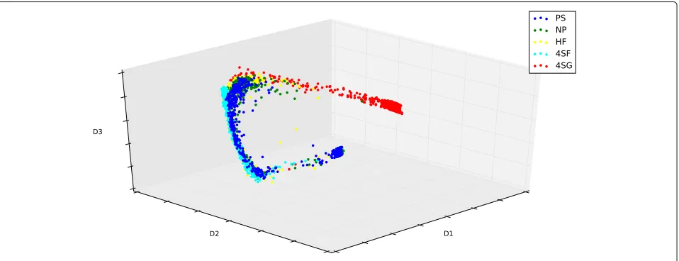
Using the single cell data, a Diffusion Map algorithm is first employed to visualize the dataset [31]. The purpose of this step is to reduce the dimension of dataset and provide the pattern of the data in the three-dimensional space. Generally we choose three eigenvectors of the ker-nel matrix (2) for visualization. These three eigenvectors are those that have the largest eigenvalues. Figure 1 gives
the diffusion coordinates for the first, second and third largest eigenvalues. It shows that all the data points in the development trajectory form only one branch. This result shows that the single cell dataset is appropriate for generating a pseudo-temporal trajectory by using the Wanderlust algorithm. This analysis also provides a single cell that will be used the first cell in the development of the pseudo-temporal trajectory.
Wanderlust ordering
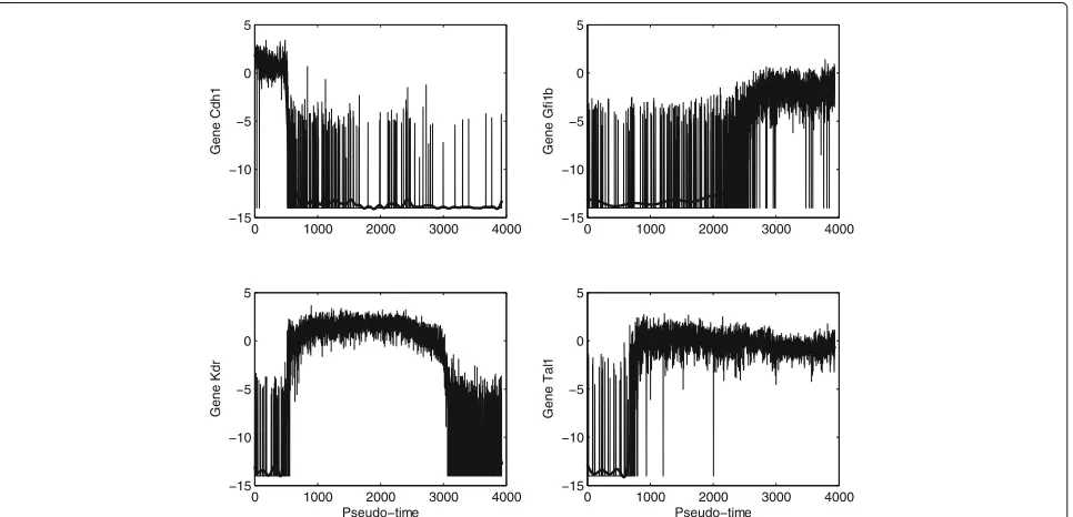
After determining the starting cell s in the previous section, the Wanderlust algorithm is then employed to obtain the pseudo-temporal trajectory for the expres-sion dynamics of genes. In this program, the widely used Euclidean measure is used to calculate the distance between different cells. Figure 2 provides the determined pseudo-temporal trajectory of four genes based on the raw dCt data in [31]. Based on the generated pseudo-temporal trajectory, we find that the expression levels of the four housekeeping genes are barely changed. Similar observa-tions can also be applied to the expression levels of genes HoxB2andHoxD8. Therefore we will not consider these six genes in the network development.
The pseudo-temporal trajectory has large variations in the expression levels of every gene. Thus it is very diffi-cult to use differential equation model to realize such data with large variation. To address issue, the Gauss process regression method is used to remove the variations in the data and produce more smooth trajectory. Figure 2 also provides the pseudo-temporal trajectory after the smooth process for the four genes. Compared with the raw dCt
data with large variations, the smoothed data for the same gene have much smaller fluctuations in the expression levels.
One characteristics of the expression levels is that all genes (excluding the six genes) have both high and low expression levels. Genetic switching exists in the expres-sion levels. Based on the time interval with high or low expression levels, the processed data can be classified into a number of patterns. For example, geneCdh1has high expression levels in the pseudo-time interval [0, 500] and low expression levels in the following time interval. How-ever, genesGfi1bandTal1have low expression level in the pseudo-time interval [0, 2500] and [0, 800], respectively, but the expression level is switched to high levels in the following time intervals. A few of genes, such as gene Kdrin Fig. 2, have two genetic switchings in the pseudo-temporal trajectory. Since our proposed technique has been used to realize the similar observations for genetic switching [45], this modelling approach will be used in this work to realized the pseudo-temporal trajectories.
Networks construction
With the availability of pseudo-temporal trajectory based on single-cell data, we then reverse-engineer the network structure for the regulatory network of 40 genes. The GENIE3 algorithm is used to develop a graphic model of these 40 genes. For each gene, a linear regression model is used to infer the regulation of other 39 genes to the expression of that gene. Then we can obtain 39 weight val-ues for the possible regulation strength for each gene and the total number of genetic regulation strength is 1560
0 1000 2000 3000 4000
−15 −10 −5 0 5
Gene Cdh1
0 1000 2000 3000 4000
−15 −10 −5 0 5
Gene Gfi1
b
0 1000 2000 3000 4000
−15 −10 −5 0 5
Gene Kdr
Pseudo−time
0 1000 2000 3000 4000
−15 −10 −5 0 5
Gene Tal
1
Pseudo−time
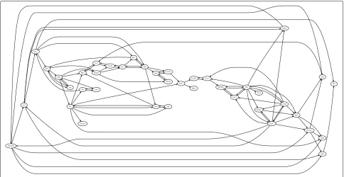
(=39×40). In order to maintain a certain number of regu-lations to each gene, we select the top 10 weight values for each gene. In this way the number of selected regulation values is only 400. Since a network with 400 undirected edges is still very dense, we set up a threshold value to select the top regulation strength. An edge is selected if its weight is larger than the threshold value. We have tested different values of the threshold value by decrease the threshold value gradually. The optimal threshold value is determined if the number of remaining edges is relative small but all genes should be connected to the network. The constructed network is given in Fig. 3. In this net-work there are 100 regulatory connections between these 40 genes. Among these 40 genes, the maximal number of connection edges for a gene is 11; while the minimal num-ber of edge for a gene is 1. The average numnum-ber of edge per gene is 2.5 and on average each gene connects to five other genes,
We have developed a mathematical model to describe the dynamics of the network with 40 genes. However, numerical results suggest that it is difficult to use a differential equation model to simulate the expression dynamics of 40 genes. The mathematical model includes a large number of model parameters that should be estimated. Due to the complexity of searching space, the simulation error is large. In addition, the genetic switch-ing in the observation data makes the designed ODE model is stiff. Therefore we consider a small network with a less number of genes. We compare the designed graphic model in Fig. 3 and the model in Figure 3C in [37], and
then select nine genes, namely GATA1, Gfi1b, Hhex,
Ikaros, Myb, Nfe2, Notch1, Sox7 andSox17. The regula-tion relaregula-tionship between these nine genes in these two networks are consistent. However, the regulation between these nine genes in our graphic model in Fig. 3 is not a fully connected network, thus the regulation between the gene pair (it Sox7, Sox17), which exists in the network in [37], was added to Fig. 4 in order to form a complete network. The developed network model is presented in Fig. 4.
Mathematical model
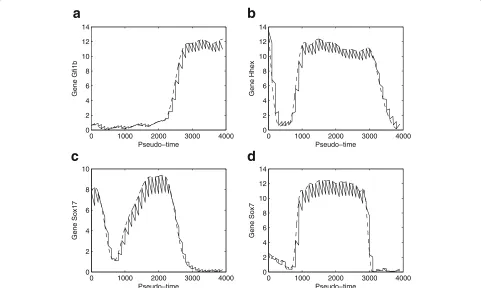
The nine genes selected in Fig. 4 is divided into two groups based on their expression patterns. In these nine genes, there are five genes, namelyGATA1, Gfi1b, Ikaros, Myb, Nfe2, whose expression are activated at the pseudo-time point t =∼ 2300 and their expression activities are promoted a high level with different speeds for dif-ferent genes. However, the expression of the remaining four genes, namelyHhex, Notch1, Sox7 and Sox17, is first inhibited and their expression levels go down to a low level at he pseudo-time pointt=∼700; but their expres-sion is activated att=∼2500 and the expressions return to the high levels again. The observed gene expression changes are consistent with other experimental observa-tions showing that genesGATA1, Gfi1bandIkarosdo have substantial changes of the expression levels over time [45]. The genetic switching in the expression levels of these genes is important to maintain the functional activities of blood stem cells. Using the proposed modelling method
Fig. 4Graphic model for the regulatory network with nine genes. All the regulations (except that for gene pairs Sox7 and Sox17) are derived from the network in Fig. 3
in [45], it is assumed that some key model parameters are variables of time rather than a constant. For the five genes in the first group, we use the following synthesis rate for gene expression, given by
ki =
ki0, t<2500 ki0∗Ai else
where ki0 is the basal synthesis rate of gene i, and Ai > 1. Regarding the four genes in the second group,
it is assumed that both synthesis rate and degrada-tion rate are variables of time, since we need to real-ize the first switching from high expression level to low expression level,
ki=
ki0∗Ai, 500<t<1000 ki0 else
di=
di0∗Ai, 2500<t<3000 di0 else
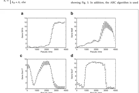
Our simulation results suggest that the proposed ODE system is still even when an implicit method with very good stability property is used for numerical solution of the proposed model. Numerical simulation will break down if we try to find the solution over a relatively long pseudo-time interval. Therefore we have to separate the whole time interval into a number of subintervals, and in each subinterval, we use the experimental observa-tion data as the initial condiobserva-tion to generate soluobserva-tion of the subinterval. Figure 5 shows simulation results using a fixed time period of 100 unit time. We have also exam-ined other lengths of time period, namely t = 50 and t = 200. Numerical results are consistent with those showing Fig. 5. In addition, the ABC algorithm is used
0 1000 2000 3000 4000
0 2 4 6 8 10 12 14
Pseudo−time
Gene Gfi1b
a
0 1000 2000 3000 4000
0 2 4 6 8 10 12 14
Pseudo−time
Gene MyB
b
0 1000 2000 3000 4000
0 2 4 6 8 10
Pseudo−time
Gene Sox17
c
0 1000 2000 3000 4000
0 2 4 6 8 10 12 14
Pseudo−time
Gene Sox7
d
to infer the unknown model parameters using the data shown in Fig. 2. Figure 5 suggests that the proposed model is able to match experimental data very well. Certainly the simulation error is dependent on the length of subinterval. The simulation error is larger if the length of subinterval is larger.
Inference of network with more regulations
The proposed network in Fig. 4 includes nine one-way or mutual regulations. It is fully consistent with the net-work predicted in [37]. To make predictions about the potential regulations among these nine genes, we extend the network by including more regulations. We apply the GENIE3 algorithm to the raw dCt data of these nine genes only. According to the calculated weight of the target edges, we select the highest weight of 27 one-way reg-ulations. Since there are a few two-way regulations in the selected 27 regulation edges, the generated network includes 17 un-directional regulations (see Additional file 1). Compared with the network in Fig. 4, the num-ber of potential regulation edges has been doubled. The structure of the extended network is shown in Additional file 1: Figure S1 in Supplementary Information. Note that the regulations in Additional file 1: Figure S1 do not include all the regulations in Fig. 4. The added regulation
(Sox 7, Sox 17) in Fig. 4 does not appear in Additional file 1: Figure S1. However, the other eight regulations in Fig. 4 also appears in Additional file 1: Figure S1.
For this extended network, we also use the ABC algo-rithm to infer model parameters using the modified dCT values. Simulation results of four genes are presented in the Fig. 6. Numerical results for the total simulation error suggest that the extended network (see Fig. 7b, index 1) has better accuracy than the network in Fig. 4 (Fig. 7a, index 1). Note that the model based on a network with more regulations has more model parameters, which gives more flexibility to match the experimental data. Thus it is reasonable that the model based on network in Additional file 1: Figure S1 has better accuracy than that in Fig. 4. However, this simulation result suggests that, compared with the network in Fig. 4, more regulations may exist.
Inference of network with auto-regulation
In the graphic model generated by the GENIE3 algorithm, the auto-regulation, namely the positive or negative regu-lation of a gene to the expression of itself, is not consid-ered. To find the potential auto-regulations in these genes, we test the network by adding positive auto-regulation to a particular gene. For thei-th gene, we setbii > 0; and
the value of aii is aii > 0 for positive auto-regulation.
0 1000 2000 3000 4000
0 2 4 6 8 10 12 14
Pseudo−time
Gene Gfi1b
0 1000 2000 3000 4000
0 2 4 6 8 10 12 14
Pseudo−time
Gene Hhex
0 1000 2000 3000 4000
0 2 4 6 8 10
Pseudo−time
Gene Sox17
0 1000 2000 3000 4000
0 2 4 6 8 10 12 14
Pseudo−time
Gene Sox7
a
b
c
d
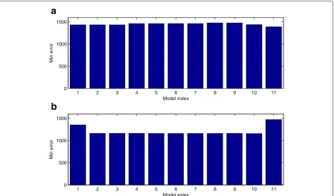
We first test the gene network shown in Fig. 4 with posi-tive auto-regulation for only one gene. Numerical results in Fig. 7a suggest that no module with positive auto-regulation (model index 2∼10) has smaller simulation error than that of the network without any auto-regulation (index 1 in Fig. 7a). We have also tested the network in which each gene has positive auto-regulation. Results in (index 11 in Fig. 7a) shows that simulation error of this module is larger than that of any other module in Fig. 7a. Thus it is unlikely that all these genes have positive auto-regulation.
We have also conducted the positive auto-regulation test for the model based on the network in Additional file 1: Figure S1. An interesting result is that, compared with the network without auto-regulation (index 1 in Fig. 7b), the model with positive auto-regulation to any one gene (model index 2∼10) has better accuracy than the network model without auto-regulation. Note that, com-pared with the network model without auto-regulation, the network model with positive auto-regulation to one gene has only two additional model parameters. The small change in the number of unknown parameters would not bring much flexibility to match experimental data. Thus this result suggests that there may be positive
auto-regulation for some genes in this network. However, when we add auto-regulation to all genes (index 11 in Fig. 7b), similar to the result in (index 11 in Fig. 7a), the simulation error of this module is larger than any other module. This gives further evidence that it is unlikely that all these genes have positive auto-regulation.
Robustness analysis
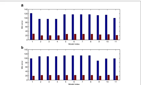
We also test the robustness property of the developed models and the models with positive auto-regulations . We first use the estimated optimal parameter set to gen-erate one simulation which is regarded as the exact simu-lation of the model without any perturbation. Then all the model parameters are perturbed by using a uniformly dis-tributed random variable, and perturbed simulations are obtained using the perturbed model parameters. We gen-erate 1000 sets of perturbed simulations and calculate the mean and variance of the simulation error for the per-turbed simulation over the unperper-turbed simulations. For the gene network shown in Figs. 4 and 8a suggests that the models with auto-regulation for genesGata1, Gfi1b, Hhex have better robustness property than the model without any perturbation. However, for the gene network with 17 regulations in Additional file 1: Figure S1, the networks
1 2 3 4 5 6 7 8 9 10 11
0 500 1000 1500
Model index
Min error
1 2 3 4 5 6 7 8 9 10 11
0 500 1000 1500
Model index
Min error
a
b
1 2 3 4 5 6 7 8 9 10 11 0
20 40 60 80 100 120 140
Model index
Min error
1 2 3 4 5 6 7 8 9 10 11
0 20 40 60 80 100 120 140
Model index
Min error
a
b
Fig. 8Robustness property of various models for the gene network with nine genes.aRobustness for the gene network in Fig. 4.bRobustness for the gene network with 17 regulations (Model index: 1: netwok without any auto-regulation, 2:10: positive auth-regulation for geneGata1, Gfi1b, Hhex, Ikaros, Myb, Nfe2, Notch1, Sox17, Sox7, respectively, 11: all nine genes have positive auto-regulation). For each model, the first bar is the mean of error; while the second bar is the variance of error
with auto-regulation for genes Sox7, Sox17 have better robustness property than the network without positive auto-regulation. These simulation results do not provide strong evidence to support the positive auto-regulation in the nine genes in Fig. 4.
Conclusion
In this work we have designed an integrated approach to reverse-engineer gene networks for regulating early blood development based on singel-cell experimental observa-tions. The diffusion map method is firstly used to obtain the visualization of gene expression data derived from 3934 stem blood cells. The wanderlust algorithm is then employed to develop the pseudo-trajectory for the activi-ties of a number of genes. Since the gene expression levels in the developed pseudo-trajectory show large fluctua-tions, we then use Gaussian process regression method to smooth the gene express data in order to obtain pseudo-trajectory with much less fluctuations. The proposed inte-grated framework consist of both the GENIE3 algorithm to reconstruct the regulatory network and a mathemat-ical model using differential equations to describe the dynamics of gene expression. The developed approach is applied to study the network regulating early blood
cell development, and we designed a graphic model for a regulatory network with forty genes and a differential equations model for a network of nine genes. The research results in this work shows that the developed approach is an efficient and effective method to reverse-engineer gene networks using single-cell experimental observations.
In this work we use simulation error as the key criterion to select the model parameters and infer the regulation between genes. However, because of the complex search-ing space of model parameters and noise in experimental data, it may be difficult to judge which model is really bet-ter than others if the difference between simulation errors is small. In fact, simulation errors of various models for the network of nine genes are quite close to each other. There-fore, in addition to using simulation error as the unique criterion to select a model, other measurements, such as AIC value, parameter identifiability and robustness prop-erty of a network, are also needed as important criteria. All of these issues are potential topics for future research.
Additional file
Acknowledgements
This research work is supported by the National Natural Science Foundation of China (11571368), and Australian Research Council Discovery Project (DP120104460).
Funding
T.T. is supported by the Australian Research Council (ARC) Discovery Projects (DP120104460) which supports the publication cost of this paper.
Availability of data and materials
Not applicable.
About this supplement
This article has been published as part ofBMC Medical GenomicsVolume 10 Supplement 5, 2017: Selected articles from the IEEE BIBM International Conference on Bioinformatics & Biomedicine (BIBM) 2016: medical genomics. The full contents of the supplement are available online at https:// bmcmedgenomics.biomedcentral.com/articles/supplements/volume-10-supplement-5.
Software
Not applicable.
Authors’ contributions
TT conceived the research. JW and TT conducted the research. JW, XH, XZ and TT interpreted the results and wrote the paper. All authors edited and approved the final version of the manuscript.
Ethics approval and consent to participate
Not applicable.
Consent to publication
Not applicable.
Competing interests
The authors declare that they have no competing interests.
Publisher’s Note
Springer Nature remains neutral with regard to jurisdictional claims in published maps and institutional affiliations.
Author details
1School of Statistics and Mathematics, Zhongnan University of Economics and Law, 430073 Wuhan, China.2School of Computer, Central China Normal University, 430079 Wuhan, China.3School of Mathematics and Statistics, Wuhan University, 430072 Wuhan, China.4School of Mathematical Sciences, Monash University, Melbourne VIC 3800, Australia.
Published: 28 December 2017
References
1. Taniguchi Y, Choi PJ, Li GW, Chen H, Babu M, Hearn J, Emili A, Xie XS. Quantifying E. coli proteome and transcriptome with single-molecule sensitivity in single cells. Science. 2010;329:533–8.
2. Dumitriu A, Golji J, Labadorf AT, Gao B, Beach TG, Myers RH, Longo KA, Latourelle JC. Integrative analyses of proteomics and RNA transcriptomics implicate mitochondrial processes, protein folding pathways and GWAS loci in Parkinson disease. BMC Med Genomics. 2016;9:5.
3. Munsky B, Neuert G, van Oudenaarden A. Using gene expression noise to understand gene regulation. Science. 2012;336:183–7.
4. Espinosa Angarica V, Del Sol A. Modeling heterogeneity in the pluripotent state: A promising strategy for improving the efficiency and fidelity of stem cell differentiation. Bioessays. 2016;38:758–68.
5. Waldron D. Gene expression: Environmental noise control. Nat Rev Genet. 2015;16:624–5.
6. Junker JP, van Oudenaarden A. Every cell is special: genome-wide studies add a new dimension to single-cell biology. Cell. 2014;157:8–11. 7. Deng Q, Ramskold D, Reinius B, Sandberg R. Single-cell RNA-seq reveals
dynamic, random monoallelic gene expression in mammalian cells. Science. 2014;343:193–6.
8. Wei W, Shin YS, Ma C, Wang J, Elitas M, Fan R, Heath JR. Microchip platforms for multiplex single-cell functional proteomics with applications to immunology and cancer research. Genome Med. 2013;5:75.
9. Buganim Y, Faddah D, Cheng A, Itskovich E, Markoulaki S, Ganz K, Klemm S, Vanoudenaarden A, Jaenisch R. Single-cell expression analyses during cellular reprogramming reveal an early stochastic and a late hierarchic phase. Cell. 2012;150(6):1209–22.
10. Stegle O, Teichmann SA, Marioni JC. Computational and analytical challenges in single-cell transcriptomics. Nat Rev Genet. 2015;16:133–45. 11. Poirion OB, Zhu X, Ching T, Garmire L. Single-Cell Transcriptomics
Bioinformatics and Computational Challenges. Front Genet. 2016;7:163. 12. Woodhouse S, Moignard V, Göttgens B, Fisher J. Processing, visualising and reconstructing network models from single-cell data. Immunol Cell Biol. 2015;94:256–65.
13. Marr C, Zhou JX, Huang S. Single-cell gene expression profiling and cell state dynamics: collecting data, correlating data points and connecting the dots. Curr Opin Biotechnol. 2016;39:207–14.
14. Moignard V, Macaulay IC, Swiers G, Buettner F, Schütte J, Calero-Nieto FJ, et al. Characterization of transcriptional networks in blood stem and progenitor cells using high-throughput single-cell gene expression analysis. Nat Cell Biol. 2013;15:363–72.
15. Bendall SC, Davis KL, Amir el-AD, Tadmor MD, Simonds EF, Chen TJ, Shenfeld DK, Nolan GP, Pe’er D. Single-cell trajectory detection uncovers progression and regulatory coordination in human b cell development. Cell. 2014;157(3):714–25.
16. Penfold CA, Wild DL. How to infer gene networks from expression profiles, revisited. Interface Focus. 2011;1:857–70.
17. Bar-Joseph Z, Gitter A, Simon I. Studying and modelling dynamic biological processes using time-series gene expression data. Nat Rev Genet. 2012;13:552–64.
18. Maetschke SR, Madhamshettiwar PB, Davis MJ, Ragan MA. Supervised, semi-supervised and unsupervised inference of gene regulatory networks. Brief Bioinform. 2012;15:195–211.
19. Wang J, Cheung LW, Delabie J. New probabilistic graphical models for genetic regulatory networks studies. J Biomed Inform. 2005;38:443–55. 20. Sachs K, Perez O, Pe’Er D, Lauffenburger DA, Nolan GP. Causal
protein-signaling networks derived from multiparameter single-cell data. Science. 2005;308:523–9.
21. Brown MPS, Grundy WN, Lin D, Cristianini N, Sugnet CW, Furey TS, Ares M, Haussler D. Knowledge-based analysis of microarray gene expression data by using support vector machines. Proc Natl Acad Sci. 2000;97:262–7. 22. Kim Y, Han S, Choi S, Hwang D. Inference of dynamic networks using
time-course data. Brief Bioinformatics. 2014;15:212–28.
23. Chasman D, Siahpirani AF, Roy S. Network-based approaches for analysis of complex biological systems. Curr Opin Biotechnol. 2016;39:157–66. 24. Wang J, Tian T. Quantitative model for inferring dynamic regulation of
the tumour suppressor gene p53. BMC Bioinformatics. 2010;11(1):36. 25. Ocone A, Sanguinetti G. Reconstructing transcription factor activities in
hierarchical transcription network motifs. Bioinformatics. 2011;27:2873–9. 26. Maraziotis IA, Dragomir A, Thanos D. Gene regulatory networks modelling
using a dynamic evolutionary hybrid. BMC Bioinformatics. 2010;11(1):1. 27. Petralia F, Wang P, Yang J, Tu Z. Integrative random forest for gene
regulatory network inference. Bioinformatics. 2015;31(12):i197–i205. 28. Marbach D, Costello JC, Küffner R, Vega NM, Prill RJ, Camacho DM,
Allison KR, Kellis M, Collins JJ, Stolovitzky G. Wisdom of crowds for robust gene network inference. Nat Methods. 2012;9:796–804.
29. Kim D, Kang M, Biswas A, Liu C, Gao J. Integrative approach for inference of gene regulatory networks using lasso-based random featuring and application to psychiatric disorders. BMC Med Genomics. 2016;9(Suppl 2):50.
30. Wang J, Wu Q, Hu X, Tian T. An integrated approach to infer dynamic protein-gene interactions – a case study of the human p53 protein. Methods. 2016;110:3–13.
31. Ocone A, Haghverdi L, Mueller NS, Theis FJ. Reconstructing gene regulatory dynamics from high-dimensional single-cell snapshot data. Bioinformatics. 2015;31:i89–i96.
33. Ji Z, Ji H. Tscan: Pseudo-time reconstruction and evaluation in single-cell RNA-seq analysis. Nucleic Acids Res. 2016;44:e177.
34. Pina C, Teles J, Fugazza C, May G, Wang D, Guo Y, Soneji S, Brown J, Edén P, Ohlsson M. Single-cell network analysis identifies ddit3 as a nodal lineage regulator in hematopoiesis. Cell Reports. 2015;24:1503–10. 35. Trapnell C, Cacchiarelli D, Grimsby J, Pokharel P, Li S, Morse M,
Lennon NJ, Livak KJ, Mikk elsen TS, Rinn JL. Pseudo-temporal ordering of individual cells reveals dynamics and regulators of cell fate decisions. Nat Biotechnol. 2014;32:381.
36. Haghverdi L, Buettner F, Theis FJ. Diffusion maps for high-dimensional single-cell analysis of differentiation data. Bioinformatics. 2015;31(18): 2989–98.
37. Moignard V, Woodhouse S, Haghverdi L, Lilly AJ, Tanaka Y, Wilkinson AC, Buettner F, Macaulay IC, Jawaid W, Diamanti E, et al. Decoding the regulatory network of early blood development from single-cell gene expression measurements. Nat biotechnol. 2015;33:269–76. 38. Williams CKI, Rasmussen CE. Gaussian processes for machine learning.
Cambridge: MIT Press; 2006, pp. 7–32.
39. Irrthum A, Wehenkel L, Geurts P, et al. Inferring regulatory networks from expression data using tree-based methods. PloS ONE. 2010;5(9):e12776. 40. Huynh-Thu VA, Irrthum A, Wehenkel L, Geurts P. Inferring regulatory
networks from expression data using tree-based methods. Plos ONE. 2009;5(9):e12776.
41. Shea MA, Ackers GK. The OR control system of bacteriophage lambda. A physical-chemical model for gene regulation. J Mol Biol. 1985;181(2): 211–30.
42. Turner BM, Van Zandt T. A tutorial on approximate Bayesian computation. J Math Psych. 2012;56:69–85.
43. Wu Q, Smith-Miles K, Tian T. Approximate bayesian computation schemes for parameter inference of discrete stochastic models using simulated likelihood density. BMC Bioinfomatics. 2014;15(S12):S3. 44. Kitano H. Towards a theory of biological robustness. Mol Syst Biol.
2007;3:137.
45. Tian T, Smith-Miles K. Mathematical modeling of gata-switching for regulating the differentiation of hematopoietic stem cell. BMC Systems Biol. 2014;8(S1):S8.
• We accept pre-submission inquiries
• Our selector tool helps you to find the most relevant journal • We provide round the clock customer support
• Convenient online submission • Thorough peer review
• Inclusion in PubMed and all major indexing services • Maximum visibility for your research
Submit your manuscript at www.biomedcentral.com/submit