Mass-conserving subglacial hydrology in the Parallel Ice Sheet Model version 0.6

www.geosci-model-dev.net/8/1613/2015/ doi:10.5194/gmd-8-1613-2015

© Author(s) 2015. CC Attribution 3.0 License.

Mass-conserving subglacial hydrology in the Parallel Ice Sheet

Model version 0.6

E. Bueler1and W. van Pelt2,*

1_{Department of Mathematics and Statistics and Geophysical Institute, University of Alaska Fairbanks, USA} 2_{Institute for Marine and Atmospheric Research Utrecht, the Netherlands}

*_{current address: Department of Earth Sciences, Uppsala University, Sweden}

Correspondence to: Ed Bueler ([email protected])

Received: 20 June 2014 – Published in Geosci. Model Dev. Discuss.: 29 July 2014 Revised: 22 April 2015 – Accepted: 23 April 2015 – Published: 2 June 2015

Abstract. We describe and test a two-horizontal-dimension subglacial hydrology model which combines till with a dis-tributed system of water-filled, linked cavities which open through sliding and close through ice creep. The addition of this sub-model to the Parallel Ice Sheet Model (PISM) ac-complishes three specific goals: (a) conservation of the mass of water, (b) simulation of spatially and temporally variable basal shear stress from physical mechanisms based on a min-imal number of free parameters, and (c) convergence un-der grid refinement. The model is a common generalization of four others: (i) the undrained plastic bed model of Tu-laczyk et al. (2000b), (ii) a standard “routing” model used for identifying locations of subglacial lakes, (iii) the lumped englacial–subglacial model of Bartholomaus et al. (2011), and (iv) the elliptic-pressure-equation model of Schoof et al. (2012). We preserve physical bounds on the pressure. In steady state a functional relationship between water amount and pressure emerges. We construct an exact solution of the coupled, steady equations and use it for verification of our ex-plicit time stepping, parallel numerical implementation. We demonstrate the model at scale by 5 year simulations of the entire Greenland ice sheet at 2 km horizontal resolution, with one million nodes in the hydrology grid.

1 Introduction

Any continuum-physics-based dynamical model of the liq-uid water underneath and within a glacier or ice sheet has at least these two elements: the mass of the water is conserved and the water flows from high to low values of the

mod-eled hydraulic potential. Beyond that there are many varia-tions considered in the literature. Modeled aquifer geometry might be a system of linked cavities (Kamb, 1987), conduits (Nye, 1976), or a sheet (Creyts and Schoof, 2009). Geome-try evolution processes might include the opening of cavities by sliding of the overlying ice past bedrock bumps (Schoof, 2005), the creation of cavities by interaction of the ice with deformable sediment (Schoof, 2007), closure of cavities and conduits by creep (Hewitt, 2011), or melt on the walls of cavities and conduits which causes them to open (Clarke, 2005). Water could move in a macro-porous englacial sys-tem (Bartholomaus et al., 2011) or it could be stored in a porous till (Tulaczyk et al., 2000a).

Models have combined subsets of these different mor-phologies and processes (Flowers and Clarke, 2002a; He-witt, 2013; Hoffman and Price, 2014; Van der Wel et al., 2013; Werder et al., 2013; de Fleurian et al., 2014). However, the completeness of the modeled processes must be balanced against the number of uncertain model parameters and the ultimate availability of observations with which to constrain them.

This paper describes a carefully selected model for a dis-tributed system of linked subglacial cavities, with additional storage of water in the pore spaces of subglacial till. Water in excess of the capacity of the till passes into the distributed transport system. In this sense the model could be called a “drained-and-conserved” extension of the “undrained” plas-tic bed model of Tulaczyk et al. (2000b).

the relationship between water amount and pressure. Pres-sure is thereby determined non-locally over each connected component of the hydrological system. No functional rela-tion between subglacial water amount and pressure is as-sumed (compare Flowers and Clarke, 2002a). The pressure solves an equation which is a parabolic regularization of the distributed pressure equation given in elliptic variational in-equality form by Schoof et al. (2012).

In cases where boreholes have actually been drilled to the ice base, till is often observed (Hooke et al., 1997; Tu-laczyk et al., 2000a; Truffer et al., 2000; Truffer and Harri-son, 2006). Laboratory experiments on the rheology of till (Kamb, 1991; Hooke et al., 1997; Tulaczyk et al., 2000a; Truffer et al., 2001) generally conclude that its deformation is well approximated by a Mohr–Coulomb relation (Schoof, 2006b). For this reason we adopt a compressible-Coulomb-plastic till model when determining the effective pressure on the till as a function of the amount of water stored in it (Tu-laczyk et al., 2000a). Existing models which combine till and a mass-conservation equation for the subglacial water are rather different from ours, as they either have only one-horizontal dimension (Van der Wel et al., 2013) or have a pressure equation which directly ties water pressure to wa-ter amount, which generates a porous-medium equation form (Flowers and Clarke, 2002a; de Fleurian et al., 2014).

The major goals here are to implement, verify, and demon-strate this two-dimensional subglacial hydrology model. The model is applicable at a wide variety of spatial and tempo-ral scales but it has relatively few parameters. It is patempo-ral- paral-lelized and it exhibits convergence of solutions under grid refinement. It is a sub-model of a comprehensive three-dimensional ice sheet model, the open-source Parallel Ice Sheet Model (PISM; http://pism-docs.org); the sub-model can be added to any PISM run by a simple run-time option.

Channelized subglacial flow is widely assumed to occur in Greenland, based on borehole and moulin evidence (An-drews et al., 2014, for example). This important physical pro-cess for subglacial hydrologic transport is not captured by our model because conduits are not modeled. Existing theo-ries of conduits apparently require their locations to be fixed a priori (Schoof, 2010b; Hewitt, 2013; Werder et al., 2013). Such lattice models have no known continuum limit in the map plane. By contrast with conduits, linked-cavity models do not put the cavities at the nodes of a pre-determined lat-tice, exactly because the continuum limit of such a lattice model is known (Hewitt, 2011), namely as a partial differen-tial equation (PDE; Eq. 13 in the current paper). Regarding lattice models, because all PISM usage involves a run-time determination of grid resolution, all parameters must have grid-spacing-independent meaning. Lattice or other input-grid-based models are therefore not acceptable as compo-nents of PISM.

Wall melt in the linked-cavity system, which is believed to be small (Kamb, 1987), is not added into the mass-conservation equation in our model. (It can be calculated

diagnostically from the modeled flux and hydraulic gradi-ent, however.) If included in mass conservation, the addi-tion of wall melt can generate an unstable distributed system (Walder, 1982), though such a system can be stabilized to some degree by bedrock bumps (Creyts and Schoof, 2009).

The structure of the paper is as follows: Sect. 2 consid-ers basic physical principles, culminating with a fundamen-tal advection–diffusion form of the mass-conservation equa-tion. Section 3 reviews what is known about till mechanical properties, water in till pore spaces, and shear stress at the base of a glacier. In Sect. 4 we compare “closures” which di-rectly or indidi-rectly determine the subglacial water pressure. Based on all these elements, in Sect. 5 we summarize the new model and the role of its major fields. In this section we show how the model extends several published models, we note properties of its steady states (see also Appendix A), and we compute a nearly exact steady solution in the map plane, a useful tool for verification. In Sect. 6 we present the numerical schemes, with particular attention to time-step re-strictions and the treatment of advection, and we document the PISM options and parameters seen by users. Section 7 shows numerical results from the model, starting with con-vergence under grid refinement in the verification case. We then demonstrate the model in 5 year runs on a 2 km grid covering the entire Greenland ice sheet.

2 Elements of subglacial hydrology 2.1 Mass conservation

We assume that liquid water is of constant densityρw; see Table 1 for constants. Thus, the thickness of the layer of lat-erally moving water, denoted byW (t, x, y), determines its mass; see Table 2 for variable names and meanings. In ad-dition there is liquid water stored locally in the pore spaces of till (Tulaczyk et al., 2000b) which is also described by an effective thicknessWtil(t, x, y). Such thicknesses are only meaningful compared to observations if they are regarded as averages over a horizontal scale of meters to hundreds of meters (Flowers and Clarke, 2002a). Thus, the total effec-tive thickness of the water at map-plane location(x, y) and timetisW+Wtil. This sum is the conserved quantity in our model. In two map-plane dimensions the mass-conservation equation is (compare Clarke, 2005)

∂W ∂t +

∂Wtil

∂t + ∇ ·q= m ρw

, (1)

where∇· = ∂

∂x+ ∂

∂y denotes divergence,qis the vector

wa-ter flux (m2s−1), andmis the total input to the subglacial hydrology (kg m−2s−1). Note that the water fluxq is con-centrated within the two-dimensional subglacial layer.

Table 1. Physical constants and model parameters. All values are configurable in PISM; see Table 3.

Name Default Units Description

A 3.1689×10−24 Pa−3s−1 ice softness (Huybrechts et al., 1996)

α 5₄ power in flux formula (Schoof et al., 2012)

β 3₂ power in flux formula (Schoof et al., 2012)

c0 0 Pa till cohesion (Tulaczyk et al., 2000a) c1 0.5 m−1 cavitation coefficient (Schoof et al., 2012) c2 0.04 creep closure coefficient

Cc 0.12 till compressibility (Tulaczyk et al., 2000a) Cd 0.001 m a−1 background till drainage rate

δ 0.02 Ntillower bound, as fraction of overburden pressure e0 0.69 reference void ratio atN0(Tulaczyk et al., 2000a) φ0 0.01 notional (regularizing) englacial porosity g 9.81 m s−2 acceleration of gravity

k 0.001 m2β−αs2β−3kg1−β conductivity coefficient (Schoof et al., 2012)

N0 1000 Pa reference effective pressure (Tulaczyk et al., 2000a) ρi 910 kg m−3 ice density (Greve and Blatter, 2009)

ρw 1000 kg m−3 fresh water density (Greve and Blatter, 2009)

Wr 0.1 m roughness scale (Hewitt et al., 2012)

W_tilmax 2 m maximum water in till (Bueler and Brown, 2009)

Table 2. Functions used in the subglacial hydrology model (Eq. 32).

Type Description (symbol, units, meaning)

State

W m transportable water thickness

Wtil m till-stored water thickness P Pa transportable water pressure

Input

b m bedrock elevation

ϕ till friction angle

H m ice thickness

m kg m−2s−1 total melt water input

|vb| m s−1 ice sliding speed

Output Ntil Pa till effective pressure

τc Pa till yield stress

such as Antarctica and the interior of Greenland, the basal melt rate part of mis dominated by the energy balance at the base of the ice (Aschwanden et al., 2012). The Greenland results in Sect. 7 use only that basal melt for m. Drainage from the surface has also been added tomin applications of our model (Van Pelt, 2013), but modeling such drainage is outside the scope of this paper.

2.2 Hydraulic potential and water pressure

The hydraulic potential ψ (t, x, y) combines the pressure P (t, x, y)of the transportable subglacial water and the grav-itational potential of the top of the water layer (Goeller et al., 2013; Hewitt et al., 2012),

ψ=P+ρwg (b+W ). (2)

Herez=b(x, y)is the bedrock elevation.

We have added the term “ρwgW” to the standard hydraulic potential formula ψ=P+ρwgb (Clarke, 2005; Shreve, 1972) because differences in the potential at the top of the subglacial water layer determine the driving potential gradi-ent for a fluid layer. When the water depth becomes substan-tial (W1 m), as it would be in a subglacial lake, this term keeps the modeled lakes from being singularities of the water thickness field (compare Le Brocq et al., 2009).

Ice is a viscous fluid which has a stress field of its own. The basal value of the downward normal stress, called the overburden pressure, is denoted byPo. We accept the shal-low approximation that this stress is hydrostatic (Greve and Blatter, 2009):

Po=ρigH, (3)

whereHis the ice thickness.

OverpressureP > Pohas been observed in ice sheets, but only for short durations (Das et al., 2008). In our model and others (Schoof et al., 2012), however, because the condition P > Pois presumed to cause the ice to lift and thus reduce the pressure back to overburdenP =Po, the pressure solu-tion is subject to inequalities

0≤P ≤Po. (4)

2.3 Darcy flow

Subglacial water flows from high to low hydraulic potential. The simplest expression of this is a Darcy flux model for a water sheet:

where the hydraulic conductivity K is a constant (Clarke, 2005). More generally Schoof et al. (2012) suggests a power-law form

q= −k Wα|∇ψ|β−2∇ψ (6) forα≥1,β >1, and a coefficientk >0 with units that de-pend onαandβ(see Table 1). Clarke (2005) suggestsα=1 andβ=2, to give Eq. (5) above, Creyts and Schoof (2009) use α=3/2 andβ=3/2, Hewitt (2011, 2013) usesα=3 and β=2, and Hewitt et al. (2012) suggest α=5/4 and β=3/2. The current paper generally implements Eq. (6) but uses the Clarke (2005) and Hewitt et al. (2012) exponents in an exact solution and in numerical experiments, respec-tively. We callK=k Wα−1|∇ψ|β−2the effective hydraulic conductivity, so that Eq. (5) applies formally throughout. 2.4 Advection–diffusion decomposition

Combining Eqs. (2) and (6), and separating the term propor-tional to∇W, we get the flux expression

q= −kWα|∇ψ|β−2∇(P+ρwgb) (7) −ρwgkWα|∇ψ|β−2∇W,

which suggests a mix of mechanisms. If P scales with the overburden pressurePo, and if|∇(H+b)| |∇W|, then the first flux term in Eq. (7) will dominate. In any case, the sec-ond term with∇W acts diffusively in the mass conservation Eq. (1). We will see that in near-steady-state circumstances where there is significant sliding, the first term with ∇P is also significantly diffusive in the mass-conservation equation (Sect. 5.3). In conditions far from steady state, however, the direction of∇P is presumably different from the direction ∇W.

We will construct our numerical scheme based on decom-position Eq. (7). To simplify the expression slightly, the small thickness approximationW≈0 is made inside the absolute value signs in Eq. (7), namely,

|∇ψ| ≈ |∇(P+ρwgb)|. (8) This simplification, which makes no change in theβ=2 case (see Sect. 2.3), lets us redefine the effective hydraulic con-ductivity as

K=kWα−1|∇(P+ρwgb)|β−2. (9)

In terms of K we define a velocity field and a diffusivity coefficient:

V = −K∇(P+ρwgb) , D=ρwgKW, (10)

so that Eq. (7) is a clean advection–diffusion decomposition:

q=VW−D∇W. (11)

From Eqs. (1) and (11) we now have an advection– diffusion-production equation for the evolution of the con-served water amountW+Wt il:

∂W ∂t +

∂Wtil

∂t = −∇ ·(VW )+ ∇ ·(D∇W )+ m ρw

. (12)

There are distinct numerical approximations for the advec-tion term∇ ·(VW )and the diffusion term∇ ·(D∇W ), with time-step restrictions of different magnitudes (Sect. 6). Equa-tion (12) is often advecEqua-tion dominated in the sense that |VW| |D∇W|, and numerical schemes for advection and diffusion must be tested in combination (Sect. 7).

2.5 Capacity of a linked-cavity distributed system The rate of change of the area-averaged thickness of the cav-ities in a distributed linked-cavity system is the difference of opening and closing rates (Hewitt, 2011). This thicknessY, also called “bed separation” (Bartholomaus et al., 2011), has the generic evolution equation

∂Y

∂t =O(|vb|, Y )−C(N, Y ), (13)

wherevbis the ice base (sliding) velocity andN=Po−P is the effective pressure on the cavity system. DenotingX+= max{0, X}, we choose a non-negative opening term based on cavitation only:

O(|vb|, Y )=c1|vb|(Wr−Y )+. (14) Herec1is a scaling coefficient andWris a maximum rough-ness scale of the basal topography (Schoof et al., 2012); see Table 1. The closing term models ice creep only (Hewitt, 2011; Schoof et al., 2012):

C(N, Y )=c2AN3Y, (15)

wherec2 is a scaling coefficient and A is the softness of the ice. We have used Glen exponent n=3 for concrete-ness and simplicity. The closing termC in Eq. (15) is non-negative because our modeled pressureP satisfies the bounds 0≤P ≤Po.

3 Till hydrology and mechanics

Till with pressurized liquid water in its pore spaces is ex-pected to support much of the ice overburden. When present, such saturated till is central to the complicated relationship between the amount of subglacial water and the speed of sliding. Our model includes storage of subglacial water in till both because of its role in conserving the mass of liquid water and its role in determining basal shear stress.

in the till are regarded as filled with ice and the basal shear stress is correspondingly high. WhenWtilattains sufficiently large values, however, the till is regarded as saturated with liquid, and a drop in effective pressure becomes possible (Sect. 3.2 below).

3.1 Evolution of till-stored water layer thickness The water in till pore spaces is much less mobile than that in the linked-cavity system because of the very low hydraulic conductivity of till (Lingle and Brown, 1987; Truffer et al., 2001). Therefore, we choose an evolution equation for Wtil without horizontal transport for simplicity (Tulaczyk et al., 2000a), namely,

∂Wtil

∂t =

m ρw

−Cd. (16)

HereCd≥0 is a fixed rate that makes the till gradually drain in the absence of water input; we choose Cd=1 mm a−1, which is small compared to typical values ofm/ρw. Refreeze is also allowed, as a negative value form.

As in Bueler and Brown (2009), we constrain the layer thickness by

0≤Wtil≤Wtilmax. (17)

Any water in excess of the capacity of the till, i.e., W_tilmax, “overflows” the till and enters the transport system; it is conserved. Because the source term m in Eq. (16), or the whole right side, can be negative, the lower bound in inequal-ities (17) must be actively enforced. The upper bound in in-equalities (17) also relates to the effective pressure on the till, as we explain next.

3.2 Effective pressure on the till

Deformation of saturated till is well modeled by a plastic (Coulomb friction) or nearly plastic rheology (Hooke et al., 1997; Truffer et al., 2000; Tulaczyk et al., 2000a; Schoof, 2006b). Its yield stressτcsatisfies the Mohr–Coulomb rela-tion:

τc=c0+(tanϕ)Ntil, (18)

wherec0is the till cohesion,ϕ is the till friction angle, and Ntilis the effective pressure of the overlying ice on the satu-rated till (Cuffey and Paterson, 2010). (Note that the effective pressureN=Po−P used in Sect. 2.5 for modeling cavity closure is distinct from Ntil in Eq. (18). This distinction is again explained by the very low hydraulic conductivity of till.)

Lete=Vw/Vs be the till void ratio, whereVwis the vol-ume of water in the pore spaces andVsis the volume of min-eral solids (Tulaczyk et al., 2000a). From the standard the-ory of soil mechanics and from laboratthe-ory experiments on

till (Hooke et al., 1997; Tulaczyk et al., 2000a), a linear rela-tion exists betweeneand the logarithm ofNtil,

e=e0−Cclog10(Ntil/N0) . (19)

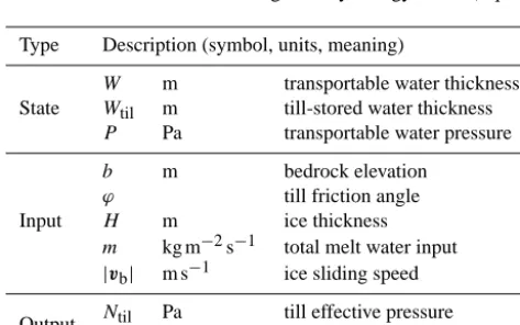
Figure 1a shows a graph of Eq. (19). Heree0is the void ratio at a reference effective pressureN0, andCcis the coefficient of compressibility of the till. Equivalently to Eq. (19),Ntil is an exponential function ofe, namely,Ntil=N010(e0−e)/Cc (Van der Wel et al., 2013, Eq. 15), soNtil is nonzero for all finite values ofe.

While Eq. (19) suggests that the effective pressure could be any positive number, in fact the area-averaged value of Ntilunder ice sheets and glaciers has limits. It cannot exceed the overburden pressure for any sustained period. Further-more, once the till is close to its maximum capacity then the excess water will be “drained” into a transport system. We suppose this occurs at a small, fixed fractionδ of the over-burden pressure. Thus, we assume the bounds

δPo≤Ntil≤Po, (20)

whereδ=0.02 in the experiments in this paper.

The void ratioe and the effective water layer thickness Wtilare describing the same thing, namely, the amount of liq-uid water in the till. In fact, if1x,1yare the horizontal di-mensions of a rectangular patch of till with (mineral-portion) thicknessηthenVw=Wtil1x 1yandVs=η 1x 1y. Thus, e=Wtil

η . (21)

On the other hand, we specify a maximumW_tilmaxon the water layer thickness, in the bounds (17). The minimumNtil=δPo of the effective pressure occurs at maximum values of void ratioeand effective thicknessWtil, so Eqs. (19) and (21) al-low us to express the solid-till thicknessη in terms of our preferred parametersW_tilmax,δ,e0,N0, andCc:

η= W

max til e0−Cclog10

δPo

N0

. (22)

From Eqs. (19), (21), and (22), the effective pressureNtil can now be written as the following function ofWtil:

ˆ Ntil=N0

_δP

o N0

s

10( e₀

Cc) (1−s)_{, (23)}

where s=Wtil/W_tilmax. However, as noted above, Ntil is bounded:

Ntil=min

n

Po,Nˆtil

o

. (24)

This function is shown in Fig. 1b.

0.0 0.1 0.2 0.3 0.4 0.5 0.6 0.7 0.8

e

0 20 40 60 80 100 120

N

(bar)

(

e

,N

)

(a)

0.0 0.5 1.0 1.5 2.0 2.5 3.0 3.5

W

(m)

20 40 60 80 100 120

N

(bar)

N

=

P

(

W

,δP

)

(b)

Figure 1. (a) Equation (19) determines the effective pressureNtilas

a function of the void ratioe; reference valuese0,N0are indicated. (b) The same curve, but withNtilas a function ofWtil, with bounds

above by overburden pressurePoand below by a fixed fractionδof

Po; the solid curve is used in our model. The case shown has 1000 meters ice thickness.

i. Experiments on till suggest small values for cohesionc0 in Eq. (18), 0≤c0.1 kPa (Tulaczyk et al., 2000a), and we choosec0=0 for concreteness.

ii. Measured till friction angles ϕ are in a 18–40◦ range (Cuffey and Paterson, 2010). Simulations of the whole Antarctic (Martin et al., 2011) and Greenlandic (As-chwanden et al., 2013) ice sheets have been based on a hypothesis that the till friction angle ϕ depends on bed elevation so as to model the submarine history of low-elevation sediments.

iii. The ratioe0/Cccan be determined by laboratory experi-ments on till samples (e.g., Hooke et al., 1997; Tulaczyk et al., 2000a). Values for the dimensionless constantse0 andCc used here (Table 1) are from till samples from ice stream B in Antarctica (Tulaczyk et al., 2000a), and they givee0/Cc=5.75 in Eq. (23).

iv. The till capacity parameter W_tilmax could be set in a location-dependent manner from in situ (Tulaczyk et al., 2000a) or seismic reflection (Rooney et al., 1987) evi-dence, but for simplicity we set it to a constant 2 m.

3.3 Sliding law

Observe that the ice sliding velocity vb is an input into the subglacial hydrology model we are building, because of Eq. (14). On the other hand, the yield stressτcis an output of the till-related part of the hydrology model (Sect. 3.2). In an ice dynamics model like PISM,vbis determined by solv-ing a stress balance in which the vector basal shear stressτb appears either as a boundary condition (Schoof, 2010a) or as a term in a vertically integrated balance (Schoof, 2006a; Bueler and Brown, 2009). In PISM,τc andvbcombine to determineτbthrough a sliding law

τb= −τc vb |vb|1−qvq₀

, (25)

where 0≤q≤1 and v0 is a threshold sliding speed (As-chwanden et al., 2013).

Power-law Eq. (25) generalizes, and includes as the case q=0, the purely plastic (Coulomb) relation τb= −τcvb/|vb|. At least in theq1 cases, under Eq. (25) the till “yields” and the magnitude of the basal shear stress be-comes nearly independent of |vb|, when |vb| v0. Equa-tion (25) could also be written in generic power-law form τb= −β|vb|q−1vbwith coefficientβ=τc/v₀q; in the linear caseq=1 we haveβ=τc/v0.

4 Closures to determine pressure

The evolution equations listed so far, namely, Eqs. (12), (13), and (16), can be simplified to three equations in the four ma-jor variablesW,Wtil,Y, andP. We do not yet know how to compute the water pressureP or its rate of change∂P /∂t given the other variables and data of the problem. A closure is needed.

4.1 Simplified closures without cavity evolution

We first consider two simple closures which appear in the literature but which do not use cavity evolution Eq. (13) or similar physics. We list them because the resulting simpli-fied conservation equations emerge as reductions of our more complete theory. For simplicity we present them without till storage (W_tilmax=0) and only in the constant conductivity case (α=1 andβ=2).

Setting the pressure equal to the overburden pressure is the simplest closure (Le Brocq et al., 2009; Shreve, 1972):

P =Po. (26)

ice-geometry-determined velocityVe,

∂W

∂t = −∇ · VeW

+ ∇ ·(ρwgk W∇W )+ m ρw

, (27)

e

V = −ρwgk

_ρ

i ρw

∇H+

1− ρi ρw

∇b

.

Because the approximation WH is usually accepted, so that the hydraulic potential is insensitive to the water layer thickness, i.e., ψ=Po+ρwgb(Le Brocq et al., 2009), the diffusion term in Eq. (27) is usually not included. With this common simplification, Eq. (27) becomes an advection equa-tion with a source term. It therefore possesses characteristic curves, trajectories of the water flow or “pathways” (Liv-ingstone et al., 2013), which are determined by ice sheet geometry. However, without the diffusion term, Eq. (27) exhibits continuum solutions with infinite water concentra-tion at every locaconcentra-tion where the simplified potential ψ= Po+ρwgbhas a minimum. Applications therefore only com-pute the characteristic curves themselves. We prefer Eq. (27) as stated, with the diffusion term, because it is well posed for positive initial and boundary values onW (compare Hewitt et al., 2012), so that numerical solutions can converge under sufficient grid refinement.

At an almost opposite extreme, our second simplified clo-sure makes the water presclo-sure a function of the amount of water. Specifically, Flowers and Clarke (2002a) proposed

PFC(W )=Po

_W

Wcrit

7₂

, (28)

where, for Trapridge glacier, Flowers and Clarke (2002b) used Wcrit=0.1 m. Thus, no separate pressure evolution equation needs to be solved.

One concern with form Eq. (28) is that PFC(W )can be arbitrarily larger than overburden pressure (Schoof et al., 2012). In any case, Eq. (28) is used in Eqs. (1) and (6) to yield a nonlinear diffusion which generalizes the porous-medium equation∂W/∂t= ∇2(Wγ)(Vázquez, 2007). The main idea in such a nonlinear diffusion is that the direction of the flux is −∇W. However, a Darcy-type modelq∼ −∇ψlike Eq. (6) normally gives flux directions different from−∇Win many cases, especially in rapidly evolving hydrologic systems, if the pressure is determined by a more physical closure. We consider such a closure next.

4.2 Full-cavity closure

Simply requiring the subglacial layer to be full of water is also a closure (Bartholomaus et al., 2011), which we adopt:

W =Y. (29)

The consequences of this closure are explored at some length by Schoof et al. (2012), Hewitt et al. (2012), and Werder et al. (2013), who describe the full-cavity case as the “normal pres-sure” condition.

Equation (29) obviously allows us to eliminate eitherWor Y as a state variable. We choose to eliminateY becauseWis already part of the conserved massW+Wtil. In the zero till storage case, Eqs. (1), (13), and (29) imply

O(|vb|, W )−C(N, W )+ ∇ ·q= m ρw

, (30)

which is exactly elliptic pressure Eq. (2.12) of Schoof et al. (2012). They argue that a model based on Eq. (30) should accommodate the possibility of partially empty cavities with W < Y whenP =0. However, like Werder et al. (2013) who implement the model in two dimensions, we accept a poten-tial loss of model completeness by using a full-cavity model. 4.3 Englacial porosity as a pressure regularization Englacial systems of cracks, crevasses, and moulins have been observed in glaciers (Fountain et al., 2005; Bartholo-maus et al., 2008; Harper et al., 2010, for example), and these have been included in combined englacial–subglacial hy-drology models (Flowers and Clarke, 2002a; Bartholomaus et al., 2011; Hewitt, 2013; Werder et al., 2013). The englacial system is generally parameterized as having macro-porosity 0≤φ <1. If the englacial system is efficiently connected to the subglacial water then the amount of englacial water is equivalent to the subglacial pressure, which is reflected by an englacial “water table” in such models.

Bueler (2014) shows that a distributed extension of the lumped englacial–subglacial model in Bartholomaus et al. (2011) gives an equation similar to Eq. (30). The crucial dif-ference from Eq. (30) is that the equation is parabolic for the pressure and not elliptic (compare Hewitt et al., 2012). Based on this analysis, our model uses a parabolic regularization of Eq. (30) which has constant (notional) englacial porosityφ0:

φ0 ρwg

∂P

∂t = − ∇ ·q+ m ρw

+C(N, W ) (31)

−O(|vb|, W )− ∂Wtil

∂t .

Compare Eq. (7) in Hewitt (2013) and Eq. (24) in Werder et al. (2013). Unlike Werder et al. (2013), however, we do not add an englacial water amount variable to the conserva-tion equaconserva-tion, and in this sense the porosity only serves to regularize the pressure equation.

numerically. By contrast, local changes in subglacial pres-sure P propagate to other parts of the connected hydraulic system in a damped way ifφ0is large.

Schoof et al. (2012) show that the mathematical prob-lem encompassing Eq. (30), constraints (4), and appropriate pressure boundary conditions can be written as an elliptic variational inequality (Kinderlehrer and Stampacchia, 1980). Solving this variational inequality problem in two dimen-sions, at each time step, is asserted to be “prohibitively ex-pensive” by Werder et al. (2013). Our adaptive explicit time-stepping scheme (Sect. 6), by contrast, solves Eq. (31), while satisfying constraints (4), at demonstrably reasonable com-putational cost (Sect. 7).

Stiffness in these pressure equations ultimately follows from the incompressibility of water and the relative non-distensibility (i.e., hardness) of the ice and bedrock. Clarke (2003) addresses this in a physically different manner from englacial porosity. He includes a relaxation (damping) pa-rameter “β” which is based on the small compressibility of water, but which is more than 2 orders of magnitude larger than the physical value. Clarke’s parameterβ appears in his equation exactly asφ0 appears in Eq. (31), multiplying the pressure time derivative.

5 The new subglacial hydrology model in PISM 5.1 Summary of the model

The major evolution equations for the model are mass con-servation (Eq. 12), till-stored water layer thickness evolution (Eq. 16), and pressure evolution (Eq. 31). Collected here for clarity they are

∂W ∂t +

∂Wtil

∂t = −∇ ·(VW )+ ∇ ·(D∇W )+ m ρw

, (32)

∂Wtil

∂t =

m ρw

−Cd, φ0

ρwg ∂P

∂t + ∂Wtil

∂t = −∇ ·(VW )+ ∇ ·(D∇W )+ m ρw +c2A(Po−P )3W−c1|vb|(Wr−W )+.

Also recall these definitions:

D=ρwgKW diffusivity,

K=kWα−1|∇_(P+ρwgb)|β−2 effective conductivity,

Po=ρigH overburden pressure, and

V = −K∇(P+ρwgb) velocity.

Equations (32) are coupled to ice dynamics by Mohr– Coulomb Eq. (18) and till effective pressure Eqs.( 23) and (24).

The model includes these bounds on major variables: 0≤W, 0≤Wtil≤Wtilmax, 0≤P ≤Po. (33)

As a result of these inequalities, free boundaries arise in the domain. In particular, free boundaries occur at locations wheremis sufficiently negative to driveWto 0 or where the pressureP goes to 0 or overburden.

A coupled weak formulation of Eq. (32) and con-straints (33) would be a mathematically rigorous unified de-scription of the free boundary conditions, but this paper takes a more pragmatic approach, as follows. First, PISM uses a periodic domain for whole ice sheet computations (Sect. 7), so the computational domain has no classical boundary. Sec-ond, inequalities (33) are enforced in our coupled explicit scheme by truncation–projection (Sect. 6). Third, at ice-free land and ocean (i.e., ice shelf or ice-free ocean) grid lo-cations, pressureP is determined by atmospheric or ocean pressure, respectively. Fourth and finally, at ice-free land and ocean grid locations the mass-conservation equation effec-tively hasmsufficiently negative so that water which flows or diffuses into that grid location during a time step is fully removed and thusW=0 andWtil=0; see the “mask” vari-ables in Sect. 6.

In this model the pressureP does not feed back to ice dy-namics through changing the basal shear stress applied to the ice. Thus, modeled cavity size, i.e., the thicknessW of the water in the linked-cavity system, also does not affect ice dy-namics. Instead, as clearly stated in Sect. 4, the yield stress τcis determined by the amountWtil of water in the till. Un-der general conditions of significant basal melting, or sur-face input, so thatm > ρwCd, the second equation in system Eq. (32) causesWtilto increase up to its limitW_tilmax. Ongo-ing significant melt then causes water to pass into the linked-cavity system, at which pointW generally increases accord-ing to the first equation in the system, andP evolves accord-ing to the third. Under these conditions the term∂Wtil/∂tis 0 in the first and third equations becauseWtilis unchangingly at its maximum value. In summary, water input is first put into the till and then “cascades” into the linked-cavity system.

As in Table 2, the functions in the model can be cate-gorized into state functions, which must be provided with initial values, input functions, which are either supplied by observations or by other components of an ice sheet model, and output functions which are supplied to other components of the ice sheet model. In two-way coupling the ice dynam-ics model passesH,m, and|vb|to the subglacial hydrology model, andτcis returned.

5.2 Reduction to existing models

Four reductions (limiting cases) of model Eq. (32) can now be stated precisely:

q= −KW∇ψ, the equations are ∂W

∂t = −∇ ·(KW∇ψ )+ m ρw

, (34)

0= ∇ ·(KW∇ψ )+ m ρw

+c2A(Po−P )3W−c1|vb|(Wr−W )+.

The bounds W≥0 and 0≤P ≤Po are unchanged. Model (32) is a parabolic version of model (34), reg-ularized using a notional connection to porous englacial storage, and with coupling to till storage.

ii. TheP =Polimit of Eqs. (32), in which the evolution equation for pressure is ignored, is essentially the model for “routing” water to subglacial lakes under cold ice sheets used by Siegert et al. (2007) and Livingstone et al. (2013). As noted in Sect. 4, the W_tilmax=0 and α=1 case of this model routes water with a velocity which is determined entirely by ice and bedrock geom-etry.

iii. The non-distributed “lumped” form of Eqs. (32), in which, in particular, ∇ ·q=(qout−qin)

L where L is the

length of the glacier and qout, qin are given by obser-vations, is the model of Bartholomaus et al. (2011); see Bueler (2014).

iv. The undrained plastic bed (UPB) model of Tulaczyk et al. (2000b) arises as the W=0,q=0, φ0=0 re-duction of Eqs. (32). This model depends on friction-heating feedback to keepWtilbounded, which is not ef-fective if local friction heating is a non-local function of changes in till strength. Bueler and Brown (2009) there-fore enforceWtil≤W_tilmaxby removing water above the capacityW_tilmax, giving a minimal non-conservative, but “drained,” version of the UPB model.

The above list does not imply that all possible subglacial hydrology models are reductions of ours. For example, the subglacial hydrology model of Johnson and Fastook (2002) is a variation on idea (ii) above but it is not a reduction. The Flowers and Clarke (2002a) model mentioned in Sect. 4.1 is also not a reduction, though a significant connection is ex-plained in the Appendix.

Two-dimensional models which include conduits (Schoof, 2010b) are not reductions of our model. Conduit evolu-tion is numerically straightforward to implement in one-dimensional hydrology models (Hewitt et al., 2012; Van der Wel et al., 2013), but when extended to two-horizontal di-mensions all existing models (Schoof, 2010b; Hewitt, 2013; Werder et al., 2013) become “lattice” models without a known continuum limit. Our model has no conduit-like evo-lution equations at all, though the gradient-descent locations of characteristic curves from models using idea (ii) may cor-respond to the locations of conduits in some cases.

5.3 Steady states

The steady form of model Eqs. (32), stated usingα=1,β= 2, andW_tilmax=0 for simplicity, can be written as follows in terms ofV,q, W, P:

V= −k∇(P+ρwgb) , (35)

q=VW−ρwgkW∇W, (36)

0= −∇ ·q+ m ρw

, (37)

0=c2A(Po−P )3W−c1|vb|(Wr−W )+. (38) These steady-state equations are also stated in the one-dimensional case by Schoof et al. (2012). Observe that the equations describing mass conservation (Eq. 37) and cavity opening/closing processes (Eq. 38) have become decoupled. We make three observations about solutions to Eqs. (35)– (38)

i. From Eq. (38) there is a functional relationship P = P (W ).

ii. By Eqs. (35) and (38), the apparently advective flux “VW” in Eq. (36) actually acts diffusively.

iii. Radial nearly exact solutions can be constructed. In Appendix A we detail points (i) and (ii). Observation (iii) is addressed next.

5.4 A nearly exact steady-state solution

For the purpose of verifying numerical schemes we have built a two-dimensional, nearly exact solution for W andP, in a case with nontrivial overburden pressure and ice sliding. It depends on the numerical solution of a scalar first-order ordinary differential equation (ODE) initial value problem, something we can do with high accuracy. Note that Schoof et al. (2012) also construct traveling-wave (i.e., non-steady) exact solutions in one dimension.

We solve the flat bed (b=0) angularly symmetric case of coupled Eqs. (35)–(38). By assuming spatially constant wa-ter input (m=m0), a parabolic ice thickness profile in the radial coordinate r, and a particular profile of sliding, the equations reduce to a single first-order ODE in r for the water thickness W (r). The sliding is given by a function |vb(r)|with onset of sliding at locationr=5 km, about one-fourth of the ice cap radiusr=22.5 km. The pressureP (r) is then determined fromW (r)by the functional relationship Eq. (A3) which applies in steady state (Appendix A).

O

O

N

U

r (km)

W (m)

0 5 10 15 20 25 0 0.2 0.4 0.6 0.8 1

Figure 2. A nearly exact radial, steady solution for water thick-nessW (r)(dashed). Inr-vs.-Wspace the overpressure (O), normal pressure (N), and under-pressure (U) regions (solid curves) are de-termined by ice geometry and sliding velocity, because this is steady state.

pressure (0< P < Po), and under pressure (P =0). Figure 3 shows the corresponding pressure solutionP (r). Starting at the margin, we see that the solution is in the normal pressure region as r decreases, until the onset of sliding (r=5 km) where it switches into the overpressure case (because there is no sliding upstream).

Verification results using the nearly exact solution appear in Sect. 7. Our numerical methods (next section) use a carte-sian(x, y)grid unrelated to the radial nearly exact solution, so numerical error comes from generic relationships between exact solution features and the grid.

6 Numerical schemes

Equations (32) are discretized by explicit finite difference methods (Morton and Mayers, 2005). A centered, second-order scheme is applied to the diffusion part of the mass-conservation equation in model (32), but two upwind-type schemes for the advection part are compared, namely, first-order “donor cell” upwind method (LeVeque, 2002) and a higher-order flux-limited upwind-biased method (Hundsdor-fer and Verwer, 2003). All the numerical schemes are imple-mented in parallel using the Portable, Extensible Toolkit for Scientific computation (PETSc) library (Balay et al., 2011). 6.1 Discretization of the mass-conservation equation To set notation, suppose the rectangular computational do-main hasMx×Mygrid points(xi, yj)with uniform spacing 1x, 1y. LetW_i,jl ≈W (tl, xi, yj),(Wtil)li,j≈Wtil(tl, xi, yj),

and P_i,jl ≈P (tl, xi, yj) denote the numerical

approxima-tions.

0 5 10 15 20 25 0 5 10 15 20 25 30 35 40 45

r (km)

pressure (bar)

Figure 3. A nearly exact radial, steady solution for pressureP (r)

(dashed) and overburden pressurePo(solid).

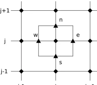
We compute velocity components and flux components at the staggered (cell-face-centered) points, shown in Fig. 4, from centered finite difference approximations of Eqs. (10) and (11). We use “compass” indices for such staggered val-ues, so that, for example, the “east” and “north” staggered water layer thicknesses are computed by averaging regular grid values:

We=

(W_i,jl +W_il_+1,j)

2 , Wn=

(W_i,jl +W_i,jl ₊₁)

2 . (39)

The nonlinear effective conductivityKfrom Eq. (9) is also needed at staggered locations. As a notational convenience defineR=P+ρwgband define these staggered-grid values (compare Mahaffy, 1976):

5e=

Ri+1,j−Ri,j 1x 2 +

Ri+1,j+1+Ri,j+1−Ri+1,j−1−Ri,j−1 41y 2 ,

5n=

Ri+1,j+1+Ri+1,j−Ri−1,j+1−Ri−1,j

41x 2 +

Ri,j+1−Ri,j 1y 2 . Thereby define

Ke=kWeα−15 (β−2)

2

e , Kn=kWnα−15 (β−2)

2

n . (40)

The velocity components(u, v)of the water velocityV are then found by differencing:

ue= −Ke

Ri+1,j−Ri,j

1x , vn= −Kn

Ri,j+1−Ri,j

i-1 i i+1 j-1 j j+1 w e s n

Figure 4. Numerical schemes Eqs. (44) and (49) use a grid-point-centered cell. Velocities, diffusivities, and fluxes are evaluated at staggered-grid locations (triangles at centers of cell edges) denoted by compass notatione, w, n, s. State functionsW, Wt il, P are lo-cated at regular grid points (diamonds).

For diffusivity we simply have

De=ρwgKeWe, Dn=ρwgKnWn. (42) We get the remaining staggered-grid quantities by shifting indices.

DefineQe(ue),Qw(uw),Qn(vn), andQs(vs)as the

face-centered (staggered-grid) normal components of the advec-tive flux VW; more detail is given in the next subsection. The grid values ofD= ∇ ·q= ∇ ·(VW )− ∇ ·(D∇W )using Eqs. (41) and (42) now become

Di,j =

Qe(ue)−Qw(uw)

1x +

Qn(vn)−Qs(vs)

1y (43)

−De(W

l

i+1,j−W l

i,j)−Dw(W l i,j−W

l i−1,j) 1x2

−

Dn(Wi,jl +1−Wi,jl )−Ds(Wi,jl −Wi,jl −1)

1y2 .

Local conservation is ensured by usingQe(ue)in computing

Di,j equal toQw(uw)used inDi+1,j, and so on.

Our scheme for approximating mass conservation Eq. (12) is

W_i,jl+1−W_i,jl

1t +

(Wtil)l_i,j+1−(Wtil)l_i,j

1t = −Di,j+

mij ρw

. (44) The updated value ofWtil, which appears on the left side of Eq. (44), is computed by trivial integration of Eq. (16), (Wtil)l_i,j+1=(Wtil)l_i,j+1t

_m

ij

ρw −Cd

. (45)

The given value W_till+1 is used if it is in the closed interval [0, W_tilmax], but otherwise the bounds 0≤Wtil≤W_tilmaxare en-forced. Once W_till+1 is computed, the value ofWl+1can be updated by Eq. (44) in a mass-conserving way.

Assuming no error in the flux components Q, the lo-cal truncation error (Morton and Mayers, 2005) of scheme Eq. (44) would beO(1t1+1x2+1y2)as an approxima-tion of Eq. (12). The actual truncaapproxima-tion error depends on the approximation of the discrete fluxes, addressed next. 6.2 Discrete advective fluxes

We test two flux-discretization schemes, namely, a first-order upwind scheme and the Koren flux-limited third-first-order scheme (Hundsdorfer and Verwer, 2003). Both schemes achieve non-oscillation and positivity, but with different lo-cal truncation error and complexity of implementation. The third-order scheme is best explained as a modification of our conservative (“donor cell”; LeVeque, 2002) first-order up-wind scheme.

For a flux-limited scheme, the following formulas apply in the casesue≥0,ue<0,vn≥0, andvn<0:

Qe(ue)=ueWi,j+9(θi)(Wi+1,j−Wi,j), (46) Qe(ue)=ue

h

Wi+1,j+9

(θi+1)−1

(Wi,j−Wi+1,j) i

,

Qn(vn)=vn

Wi,j+9(θj)(Wi,j+1−Wi,j)

,

Qn(vn)=vn

h

Wi,j+1+9

(θj+1)−1

(Wi,j−Wi,j+1)

i

,

where the subscriptedθquotients are

θi=

Wi,j−Wi−1,j

Wi+1,j−Wi,j

, θj=

Wi,j−Wi,j−1

Wi,j+1−Wi,j .

The first-order upwind scheme simply sets 9(θ )=0 in formulas Eq. (46). The Koren scheme limits its third-order and positive-coefficient correction to the upwind scheme by using this formula (Hundsdorfer and Verwer, 2003)

9(θ )=max

0,minn1, θ,1 3+

1 6θ

o

. (47)

When using the Koren flux limiter, the stencil in Fig. 4 is extended because regular grid neighbors Wi+2,j, Wi−2,j, Wi,j+2, Wi,j−2 are also involved in updating Wi,j. The

flux-correction-limited Koren third-order scheme bypasses the first-order limitation of positive linear finite difference– volume schemes imposed by Godunov’s barrier theorem (Hundsdorfer and Verwer, 2003, Sect. I.7.1) by using a non-linear correction formula. Though the Koren scheme is third-order where smoothness allows, it reverts to first-third-order at ex-trema and jumps whereθ1 orθ1.

For either scheme, if the water inputm is negative then we must actively enforce, by truncation, the positivity of the water thicknessW. In fact, positivity of the source-free advection–diffusion scheme, a desirable property which we can show by standard methods (Hundsdorfer and Verwer, 2003), does not ensure positivity of the solution if there is water removal, i.e., if _ρm

w− ∂Wtil

6.3 Discretization of the pressure equation

Pressure evolution Eq. (31) is a nonlinear diffusion with “re-action” terms from the opening and closing of cavities. How-ever, our numerical scheme for this equation is similar to the scheme for the mass-conservation equation (Sect. 6.1) be-cause the spatial derivatives are actually the same in each equation, namely,∇ ·q. Thus, we reuse the computation of those derivatives, namely, scheme Eq. (43), which givesDi,j.

Let Oij, Cij be the gridded values of the zeroth-order

(i.e., without spatial derivatives) opening and closing rates; see Eqs. (14), (15). Define the sum of all zeroth-order terms:

Zij=Cij−Oij+ mij

ρw

−(Wtil)

l+1

ij −(Wtil)lij

1t . (48)

Using Eq. (43) for the flux divergence, the scheme for pres-sure Eq. (31) is

φ0 ρwg

P_i,jl+1−P_i,jl

1t = −Di,j+Zij. (49)

Because Eq. (48) uses the updated value(Wtil)l_ij+1, Eq. (45) must be applied before Eq. (49) can be used to update P. There are also special cases at the boundaries of the region whereW >0; see Sect. 6.5.

6.4 Stability of time stepping

A sufficient condition for stability of mass-conservation scheme Eq. (44) comes from combining sufficient condi-tions for stability of the advection and diffusion parts. For the advection part we first define1tCFL, after the well-known Courant–Friedrichs–Lewy restriction for advection schemes (Morton and Mayers, 2005), by

1tCFL

_max|u|

1x +

max|v| 1y

=1

2, (50)

where V =(u, v) is the velocity of the water in the dis-tributed system. For the diffusion part we define1tWby

1tWmaxD

₁

1x2+ 1 1y2

=1

4. (51)

The condition 1t≤min{1tCFL, 1tW} is sufficient for sta-bility and convergence of scheme Eq. (44) if V,D, andm were all externally provided functions, i.e., in the case where Eqs. (32) are decoupled. We can show this by maximum prin-ciple arguments for the first-order upwind advection choice (Morton and Mayers, 2005), but standard theory at least sug-gests the same conclusion for the higher-order flux-limited advection scheme (Hundsdorfer and Verwer, 2003).

These time-step restrictions can be understood by consid-ering an example. We ran the model on a1x=1y=250 m grid to approximate steady state for the subglacial hydrology

of Nordenskiöldbreen (Van Pelt, 2013). We used realistic in-puts forH,b, andm, but a spatially constant ice sliding rate of |vb| =50 m a−1; other parameter values were from Ta-ble 1. The result is that the maximum computed water speed |V|is about 0.2 m s−1so Eq. (50) gives1tCFL≈300 s. Com-puted diffusivityD=ρwgKW has a maximum value that varies significantly in time, 0.1≤maxD≤5 m2s−1. Using a typical value maxD=1 m2s−1 in Eq. (51) gives1tW≈ 8000 s. Thus, in this simulation1tW≈251tCFL. This exam-ple suggests that, unless both the maximum speed|V|is un-usually low, and deep subglacial lakes develop so that maxD is large, the diffusive timescale is significantly longer than the CFL timescale. While the scaling 1tW=O(1x2) vs. 1tCFL=O(1x1)makes it clear that under sufficient spatial grid refinement1tWis controlling, we suspect that1tCFLis controlling for1x >100 m.

However, the time-step restriction from the pressure-equation scheme is typically shorter than either 1tW or 1tCFL. The time-step restriction for scheme Eq. (49) is com-parable to1tW, and we define1tPby

1tP

_2maxD

φ0

1 1x2+

1 1y2

=1. (52)

If the time step is set by

1t=min{1tCFL, 1tW, 1tP}, (53)

then we observe in practice that the coupled scheme consist-ing of Eqs. (44), (45), and (49) is stable.

Recalling Eq. (51), however, 1tP is actually a fraction of1tW, namely,1tP=2φ01tW. If we return to the above example for Nordenskiöldbreen, with φ0=0.01 we have 1tW≈8000 s,1tCFL≈300 s, and1tP≈160 s. In this case the pressure scheme has the shortest time step, but it is comparable to CFL. Because1tP is O(1x2), the pressure scheme restriction is certainly controlling for sufficiently fine grids. However, the time step1tP also scales with porosity φ0, so we can make it more or less severe by adjusting that parameter.

If implicit time stepping were instead used for the pressure equation, which would require overt variational inequality treatment to preserve physical pressure bounds (Schoof et al., 2012), then the timescales1tW, 1tCFLaddressed here would be the only restrictions. The time-step restriction1tWcould also be removed by implicit steps for the mass-conservation equation, though again this requires a variational inequality formulation because of the lower boundW≥0. Our obser-vation above that1tCFL1tWfor practical ice sheet grids suggests that implicit time stepping only for the diffusion part of the mass-conservation equation is not beneficial.

6.5 One time step of the model

For convenience only we denote the ice geometry, bed ge-ometry, and sliding speed (i.e.,Hi,j,bi,j,(Po)i,j, and|vb|i,j)

as though they are all time independent. The geometry may be quite general, with free land, floating ice shelf, or ice-free ocean allowed at any location(xi, yj). The geometry

in-put data determine boolean “masks” on the grid, based on 0 as the sea level elevation:

icefreei,j =(Hi,j=0)&(bi,j>0),

float_i,j =(ρiHi,j <−ρswbi,j),

whereρsw=1028.0 is sea-water density. Notefloati,j is

true both where there is floating ice shelf and where the ocean is ice free. The subglacial hydrology model exists only for grounded ice, that is, only if both flags icefreeand floatare false.

One time step follows this algorithm:

i. Start with values W_i,jl , (Wtil)li,j, Pi,jl which satisfy

boundsW≥0, 0≤Wtil≤W_tilmax, and 0≤P ≤Po. ii. Get(Wtil)l_i,j+1with Eq. (45). Enforce 0≤Wtil≤W_tilmax.

Ificefreei,j orfloati,j then set(Wtil)l_i,j+1=0. iii. Get W values averaged onto the staggered grid from

Eq. (39), staggered-grid values of the effective conduc-tivity K from Eq. (40), velocity components u, v at grid locations from Eq. (41), and staggered-grid values of the diffusivityDfrom Eq. (42).

iv. Get time step1tfrom Eq. (53).

v. Using Eq. (46) and a flux limiterψ (θ ), compute the ad-vective fluxesQe(αe)andQn(βn)at all staggered-grid points.

vi. Get flux divergence approximationsDi,j from Eq. (43).

vii. If icefreei,j then set P_i,jl+1=0. If floati,j then

setP_i,jl+1=(Po)i,j. IfWi,jl =0, and ificefreei,jand

floati,j are both false, then either setP_i,jl+1=(Po)i,j

(no sliding) or P_i,jl+1=0 (any sliding). Otherwise use Eq. (49) to computeP_i,jl+1.

viii. IfP_i,jl+1does not satisfy bounds 0≤P ≤Pothen trun-cate/project into this range.

ix. Ificefreei,j orfloati,j then setW_i,jl+1=0.

Other-wise use Eq. (44) to compute values forW_i,jl+1. x. IfW_i,jl+1<0 then truncate/project to getW_i,jl+1=0. xi. Update timetl+1=tl+1t and repeat at (i).

This algorithm goes with a reporting scheme for mass con-servation. Note that in steps (ii) and (ix) water is lost or gained at the margin where either the ice thickness goes to 0 on land (margins), or at locations where the ice becomes floating ice (grounding lines). Because such loss/gain may be the modeling goal – users want hydrological discharge – these amounts are reported. This reporting scheme also tracks the projections in step (x), which represent a mass-conservation error which goes to 0 in the continuum limit 1t→0.

6.6 Run-time options for hydrology models

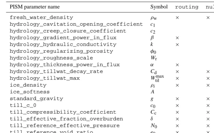
Option -hydrology NAME, where NAME is one of the three headings below, chooses the model equations.

distributed: this model is governed by the full set of Eqs. (32) in Sect. 5. The full set of parameters (Table 1) and variables (Table 2) are active in this model.

routing: in this reduced model the equation for pressure evolution is replaced byP =Po. The evolution equations for the state variablesW andWt il, and the bounds 0≤W and

0≤Wtil≤Wtilmax, are unchanged.

null: this further-reduced model is non-conserving. It has only the state variableWtil which is subject to bounds 0≤ Wtil≤Wtilmaxand evolves by Eq. (16).

The correspondence between the notation in this pa-per and PISM’s configurable parameters is shown in Ta-ble 3. These parameters can be set at runtime by us-ing the parameter name as an option, or by settus-ing a pism_overrides variable in a NetCDF file which is read with the-config_overrideoption (PISM authors, 2015). Filesrc/pism_config.cdl determines the de-fault values and units.

7 Results

7.1 Verification of the coupled model

By using the coupled, steady-state, nearly exact solution (Sect. 5.4) we verified most of the numerical schemes de-scribed above. (Verification is the process of measuring and analyzing the errors made by the numerical scheme, espe-cially as the numerical grid is refined (Wesseling, 2001).) To do this we initialized our time-stepping numerical scheme with the nearly exact steady solution and we measured the error relative to the exact values after 1 model month. The continuum time-dependent model Eq. (32) would cause no drift away from steady state, so any drift is numerical error. We did runs on grids decreasing by factors of 2 from 2 km to 125 m. Figure 5 shows the results based on the first-order upwind method for the fluxes.

Table 3. Correspondence between PISM parameter names and symbols in this paper (Table 1). All are used in thedistributedmodel, with indicated subsets used in theroutingandnullmodels.

PISM parameter name Symbol routing null

fresh_water_density ρw × ×

hydrology_cavitation_opening_coefficient c1

hydrology_creep_closure_coefficient c2

hydrology_gradient_power_in_flux β ×

hydrology_hydraulic_conductivity k ×

hydrology_regularizing_porosity φ0

hydrology_roughness_scale Wr

hydrology_thickness_power_in_flux α ×

hydrology_tillwat_decay_rate Cd × ×

hydrology_tillwat_max W_tilmax × ×

ice_density ρi × ×

ice_softness A

standard_gravity g × ×

till_c_0 c0 × ×

till_compressibility_coefficient Cc × ×

till_effective_fraction_overburden δ × ×

till_reference_effective_pressure N0 × ×

till_reference_void_ratio e0 × ×

0.001 0.01

error in W (m)

average W error maximum W error

125 250 500 1000 2000

0.01 0.1

∆ x (m)

error in P (bar)

average P error maximum P error

Figure 5. Average water thickness error |W−Wexact| decays as O(1x0.91), and average pressure error |P−Pexact| decays as

O(1x0.92), for grids with spacing 250≤1x=1y≤2000 m.

roughly linear (i.e., about O(1x1)) because the largest er-rors arise at locations of low regularity of the exact solution, including the radius r=5 km whereP quickly drops from Po, and at the ice sheet margin where there is a jump inWto 0.

The rates of convergence for average errors are nearly identical for the higher-resolution flux-limited scheme and for the first-order upwinding scheme (not shown). Because our problem is an advection–diffusion problem in which both the advection velocity and the diffusivity are

solution-dependent, it is difficult to separate the errors arising from numerical treatments of advection and diffusion. The first-order upwinding scheme for the advection has much larger numerical diffusivity but this diffusivity is masked by the physical diffusivity. Based on our verification evidence it is reasonable to choose the simpler first-order upwind method for applications, as it requires less interprocess communica-tion.

7.2 Application to the Greenland ice sheet

We now apply our hydrology models to the entire Greenland ice sheet at 2 km grid resolution. This nontrivial example demonstrates the model at large computational scale using real ice sheet geometry, with one-way coupling from ice dy-namics giving realistic distributions of overburden pressure, ice sliding speed, and basal melt rate.

7.2.1 Spun-up initial state

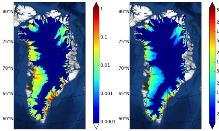
Figure 6. The inputs to the hydrology model are the modeled basal melt ratem/ρw(left; m a−1) and sliding speed|v_b|(right; m a−1) from the spun-up state.

Sheet Evolution (SeaRISE) data set for Greenland (Bind-schadler et al., 2013).

The spin-up grid sequence was to run 50 ka on a 20 km grid, 20 ka on a 10 km grid, 2 ka on a 5 km grid, and finally 200 a on a 2 km grid, with bilinear interpolation at each re-finement stage. The final 2 km stage, on a horizontal grid of 1.05 million grid points, used uniform 10 m vertical spacing so that the ice sheet flow was modeled on a structured 3-D grid of 460 million velocity–temperature points. This whole spin-up used 2800 total processor hours on 72 2.2 GHz AMD Opteron processors, a small computation for modern super-computers.

The results of this spin-up were validated by comparing results to present-day observations. In the last 100 a of this run the ice sheet volume varied by less than 0.04 %, so the model is in nearly steady state, though the actual Greenland ice sheet may not be as close to steady. The spun-up ice sheet volume of 3.094×106km3is close to the present-day volume of 3.088×106km3computed from the SeaRISE data on the same grid. Compared to volume alone, a better evaluation of dynamical quality is to compare the modeled and observed (Joughin et al., 2010) surface speed, with a very similar result to the comparison described in Aschwanden et al. (2013).

The spun-up initial state includes, in particular, modeled ice thicknessH, basal melt ratem, and sliding velocity|vb|; the latter two fields are shown in Figure 6. Areas of slid-ing roughly coincide with areas of basal melt because heat-producing (modeled) basal drag comes from the yield stress parameterized in Sect. 3.

7.2.2 Experimental setup and model runs

We used fields H, m, |vb| from the spun-up state as steady data in 5 model-year runs of the routing and distributedhydrology models; see Sect. 6.6 for model descriptions. Thus, only one-way coupling was tested: a steady ice dynamics model fed its fields to an evolving sub-glacial hydrology model. The hydrology model was initial-ized with the Wtil values from the spun-up state, but with W=0 initial values for both models, and alsoP =0 initial values fordistributed.

In the runs, variablesW,Wtil, andP were recomputed at each time step, at each of 1.05 million subglacial hydrology grid points, using parameter values from Table 1. In both routinganddistributedmodels the hydrological sys-tem became steady after the first 3 model years.

Figure 7. Outputs from theroutinghydrology model are the modeled till-stored water layer thicknessWtil(left; m) and modeled

trans-portable water layer thicknessW(right; m).

7.2.3 routingresults

The finalWtilandWfields from theroutingrun are shown in Fig. 7. The till is fully saturated (Wtil=2 m) in essen-tially all areas where basal melt occurs. In the outlet glacier areas the transportable water W concentrates along curves of steepest descent of the hydraulic potential; see detail in Fig. 8. The location of the pathways is determined primar-ily by the bedrock elevation detail provided by the SeaRISE data set, which is limited. Furthermore, the grid resolution of 2 km, while very high for whole ice sheet models, still causes spatial “smearing” of the flow pathways.

The continuum limit of the model would have concen-trated pathways of a few meters to tens of meters width. These concentrated pathways could be regarded as minimal “conduit-like” features of the subglacial hydrology. As noted in the introduction, however, our model has no “R-channel” conduit mechanism, in which dissipation heating of the flow-ing water generates wall melt back.

7.2.4 distributedresults

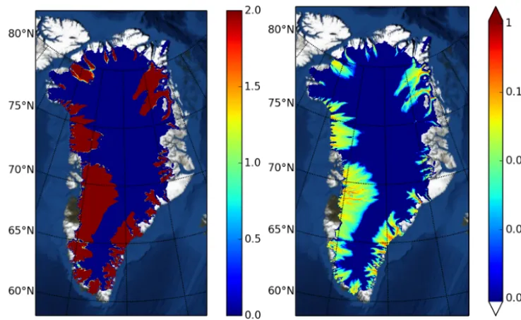
The final values ofW and the relative water pressureP /Po for the 5 model-year distributed run are shown in Fig. 9. The till is full (Wtil=2 m) in essentially all areas where basal melt occurs, so, asWtilis nearly identical to the routingresult, it is not shown.

Recall that |vb| determines the pressure drop caused by sliding-generated cavities. The effect is to spread out the wa-ter W relative to the routing model, as clearly seen in Fig. 9. There is now no strong concentration of W along curves of steepest descent of the hydraulic potential, but the

Figure 8. Detail of transportable waterWplotted in Fig. 7, cover-ing Jakobshavn (J), Helheim (H), and Kangerdlugssuaq (K) outlet glaciers.

spreading depends on opening and closing parameters in the distributedmodel, especially parametersc1, c2, φ0, Wr. Darcy flux model parametersα, β, kare also important. Pa-rameter identification using observed surface, in situ, basal reflectivity, discharge, and other data, though needed, is be-yond the scope of this paper.

Figure 9. Outputs from thedistributedhydrology model include the modeled transportable water layer thicknessW(left; m), and the modeled transportable water layer pressureP, shown relative to overburden pressure (i.e.,P /Po; right).

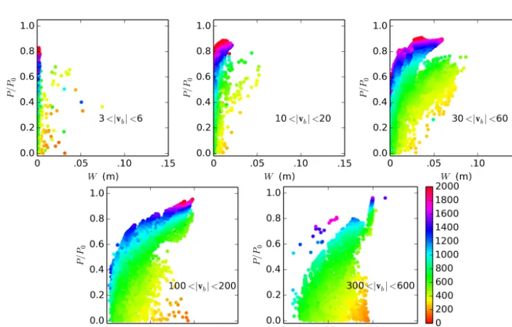
Figure 10. Scatter plots of(W, P /Po)pairs for all cells from thedistributedmodel run, which used roughness scaleWr=0.1 m. Each sub-plot only shows pairs from the indicated range of ice sliding speeds. Points are colored by ice thickness using a common scale shown beside last figure.

in each bin. While in the fast-sliding caseWis often compa-rable to the bed roughness scaleWr, for slow sliding we see generally lower water amounts (W.Wr/10) but a full range of pressures. In thick ice the pressureP is close to overbur-den even if there is fast sliding. Locations with high sliding,

8 Conclusions

This paper documents additions made to the Parallel Ice Sheet Model (PISM) in its 0.6 version released Febru-ary 2014. It describes and demonstrates a subglacial hydrol-ogy model which is novel in having these features:

– a 2-D parallel implementation of a coupled till-and-linked-cavities model;

– a pressure-equation regularization, using notional englacial porosity, which eases implementation and im-proves numerical performance;

– a scheme for maintaining physical pressure bounds (0≤ P ≤Po) at all times;

– verification using a nearly exact solution of the coupled mass-conservation and pressure equations, in the steady radial case;

– demonstration at high resolution and whole ice-sheet scale on a million-point hydrology grid.

Furthermore, the comprehensive exposition here clarifies the relationship among several pressure-determining “clo-sures” (Sect. 4), and it allows us to understand our model as a common extension of several seemingly disparate published models (Sect. 5). Additional analysis (Appendix A) shows that in steady state a functional relationship “P =P (W )” arises between pressure and water layer thickness. This anal-ysis reveals the diffusive nature of the apparently advective part of the steady-state flux.

Appendix A: Analysis of steady states

Relative to the time-dependent model Eqs. (32), steady-state Eqs. (35)–(38) have separate balances between the diver-gence of the flux and the water input, and the opening and closing processes. In particular, Eq. (38) allows us to write the pressureP =P (W )in steady state as a continuous func-tion of the layer thicknessW. However, steady state is only possible if a condition holds:

c1|vb|(Wr−W )+≤c2APo3W. (A1) This condition says that the maximum closing rateC(N, W ), which occurs at 0 water pressure, must equal or exceed the sliding-generated opening rateO(|vb|, W ).

We define a scaled basal sliding speed which has units of pressure; it is a scale for the pressure drop from cavitation:

sb=

_c

1|vb| c2A

1₃

. (A2)

Then Eq. (A1) is equivalent to the conditionW≥Wc, where Wc=

Wrsb3 (s_b3+P3

o)

is a critical water thickness. IfW≥Wcthen

P (W )=Po−sb

_(W

r−W )+ W

1₃

. (A3)

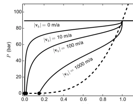
Formula Eq. (A3) applies even ifW≥Wr, in which caseP = Po. Under pressure (P =0) with subcritical water amount (W < Wc) does not occur in steady state, though it can occur in non-steady conditions; noteP (Wc)=0. Figure A1 shows the functionP (W )for different values of sliding speed|vb|, and Fig. A2 shows it for different values of overburden pres-surePo.

Flowers and Clarke (2002a) proposed functionPFC(W )– see Eq. (28) – for both steady and non-steady circumstances. Both functionsP (W )andPFC(W )are increasing, and both relateP to the overburden pressurePo. However, in Eq. (A3) the relation of P toPo is additive, while in Eq. (28) they are proportional. Power-law form Eq. (28) is not justified by the physical reasoning which led to Eq. (A3), even in steady state. It would appear that any functional relationshipP (W ) should also depend on the sliding velocity, as it does here, if cavitation influences the water pressure. In any case, in the current paper we do not impose a relationshipP =P (W )at all, though such a relation emerges in steady state.

We now consider how the steady-state water velocity V, and the associated fluxq, depends on other quantities. First, from Eqs. (35) and (A3), in steady state we have

∂P

∂W =

sbWr 3W43_(Wr−W )23

(A4)

ifWc< W < Wr. IfW≤Wcthen∂P /∂W is undefined, and ifW > Wrthen∂P /∂W =0. Formula Eq. (A4) and Figs. A1 and A2 agree that _∂W∂P → ∞asW%Wr.

0.0

0.2

0.4

0.6

0.8

1.0

W

(m)

0

20

40

60

80

100

P

(bar)

|

v

=

0 m/a

|

v

=

10 m/a

|

v

=

100 m/a

|

v

=

1000 m/a

Figure A1. The steady-state functionP (W )defined by Eq. (A3), usingWr=1 m andH=1000 m (solid curves). Values ofWcare indicated by black dots atP =0. For comparison, Flowers and Clarke (2002a) relation Eq. (28) is shown withWcrit=1 m (dashed

black).

0.0

0.2

0.4

0.6

0.8

1.0

W

(m)

0.0

0.2

0.4

0.6

0.8

1.0

P/P

o

H

=

2000 m

H

=

1000 m

H

=

500 m

H

=

200 m

Figure A2. The graph ofP (W )defined by Eq. (A3) also depends on overburden pressurePo=ρigH, shown using|vb| =100 m/a and Wr=1 m.

Now note that Eqs. (35), (A3), and (A4) imply a formula for the velocity in steady state:

V= −k

∇ψo−

_W

r−W W

1₃

∇sb (A5)

+ sbWr 3W43_(Wr−W )2/3

∇W

,

whereψo=Po+ρwgb. Thus, the direction of water veloc-ityV is determined by a combination of a geometric direc-tion (∇ψo), a direction derived from spatial variations in the