www.earth-syst-sci-data.net/7/289/2015/ doi:10.5194/essd-7-289-2015
© Author(s) 2015. CC Attribution 3.0 License.
Processing of water level derived from water pressure
data at the Time Series Station Spiekeroog
L. Holinde1, T. H. Badewien1, J. A. Freund1, E. V. Stanev1,2, and O. Zielinski1 1Institute for Chemistry and Biology of the Marine Environment, University of Oldenburg,
Carl-von-Ossietzky-Str. 9–11, 26129 Oldenburg, Germany
2Helmholtz-Zentrum Geesthacht, Max-Planck-Straße 1, 21502 Geesthacht, Germany
Correspondence to: L. Holinde (lars.holinde@uni-oldenbrg.de)
Received: 6 March 2015 – Published in Earth Syst. Sci. Data Discuss.: 13 April 2015 Revised: 25 August 2015 – Accepted: 2 October 2015 – Published: 27 October 2015
Abstract. The quality of water level time series data strongly varies with periods of high- and low-quality sensor data. In this paper we are presenting the processing steps which were used to generate high-quality water level data from water pressure measured at the Time Series Station (TSS) Spiekeroog. The TSS is positioned in a tidal inlet between the islands of Spiekeroog and Langeoog in the East Frisian Wadden Sea (southern North Sea). The processing steps will cover sensor drift, outlier identification, interpolation of data gaps and quality control. A central step is the removal of outliers. For this process an absolute threshold of 0.25 m 10 min−1 was selected which still keeps the water level increase and decrease during extreme events as shown during the quality control process. A second important feature of data processing is the interpolation of gappy data which is accomplished with a high certainty of generating trustworthy data. Applying these methods a 10-year data set (December 2002–December 2012) of water level information at the TSS was processed resulting in a 7-year time series (2005–2011). Supplementary data are available at doi:10.1594/PANGAEA.843740.
1 Introduction
The Time Series Station (TSS) Spiekeroog measures differ-ent time series data in the East Frisian Wadden Sea. The sta-tion is posista-tioned in the tidal inlet between the East Frisian islands Spiekeroog and Langeoog (Fig. 1, left) and has been measuring hydrographic, atmospheric and biological param-eters since 2002 (Reuter et al., 2009) as part of a long-term study of biogeochemical processes of tidal flats (Rullkötter, 2009). The goal of the Time Series Station was to have a plat-form at a fixed position for measurements during the whole year. Especially autumn and winter months were of interest because of extreme events.
Time series are often analysed for hindcast of events and trends in the past (Visser et al., 1996; Gräwe and Burchard, 2012). Due to the long-term aspect of these measurements data sets are often affected by sensor degradation and main-tenance resulting in time series combining periods of high-and low-quality of data. To assess the quality of the time
series data and to correct low-quality data sections differ-ent processing steps are needed. In this work we describe the processing of water pressure data recorded at the TSS Spiekeroog. The method emphasises the drift of sensor data and the handling of outliers and data gaps. At the end the quality of the data will be verified by frequency and storm surge analyses.
2 Instrumentation
Figure 1.Left: Time Series Station Spiekeroog in the tidal inlet between the East Frisian islands Spiekeroog and Langeoog. Right: schematic of the Time Series Station Spiekeroog with attached sensors; T: temperature sensor; C: conductivity sensor; P: pressure sensor, ADCP: acoustic Doppler current profiler, MST: Multispectral Transmissometer. (Badewien et al., 2009)
Table 1.Pressure sensors used between 2002 and 2012 at the Time Series Station Spiekeroog (FS: full scale).
Type Range Accuracy Drift
PDCR 901 0–30 dBar ±0.1 % FS ±0.1 % FS/a PDCR 4000 0–30 dBar ±0.08 % FS ±0.1 % FS/a PV-25L 0–30 dBar ±0.05 % FS ±0.1 % FS/a
later (26 September 2011) replaced with a PV-25L (Druck-und Durchflussmessung Peter Arbes e.K., Germany) due to a malfunction.
Data were processed and stored on the TSS. The pre-processing includes the conversion from measured currents to pressure data and binning of the measurement data to 1 min. In regular intervals the data were copied to a land-based computer. From this system the data were exported at an interval of 10 min for the time interval from 2003 to 2012 as monthly files.
3 Data Provenance and Structure
The data used in this paper are available at PANGAEA (doi:10.1594/PANGAEA.843740). The data were divided into yearly sections. Each section provides the original wa-ter pressure data (L1), the wawa-ter level afwa-ter the subtraction of a trend and removal of outliers (L2) and the final product of this paper the water level data, where gaps were interpo-lated (L3). In addition, each value is flagged with a bit coded
Table 2.Flag codes
Description Bit code
Trend subtracted 001
Outlier 010
Interpolated 100
value (Table 2) depending on the operations conducted with the value.
4 Methods
The data processing method is divided into four steps. For these steps meta-information about the time series, measure-ment station and nearby measuremeasure-ments is required. These steps are the following:
1. Subtraction of a trend
2. Removal of outliers
3. Calculation of supporting points and interpolation of missing data
4. Quality control of processed data
4.1 Subtraction of a trend
Figure 2.Measured water pressure data (blue) at the Time Series Station Spiekeroog before the validation and times of sensor main-tenance (red vertical lines).
(blue) and sensor maintenance (red) for the TSS Spiekeroog which dates are given in Appendix A in Tables A1 and A2. Each section is analysed for a trend by first calculating a run-ning mean for all data points and then deriving the trend of the result. These trends can result from short-term and long-term changes. Short-long-term changes are based on diurnal and semi-diurnals tidal cycles and wind stress. The long-term changes can be a result of sensor drift, bio-fouling, longer tidal cycles or sea level changes due to climate change.
If a strong decreasing trend is detected (Fig. 2, End 2011) this trend will be subtracted from the time series due to the high probability that this trend is based on sensor drift or bio-fouling. From other sections only the mean water level will be subtracted. The information which was subtracted from a section is given in Tables A1 and A2 in Appendix A.
During this step the transition from pressure data to wa-ter level data will also be performed for which the Gibbs Sea Water (GSW) Oceanographic Toolbox (V3.01, 11 May 2011) for MATLAB (R2014b, The MathWorks) was used. The toolbox is based on the International Thermodynamic Equa-tion of SeaWater – 2010 (TEOS-10, IOC, SCOR and IAPSO, 2010).
4.2 Removal of outliers
The next step of the data processing is to remove outliers. Outliers occur for example during sensor maintenance. To detect probable outliers the speed of water level change (gra-dient) between two adjacent data points is calculated. For this, the distribution of the gradients is presented in the his-togram of Fig. 3. Most values (99.96 %) have a maximum ab-solute gradient of 0.25 m for a1t of 10 min. Consequently, the probability is high that an absolute gradient exceeding 0.25 m 10 min−1is an outlier and should be removed. In
ad-Figure 3.The histogram is showing the gradient between two adja-cent data points. Vertical lines indicate the 0.25 m 10 min−1 thresh-old for the removal of outliers.
dition, each year is scanned visually in search for outliers missed by the gradient method.
4.3 Calculation of supporting points and interpolation of missing data
The removed outliers and gaps of the original time series rep-resent missing information making it more difficult to inter-pret the data set especially since many methods for the anal-ysis of time series require evenly sampled data (Karl et al., 1982). To fill these gaps an interpolation can be used. How-ever, for gaps longer than a tidal cycle dominated by the M2 tide the interpolated values might be wrong especially when using linear interpolation. Spline interpolation can also lead to wrong data due to overestimation or underestimation of zenith points. To prevent wrong data in these cases, it is pos-sible to calculate zenith points for the interpolation repre-senting the water level at high or low tide. These supporting points will be calculated by comparison with water level data from nearby measurement stations. In this case, a compari-son was made with water level data from Neuharlingersiel (53◦4200600N, 7◦4201500E) measured with a pressure sensor that can fall dry during spring low tide. In case of the sensor falling dry the value is not selected. For consistency, the first two steps of the data processing are also performed on the data from Neuharlingersiel.
Figure 4.The subfigures show the validation process for the year 2008. Top: the time series before the validation (blue) and sensor maintenance (red vertical lines) are shown. Middle: the time series (blue) and outliers (red) after the first two steps of the validation. Bottom: the time series after the interpolation (blue) and the com-parison data of Neuharlingersiel (red) are shown.
possible to calculate auxiliary supporting points for the inter-polation.
Tides can be described as a combination of cosine using a spline interpolation (MATLAB R2014b, function interp1 with spline method) the missing data points can be interpo-lated with a high certainty of achieving trustworthy data. For gaps longer than a tidal cycle (12.5 h) the prior calculated supporting points are used to avoid greater over and under estimation.
4.4 Quality control of processed data
Finally, to ensure the quality of the processed data a Fourier harmonic analysis and a storm flood analysis were per-formed. The Fourier harmonic analysis intends to show that it is possible to find all the main tidal frequencies and the difference between the original and the processed data. The storm flood analysis searches for severe short-term rises in the water level data. The German Hydrographic Institute (BSH, “Bundesamt für Schifffahrt und Hydrographie”) has published values for different magnitudes of storm floods at the German North Sea Coast (BSH, 2015). These values clas-sify a weak storm flood with water levels between 1.5 and 2.5 m above mean high water, a severe storm flood with wa-ter levels between 2.5 and 3.5 m and a very severe storm flood with water levels more than 3.5 m above mean high water.
June 2007
16 17 18 19 20 21 22 23 24 25 26 27 28 29 30
Figure 5.All three curves show data for 2 weeks in June 2007. The blue line shows the data after the removal of a trend and outliers and the red curve the interpolated data at the TSS Spiekeroog. The green curve shows data from Neuharlingersiel.
5 Results
The different processing steps were applied to the whole time series presented in Fig. 2. During the processing of the first three steps it became obvious that greater amounts of data and/or comparison measurements were missing in the first 2 years (2003 and 2004) and at the end of 2012. Following these observations these 3 years were excluded for further data processing in this work.
Examples of the results of the first four processing steps for data from 2008 are shown in Fig. 4. For the quality control the fully processed data set (2005–2011) will be used.
5.1 Data processing
Figure 4 presents the time series at different stages of the data processing for a time period from 1 January to 31 De-cember 2008. The top graph shows the measured pressure data before the validation (blue) and pressure sensor main-tenance (red). At the second vertical red line of the graph a shift in the water level is apparent and after the third a gap in the time series.
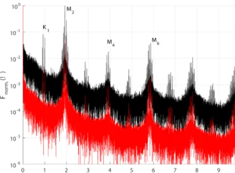
Figure 6. Fast Fourier Transformation (FFT) of the original (red) and processed (black) water level at Time Series Station Spiekeroog. K1: lunar diurnal constituent; M2: principal lunar semidiurnal constituent; M4 and M6: shallow water overtide of principal lunar semi-diurnal constituent.
The bottom graph of Fig. 4 shows the comparison with the water level data from Neuharlingersiel and the result of the interpolation of missing data. Figure 5 illustrates similar data for a shorter time period (15–31 June 2007). Both figures display only small differences in amplitude and time between the data from Neuharlingersiel and the Time Series Station. From the cross correlation the time difference was calculated with 20 min meaning that high/low water is earlier at the TSS than at Neuharlingersiel. A further comparison between the high/low tide of both measurement stations has shown that the delay mainly changes between 0 and 40 min with some outliers in both directions. In addition, this provided mean differences and standard deviation for high (0.00±0.17 m) and low (−0.03±0.20 m) water at both stations.
5.2 Data quality
Figure 6 shows the result of the Fourier transformation of the processed water level data (black) and the original data (red) for the years 2005 to 2011. The most influential tidal frequency is the M2tide and other semi-diurnal frequencies. The next most influential frequencies are the diurnal tides around the K1tide. Equally important for shallow coastal ar-eas are the M4and M6tides (Stanev et al., 2014). All of these peaks are much more pronounced in the processed time se-ries compared to the original. The highest peak in the original time series is directly at the beginning of the graph represent-ing the mean of data.
In Fig. 7 the storm flood analysis of the processed water level data is presented. To find and characterize the storm floods the mean high water was calculated with 1.33 m at the TSS. This leads to the discovery of six storm floods at the TSS Spiekeroog. These six storm floods can be characterized
Figure 7.Storm flood analysis of the water level data from the Time Series Station Spiekeroog (top) and Neuharlingersiel (bot-tom). Green marker: weak storm flood; red marker: severe storm flood; black marker: very severe storm flood.
as weak storm floods. The data from Neuharlingersiel (mean high water: 1.33 m) show eight storm events in the same time frame. Six of these storms can be characterized as a weak storm flood, one as a severe and one as very severe storm flood. Table 3 shows the water level during the storm floods above the mean high tide and the name of the storms.
6 Discussion
6.1 Subtraction of a trend
In the first processing step a piecewise linear trend or mean was subtracted. While it is easier to identify outliers by this way, it makes the data set more difficult to analyse for long-term sea level changes. The manual of the uti-lized pressure sensors states that the sensor degradation is ±0.1 % year−1 of a maximum of 30 dBar (Table 1). In winter 2008/2009 the water level date evinced a decrease by 0.8 dBar in 8 months. By contrast, the “Niedersäch-sische Landesbedtrieb für Wasserwirtschaft, Küsten- und Naturschutz” (NLWKN) has claimed that the water level is increasing (NLWKN, 2006). A possible reason for the de-creasing values of the water level is bio fouling which is es-pecially severe in spring and summer.
6.2 Removal of outliers
8 28/11/2011 Yoda 1.68 1.62
also lead to the removal of correct data if the water level is in-deed increasing very fast. A comparison between Fig. 4 and the results of the storm flood analysis (Fig. 7 and Table 3) shows that no values during extreme events were removed. In addition, Fig. 3 shows that about 99.96 % of all values have an absolute gradient lower than 0.25 m in 10 min for the TSS Spiekeroog. All of these pieces of information indicate that the selection of a gradient threshold of 0.025 m min−1is an acceptable choice for the measurement station in this study.
6.3 Calculation of supporting points and interpolation of missing data
A comparison between the time series data from Spiekeroog and Neuharlingersiel reveals that both are in good agree-ment. Constant values below −2 m at Neuharlingersiel are explained by the sensor falling dry during low water at spring tides. If one of these values would be taken as a support point then this could lead to an overestimation of the in-terpolated water level data. The cross correlation analysis reveals a 20 min time lag between the Time Series Station Spiekeroog and Neuharlingersiel since the tidal wave which moves through the North Sea reaches the station first. Com-paring high and low water at both stations this differences change mainly between 0 and 40 min with outlier in both di-rections. A comparison with the local tidal chart (BSH, 2011) shows a delay between Spiekeroog and Neuharlingersiel be-tween 1 and 5 min. The discrepancy could be a result of the 10 min sampling rate leading to possible errors of ±5 min. Another possibility is the influence of shallow water con-stituents on the tidal signal and the influence of wind. A scal-ing factor for the used water level data from Neuharlscal-ingersiel was not needed because only small differences were detected at high/low tide.
Sturges (1983) suggests that it is still possible to interpo-late data with gaps as long as 1/3 of the times series and a total number of missing values as high as half the time series. In this time series only 3.37 % of the data is missing. Using
data. These differences result from the previous processing steps and illustrate their usefulness.
Discrepancies in the storm flood events between the TSS Spiekeroog and Neuharlingersiel originate from the different positions of the measurement sites. During storm floods the wind blew from northern or western directions forcing the water into the harbour of Neuharlingersiel where it can ac-cumulate and lead to increased water levels. The water level is also increasing at the measurement station but here it is not possible for the water to pile up resulting in lower water levels than at Neuharlingersiel.
7 Conclusions
Processing water level data resulted in a relevant long-term data set. Here it should be emphasised that:
– From 99.96 % of the time series data only a linear trend was subtracted which leads to no difference in the ratio between the values.
– During the removal of outliers no values during extreme events were deleted. This was concluded derived from a comparison of storm floods between the Time Series Station Spiekeroog and Neuharlingersiel.
– The calculation of supporting points has yielded a mean 20 min time lag between the TSS Spiekeroog and Neuharlingersiel. This is greater than comparable data from the BSH and needs further analysis.
– The interpolated data follow the same trend as the mea-sured data at the TSS Spiekeroog.
All of the above shows that the described processing steps achieve good results if one accepts certain prerequisites. The first is that it will not be possible to analyse the wa-ter level time series with respect to changing sea levels be-cause of climate changes due to the removal of a trend. Still, it would be possible to compare the L2 and L1 data (doi:10.1594/PANGAEA.843740) to identify outliers in the L1 data set.
with a “*” behind the date.
Table A1. Maintenance times of the water level pressure sensor between December 2002 and January 2009. Dates marked with a “*” were not used during the trend removal.
Date Maintenance Sensor IDs
dd/mm/yyyy Primary Backup
17/12/2002 Sensor installation 40202 – 20/04/2004∗ Cleaning 40202 – 21/06/2004 Cleaning 40202 – 06/07/2004∗ Cleaning 40202 – 12/08/2004 Cleaning 40202 – 19/10/2004 Cleaning 40202 – 09/11/2004∗ Installation of backup sensor 40202 40301 01/01/2005 Change to backup sensor 40202 40301 18/07/2005∗ Cleaning – 40301 01/01/2006 Change to primary sensor 40202 40301 06/01/2006∗ Removal of backup sensor 40202 – 08/03/2006∗ Installation of backup sensor 40202 40301 01/04/2006 Cleaning 40202 40301 07/06/2006∗ Cleaning 40202 40301 29/09/2006∗ Cleaning 40202 40301 10/10/2006∗ Cleaning 40202 40301 26/03/2007 Sensor Exchange (primary) 40301 – 18/04/2007∗ Cleaning 40301 – 23/05/2007∗ Cleaning 40301 – 04/10/2007 Sensor Exchange (primary) 40202 – 09/10/2007∗ Cleaning 40202 – 19/10/2007 Sensor Exchange (primary) 40301 40202 04/12/2007∗ Cleaning 40202 40301 14/07/2008∗ Sensor Exchange (backup) 40301 40801 09/09/2008 Sensor Exchange (primary) 40202 40801 16/09/2008∗ Sensor Exchange (backup) 40202 40301 21/01/2009 Sensor Exchange (primary) 40801 40301
Acknowledgements. Special thanks to Axel Braun and Walde-mar Siewert for the maintenance on the station during the whole year and all weather conditions as well as for Helmo Nikolai for servicing the institute boats. The authors are grateful to Rainer Reuter for the concept and construction of the Time Series Station Spiekeroog.
Part of the data was acquired during the project BioGeoChem-istry of Tidal Flats (DFG, grant no. FOR 432).
Edited by: F. Schmitt
References
Badewien, T. H., Zimmer, E., Bartholoma, A., and Reuter, R.: To-wards continuous long-term measurements of suspended partic-ulate matter (SPM) in turbid coastal waters, Ocean Dynam., 59, 227–238, doi:10.1007/s10236-009-0183-8, 2009.
BSH: Gezeitenkalender 2011, Hoch- und Niedrigwasserzeiten für die Deutsche Bucht und deren Flussgebiete, Hamburg, Germany, 2011.
BSH: Informationen zu Sturmfluten, available at: http://www.bsh. de/de/Meeresdaten/Vorhersagen/Sturmfluten/, last access: 20 January 2015.
Gräwe, U. and Burchard, H.: Storm surges in the Western Baltic Sea: the present and a possible future, Clim. Dynam., 39, 165– 183, 2012.
IOC, SCOR and IAPSO: The international thermodynamic equa-tion of seawater – 2010: Calculaequa-tion and use of thermodynamic properties, Report, Unesco, Paris, France, 2010.
Karl, T. R., Koscielny, A. J., and Diaz, H. F.: Potential errors in the application of principal component (eigenvector) anal-ysis to geophysical data, J. Appl. Meteorol., 21, 1183–1186, doi:10.1175/1520-0450(1982)021<1183:PEITAO>2.0.CO;2, 1982.
NLWKN: Jahresbericht 2005 des NLWKN, Report, Nieder-sächsischer Landesbetrieb für Wasserwirtschaft, Küsten- und Naturschutz, Norden, Germany, 2006.
Reuter, R., Badewien, T. H., Bartholomä, A., Braun, A., Lübben, A., and Rullkötter, J.: A hydrographic time series station in the Wad-den Sea (southern North Sea), Ocean Dynam., 59, 195–211, doi:10.1007/s10236-009-0196-3, 2009.
Rullkötter, J.: The back-barrier tidal flats in the southern North Sea a multidisciplinary approach to reveal the main driv-ing forces shapdriv-ing the system, Ocean Dynam., 59, 157–165, doi:10.1007/s10236-009-0197-2, 2009.
Stanev, E. V., Al-Nadhairi, R., Staneva, J., Schulz-Stellenfleth, J., and Valle-Levinson, A.: Tidal wave transformations in the Ger-man Bight, Ocean Dynam., 64, 951–968, doi:10.1007/s10236-014-0733-6, 2014.
Sturges, W.: On interpolating gappy records for time-series analysis, J. Geophys. Res.-Oceans, 88, 9736–9740, doi:10.1029/Jc088ic14p09736, 1983.