A tutorial on Principal Components Analysis
Lindsay I Smith
Chapter 1
Introduction
This tutorial is designed to give the reader an understanding of Principal Components Analysis (PCA). PCA is a useful statistical technique that has found application in fields such as face recognition and image compression, and is a common technique for finding patterns in data of high dimension.
Before getting to a description of PCA, this tutorial first introduces mathematical concepts that will be used in PCA. It covers standard deviation, covariance, eigenvec-tors and eigenvalues. This background knowledge is meant to make the PCA section very straightforward, but can be skipped if the concepts are already familiar.
Chapter 2
Background Mathematics
This section will attempt to give some elementary background mathematical skills that will be required to understand the process of Principal Components Analysis. The topics are covered independently of each other, and examples given. It is less important to remember the exact mechanics of a mathematical technique than it is to understand the reason why such a technique may be used, and what the result of the operation tells us about our data. Not all of these techniques are used in PCA, but the ones that are not explicitly required do provide the grounding on which the most important techniques are based.
I have included a section on Statistics which looks at distribution measurements, or, how the data is spread out. The other section is on Matrix Algebra and looks at eigenvectors and eigenvalues, important properties of matrices that are fundamental to PCA.
2.1
Statistics
The entire subject of statistics is based around the idea that you have this big set of data, and you want to analyse that set in terms of the relationships between the individual points in that data set. I am going to look at a few of the measures you can do on a set of data, and what they tell you about the data itself.
2.1.1
Standard Deviation
of some bigger population. There is a reference later in this section pointing to more information about samples and populations.
Here’s an example set:
I could simply use the symbol to refer to this entire set of numbers. If I want to refer to an individual number in this data set, I will use subscripts on the symbol to indicate a specific number. Eg.
refers to the 3rd number in , namely the number 4. Note that
is the first number in the sequence, not
like you may see in some textbooks. Also, the symbol will be used to refer to the number of elements in the
set
There are a number of things that we can calculate about a data set. For example, we can calculate the mean of the sample. I assume that the reader understands what the mean of a sample is, and will only give the formula:
!"$#
"
Notice the symbol
(said “X bar”) to indicate the mean of the set . All this formula says is “Add up all the numbers and then divide by how many there are”.
Unfortunately, the mean doesn’t tell us a lot about the data except for a sort of middle point. For example, these two data sets have exactly the same mean (10), but are obviously quite different:
&%'&%( *)
+,
So what is different about these two sets? It is the spread of the data that is different. The Standard Deviation (SD) of a data set is a measure of how spread out the data is.
How do we calculate it? The English definition of the SD is: “The average distance from the mean of the data set to a point”. The way to calculate it is to compute the squares of the distance from each data point to the mean of the set, add them all up, divide by
, and take the positive square root. As a formula:
/
!"$# 10
"
3254
0
-2
Where/
is the usual symbol for standard deviation of a sample. I hear you asking “Why are you using0
6-2
and not ?”. Well, the answer is a bit complicated, but in general,
if your data set is a sample data set, ie. you have taken a subset of the real-world (like surveying 500 people about the election) then you must use0
7-2
because it turns out that this gives you an answer that is closer to the standard deviation that would result if you had used the entire population, than if you’d used . If, however, you are not
calculating the standard deviation for a sample, but for an entire population, then you should divide by instead of
0
8-2
. For further reading on this topic, the web page
http://mathcentral.uregina.ca/RR/database/RR.09.95/weston2.html describes standard
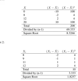
Set 1:
0
32
0
32
4
0 -10 100
8 -2 4
12 2 4
20 10 100
Total 208
Divided by (n-1) 69.333
Square Root 8.3266
Set 2:
"
0
"
32
0
"
32
4
8 -2 4
9 -1 1
11 1 1
12 2 4
Total 10
Divided by (n-1) 3.333
[image:5.612.142.402.81.353.2]Square Root 1.8257
Table 2.1: Calculation of standard deviation
difference between each of the denominators. It also discusses the difference between samples and populations.
So, for our two data sets above, the calculations of standard deviation are in Ta-ble 2.1.
And so, as expected, the first set has a much larger standard deviation due to the fact that the data is much more spread out from the mean. Just as another example, the data set:
%%&%&%
also has a mean of 10, but its standard deviation is 0, because all the numbers are the same. None of them deviate from the mean.
2.1.2
Variance
Variance is another measure of the spread of data in a data set. In fact it is almost identical to the standard deviation. The formula is this:
/
4
!"9# 0
"
32
4
0
You will notice that this is simply the standard deviation squared, in both the symbol (/
4
) and the formula (there is no square root in the formula for variance). /
4
is the usual symbol for variance of a sample. Both these measurements are measures of the spread of the data. Standard deviation is the most common measure, but variance is also used. The reason why I have introduced variance in addition to standard deviation is to provide a solid platform from which the next section, covariance, can launch from.
Exercises
Find the mean, standard deviation, and variance for each of these data sets.
;
[12 23 34 44 59 70 98]
;
[12 15 25 27 32 88 99]
;
[15 35 78 82 90 95 97]
2.1.3
Covariance
The last two measures we have looked at are purely 1-dimensional. Data sets like this could be: heights of all the people in the room, marks for the last COMP101 exam etc. However many data sets have more than one dimension, and the aim of the statistical analysis of these data sets is usually to see if there is any relationship between the dimensions. For example, we might have as our data set both the height of all the students in a class, and the mark they received for that paper. We could then perform statistical analysis to see if the height of a student has any effect on their mark.
Standard deviation and variance only operate on 1 dimension, so that you could only calculate the standard deviation for each dimension of the data set independently of the other dimensions. However, it is useful to have a similar measure to find out how much the dimensions vary from the mean with respect to each other.
Covariance is such a measure. Covariance is always measured between 2 dimen-sions. If you calculate the covariance between one dimension and itself, you get the variance. So, if you had a 3-dimensional data set (< ,= ,> ), then you could measure the
covariance between the< and= dimensions, the< and> dimensions, and the= and>
dimensions. Measuring the covariance between< and< , or= and= , or> and> would
give you the variance of the< ,= and> dimensions respectively.
The formula for covariance is very similar to the formula for variance. The formula for variance could also be written like this:
?
(+@
0
A2 !"9# 0
"
32
0
"
A2
0
:-2
where I have simply expanded the square term to show both parts. So given that knowl-edge, here is the formula for covariance:
B&CD?
0
8E+F2G !"9# 0
"
32
0
F
"
F2
0
includegraphicscovPlot.ps
Figure 2.1: A plot of the covariance data showing positive relationship between the number of hours studied against the mark received
It is exactly the same except that in the second set of brackets, the ’s are replaced by
F
’s. This says, in English, “For each data item, multiply the difference between the<
value and the mean of< , by the the difference between the= value and the mean of= .
Add all these up, and divide by0
.-2
”.
How does this work? Lets use some example data. Imagine we have gone into the world and collected some 2-dimensional data, say, we have asked a bunch of students how many hours in total that they spent studying COSC241, and the mark that they received. So we have two dimensions, the first is theH dimension, the hours studied,
and the second is theI dimension, the mark received. Figure 2.2 holds my imaginary
data, and the calculation of B&CD?
0
H
E
I
2
, the covariance between the Hours of study done and the Mark received.
So what does it tell us? The exact value is not as important as it’s sign (ie. positive or negative). If the value is positive, as it is here, then that indicates that both di-mensions increase together, meaning that, in general, as the number of hours of study increased, so did the final mark.
If the value is negative, then as one dimension increases, the other decreases. If we had ended up with a negative covariance here, then that would have said the opposite, that as the number of hours of study increased the the final mark decreased.
In the last case, if the covariance is zero, it indicates that the two dimensions are independent of each other.
The result that mark given increases as the number of hours studied increases can be easily seen by drawing a graph of the data, as in Figure 2.1.3. However, the luxury of being able to visualize data is only available at 2 and 3 dimensions. Since the co-variance value can be calculated between any 2 dimensions in a data set, this technique is often used to find relationships between dimensions in high-dimensional data sets where visualisation is difficult.
You might ask “isB1CD?
0
8E1F,2
equal toB&CD?
0
FJEKA2
”? Well, a quick look at the for-mula for covariance tells us that yes, they are exactly the same since the only dif-ference betweenB1CD?
0
8E1F,2
andB&CD?
0
FLEMN2
is that 0
" A2 0 F " F72
is replaced by
0 F " F2 0 " A2
. And since multiplication is commutative, which means that it doesn’t matter which way around I multiply two numbers, I always get the same num-ber, these two equations give the same answer.
2.1.4
The covariance Matrix
Recall that covariance is always measured between 2 dimensions. If we have a data set with more than 2 dimensions, there is more than one covariance measurement that can be calculated. For example, from a 3 dimensional data set (dimensions< ,= , > ) you
could calculateB&CD?
0 < E = 2 ,0 B&CD? 0 < E > 2
, andB&CD?
0
=
E
>
2
. In fact, for an -dimensional data
set, you can calculate !PO
Q
!SR 4DT
OU
Hours(H) Mark(M)
Data 9 39
15 56
25 93
14 61
10 50
18 75
0 32
16 85
5 42
19 70
16 66
20 80
Totals 167 749
Averages 13.92 62.42
Covariance:
H I
0
H
"
H
2
0
I
"
I
2
0
H
"
H
2
0
I
"
I
2
9 39 -4.92 -23.42 115.23
15 56 1.08 -6.42 -6.93
25 93 11.08 30.58 338.83
14 61 0.08 -1.42 -0.11
10 50 -3.92 -12.42 48.69
18 75 4.08 12.58 51.33
0 32 -13.92 -30.42 423.45
16 85 2.08 22.58 46.97
5 42 -8.92 -20.42 182.15
19 70 5.08 7.58 38.51
16 66 2.08 3.58 7.45
20 80 6.08 17.58 106.89
Total 1149.89
[image:8.612.229.382.126.312.2]Average 104.54
A useful way to get all the possible covariance values between all the different dimensions is to calculate them all and put them in a matrix. I assume in this tutorial that you are familiar with matrices, and how they can be defined. So, the definition for the covariance matrix for a set of data with dimensions is:
V !PWS! 0 B "MXY E B "ZXY B&CD? 0M[]\_^ " E [`\Z^ Y 2a2ME where V
!PWS! is a matrix with
rows and columns, and [`\Z^b
is the< th dimension.
All that this ugly looking formula says is that if you have an -dimensional data set,
then the matrix has rows and columns (so is square) and each entry in the matrix is
the result of calculating the covariance between two separate dimensions. Eg. the entry on row 2, column 3, is the covariance value calculated between the 2nd dimension and the 3rd dimension.
An example. We’ll make up the covariance matrix for an imaginary 3 dimensional data set, using the usual dimensions< ,= and> . Then, the covariance matrix has 3 rows
and 3 columns, and the values are this:
V B&CD? 0 < E < 2 B&CD? 0 < E = 2 B&CD? 0 < E > 2 B&CD? 0 = E < 2 B&CD? 0 = E = 2 B&CD? 0 = E > 2 B&CD? 0 > E < 2 B&CD? 0 > E = 2 B&CD? 0 > E > 2
Some points to note: Down the main diagonal, you see that the covariance value is between one of the dimensions and itself. These are the variances for that dimension. The other point is that sinceB&CD?
0
(E+c+2 B1CD?
0
c&E1(P2
, the matrix is symmetrical about the main diagonal.
Exercises
Work out the covariance between the< and= dimensions in the following 2
dimen-sional data set, and describe what the result indicates about the data.
Item Number: 1 2 3 4 5
< 10 39 19 23 28 = 43 13 32 21 20
Calculate the covariance matrix for this 3 dimensional set of data.
Item Number: 1 2 3
< 1 -1 4 = 2 1 3 > 1 3 -1
2.2
Matrix Algebra
f d
ed f
d
g
f
d
[image:10.612.212.403.83.156.2]
Figure 2.2: Example of one non-eigenvector and one eigenvector
f
d
ed
f
g
f
Figure 2.3: Example of how a scaled eigenvector is still and eigenvector
2.2.1
Eigenvectors
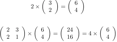
As you know, you can multiply two matrices together, provided they are compatible sizes. Eigenvectors are a special case of this. Consider the two multiplications between a matrix and a vector in Figure 2.2.
In the first example, the resulting vector is not an integer multiple of the original vector, whereas in the second example, the example is exactly 4 times the vector we began with. Why is this? Well, the vector is a vector in 2 dimensional space. The
vector
d
(from the second example multiplication) represents an arrow pointing
from the origin, 0 %SEh%2
, to the point 0 dSEh2
. The other matrix, the square one, can be thought of as a transformation matrix. If you multiply this matrix on the left of a vector, the answer is another vector that is transformed from it’s original position.
It is the nature of the transformation that the eigenvectors arise from. Imagine a transformation matrix that, when multiplied on the left, reflected vectors in the line
=
< . Then you can see that if there were a vector that lay on the line=
< , it’s
reflection it itself. This vector (and all multiples of it, because it wouldn’t matter how long the vector was), would be an eigenvector of that transformation matrix.
What properties do these eigenvectors have? You should first know that eigenvec-tors can only be found for square matrices. And, not every square matrix has eigen-vectors. And, given an
f
matrix that does have eigenvectors, there are of them.
Given ad
f
d
matrix, there are 3 eigenvectors.
[image:10.612.210.403.208.278.2]not changing it’s direction. Lastly, all the eigenvectors of a matrix are perpendicular, ie. at right angles to each other, no matter how many dimensions you have. By the way, another word for perpendicular, in maths talk, is orthogonal. This is important because it means that you can express the data in terms of these perpendicular eigenvectors, instead of expressing them in terms of the< and= axes. We will be doing this later in
the section on PCA.
Another important thing to know is that when mathematicians find eigenvectors, they like to find the eigenvectors whose length is exactly one. This is because, as you know, the length of a vector doesn’t affect whether it’s an eigenvector or not, whereas the direction does. So, in order to keep eigenvectors standard, whenever we find an eigenvector we usually scale it to make it have a length of 1, so that all eigenvectors have the same length. Here’s a demonstration from our example above.
d
is an eigenvector, and the length of that vector is
0
d
4i
4
2kj ld
so we divide the original vector by this much to make it have a length of 1.
d
m j dn
dSo j &d So j &d
How does one go about finding these mystical eigenvectors? Unfortunately, it’s only easy(ish) if you have a rather small matrix, like no bigger than about
d
f
d
. After that, the usual way to find the eigenvectors is by some complicated iterative method which is beyond the scope of this tutorial (and this author). If you ever need to find the eigenvectors of a matrix in a program, just find a maths library that does it all for you. A useful maths package, called newmat, is available at http://webnz.com/robert/ .
Further information about eigenvectors in general, how to find them, and orthogo-nality, can be found in the textbook “Elementary Linear Algebra 5e” by Howard Anton, Publisher John Wiley & Sons Inc, ISBN 0-471-85223-6.
2.2.2
Eigenvalues
Eigenvalues are closely related to eigenvectors, in fact, we saw an eigenvalue in Fig-ure 2.2. Notice how, in both those examples, the amount by which the original vector was scaled after multiplication by the square matrix was the same? In that example, the value was 4. 4 is the eigenvalue associated with that eigenvector. No matter what multiple of the eigenvector we took before we multiplied it by the square matrix, we would always get 4 times the scaled vector as our result (as in Figure 2.3).
Exercises
For the following square matrix:
d %
-p%
Decide which, if any, of the following vectors are eigenvectors of that matrix and give the corresponding eigenvalue.
%
d
%
%
d
Chapter 3
Principal Components Analysis
Finally we come to Principal Components Analysis (PCA). What is it? It is a way of identifying patterns in data, and expressing the data in such a way as to highlight their similarities and differences. Since patterns in data can be hard to find in data of high dimension, where the luxury of graphical representation is not available, PCA is a powerful tool for analysing data.
The other main advantage of PCA is that once you have found these patterns in the data, and you compress the data, ie. by reducing the number of dimensions, without much loss of information. This technique used in image compression, as we will see in a later section.
This chapter will take you through the steps you needed to perform a Principal Components Analysis on a set of data. I am not going to describe exactly why the technique works, but I will try to provide an explanation of what is happening at each point so that you can make informed decisions when you try to use this technique yourself.
3.1
Method
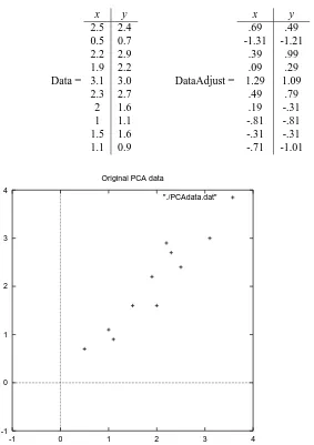
Step 1: Get some data
In my simple example, I am going to use my own made-up data set. It’s only got 2 dimensions, and the reason why I have chosen this is so that I can provide plots of the data to show what the PCA analysis is doing at each step.
The data I have used is found in Figure 3.1, along with a plot of that data.
Step 2: Subtract the mean
For PCA to work properly, you have to subtract the mean from each of the data dimen-sions. The mean subtracted is the average across each dimension. So, all the< values
have
< (the mean of the< values of all the data points) subtracted, and all the= values
have
Data =
x y
2.5 2.4 0.5 0.7 2.2 2.9 1.9 2.2 3.1 3.0 2.3 2.7 2 1.6 1 1.1 1.5 1.6 1.1 0.9
DataAdjust =
x y
.69 .49 -1.31 -1.21
.39 .99 .09 .29 1.29 1.09
.49 .79 .19 -.31 -.81 -.81 -.31 -.31 -.71 -1.01
-1 0 1 2 3 4
-1 0 1 2 3 4
Original PCA data
[image:14.612.143.426.126.527.2]"./PCAdata.dat"
Step 3: Calculate the covariance matrix
This is done in exactly the same way as was discussed in section 2.1.4. Since the data is 2 dimensional, the covariance matrix will be
f
. There are no surprises here, so I will just give you the result:
B&CD? q
r
q
r
q
r
q
So, since the non-diagonal elements in this covariance matrix are positive, we should expect that both the< and= variable increase together.
Step 4: Calculate the eigenvectors and eigenvalues of the covariance
matrix
Since the covariance matrix is square, we can calculate the eigenvectors and eigenval-ues for this matrix. These are rather important, as they tell us useful information about our data. I will show you why soon. In the meantime, here are the eigenvectors and eigenvalues:
s
\Zt
s
?
(uwv sx/
q
% %dd
q
%
s
\_t
s
?rsyBZz1C
@
/
-q
d
-q
&dd
q
r&dd
-q
d&
It is important to notice that these eigenvectors are both unit eigenvectors ie. their lengths are both 1. This is very important for PCA, but luckily, most maths packages, when asked for eigenvectors, will give you unit eigenvectors.
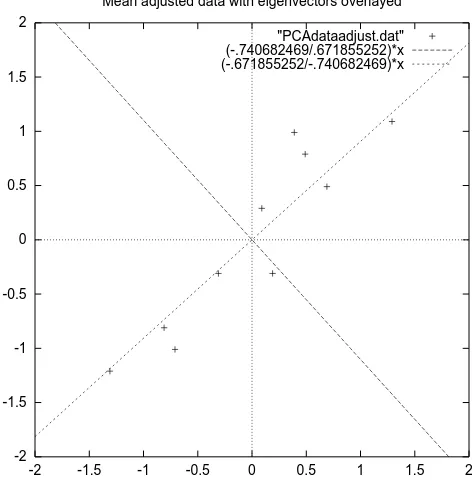
So what do they mean? If you look at the plot of the data in Figure 3.2 then you can see how the data has quite a strong pattern. As expected from the covariance matrix, they two variables do indeed increase together. On top of the data I have plotted both the eigenvectors as well. They appear as diagonal dotted lines on the plot. As stated in the eigenvector section, they are perpendicular to each other. But, more importantly, they provide us with information about the patterns in the data. See how one of the eigenvectors goes through the middle of the points, like drawing a line of best fit? That eigenvector is showing us how these two data sets are related along that line. The second eigenvector gives us the other, less important, pattern in the data, that all the points follow the main line, but are off to the side of the main line by some amount.
So, by this process of taking the eigenvectors of the covariance matrix, we have been able to extract lines that characterise the data. The rest of the steps involve trans-forming the data so that it is expressed in terms of them lines.
Step 5: Choosing components and forming a feature vector
-2 -1.5 -1 -0.5 0 0.5 1 1.5 2
-2 -1.5 -1 -0.5 0 0.5 1 1.5 2 Mean adjusted data with eigenvectors overlayed
[image:16.612.145.381.210.452.2]"PCAdataadjust.dat" (-.740682469/.671855252)*x (-.671855252/-.740682469)*x
will notice that the eigenvalues are quite different values. In fact, it turns out that the eigenvector with the highest eigenvalue is the principle component of the data set. In our example, the eigenvector with the larges eigenvalue was the one that pointed down the middle of the data. It is the most significant relationship between the data dimensions.
In general, once eigenvectors are found from the covariance matrix, the next step is to order them by eigenvalue, highest to lowest. This gives you the components in order of significance. Now, if you like, you can decide to ignore the components of lesser significance. You do lose some information, but if the eigenvalues are small, you don’t lose much. If you leave out some components, the final data set will have less dimensions than the original. To be precise, if you originally have dimensions in
your data, and so you calculate eigenvectors and eigenvalues, and then you choose
only the first{ eigenvectors, then the final data set has only{ dimensions.
What needs to be done now is you need to form a feature vector, which is just a fancy name for a matrix of vectors. This is constructed by taking the eigenvectors that you want to keep from the list of eigenvectors, and forming a matrix with these eigenvectors in the columns.
| s ( z v@ sy}~syBZz1C @n 0 s \Zt s \Zt 4 s \Zt qqqq s \Zt ! 2
Given our example set of data, and the fact that we have 2 eigenvectors, we have two choices. We can either form a feature vector with both of the eigenvectors:
-q r&dd -q &d -q &dr q &dd
or, we can choose to leave out the smaller, less significant component and only have a single column: -q &dd -q d&
We shall see the result of each of these in the next section.
Step 5: Deriving the new data set
This the final step in PCA, and is also the easiest. Once we have chosen the components (eigenvectors) that we wish to keep in our data and formed a feature vector, we simply take the transpose of the vector and multiply it on the left of the original data set, transposed. | \ (u [ ( z (6k CD | s ( z v@ sx}7syBZz1C @ f CD [ ( z ( ) v /hz E where CD | s ( z v@ sy}6syBZz1C @
is the matrix with the eigenvectors in the columns
trans-posed so that the eigenvectors are now in the rows, with the most significant
eigenvec-tor at the top, and CD [ ( z ( ) v /hz
easier if we take the transpose of the feature vector and the data first, rather that having a little T symbol above their names from now on.|
\
(u
[
(
z
(
is the final data set, with data items in columns, and dimensions along rows.
What will this give us? It will give us the original data solely in terms of the vectors
we chose. Our original data set had two axes,< and= , so our data was in terms of
them. It is possible to express data in terms of any two axes that you like. If these axes are perpendicular, then the expression is the most efficient. This was why it was important that eigenvectors are always perpendicular to each other. We have changed our data from being in terms of the axes< and= , and now they are in terms of our 2
eigenvectors. In the case of when the new data set has reduced dimensionality, ie. we have left some of the eigenvectors out, the new data is only in terms of the vectors that we decided to keep.
To show this on our data, I have done the final transformation with each of the possible feature vectors. I have taken the transpose of the result in each case to bring the data back to the nice table-like format. I have also plotted the final points to show how they relate to the components.
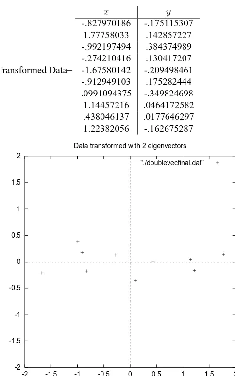
In the case of keeping both eigenvectors for the transformation, we get the data and the plot found in Figure 3.3. This plot is basically the original data, rotated so that the eigenvectors are the axes. This is understandable since we have lost no information in this decomposition.
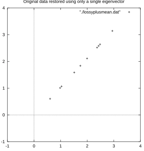
The other transformation we can make is by taking only the eigenvector with the largest eigenvalue. The table of data resulting from that is found in Figure 3.4. As expected, it only has a single dimension. If you compare this data set with the one resulting from using both eigenvectors, you will notice that this data set is exactly the first column of the other. So, if you were to plot this data, it would be 1 dimensional, and would be points on a line in exactly the< positions of the points in the plot in
Figure 3.3. We have effectively thrown away the whole other axis, which is the other eigenvector.
So what have we done here? Basically we have transformed our data so that is expressed in terms of the patterns between them, where the patterns are the lines that most closely describe the relationships between the data. This is helpful because we have now classified our data point as a combination of the contributions from each of those lines. Initially we had the simple< and= axes. This is fine, but the< and=
values of each data point don’t really tell us exactly how that point relates to the rest of the data. Now, the values of the data points tell us exactly where (ie. above/below) the trend lines the data point sits. In the case of the transformation using both eigenvectors, we have simply altered the data so that it is in terms of those eigenvectors instead of the usual axes. But the single-eigenvector decomposition has removed the contribution due to the smaller eigenvector and left us with data that is only in terms of the other.
3.1.1
Getting the old data back
Wanting to get the original data back is obviously of great concern if you are using the PCA transform for data compression (an example of which to will see in the next section). This content is taken from
Transformed Data=
-.827970186 -.175115307 1.77758033 .142857227 -.992197494 .384374989 -.274210416 .130417207 -1.67580142 -.209498461 -.912949103 .175282444 .0991094375 -.349824698 1.14457216 .0464172582 .438046137 .0177646297 1.22382056 -.162675287
-2 -1.5 -1 -0.5 0 0.5 1 1.5 2
-2 -1.5 -1 -0.5 0 0.5 1 1.5 2 Data transformed with 2 eigenvectors
[image:19.612.137.379.132.518.2]"./doublevecfinal.dat"
Transformed Data (Single eigenvector) < -.827970186 1.77758033 -.992197494 -.274210416 -1.67580142 -.912949103 .0991094375 1.14457216 .438046137 1.22382056
Figure 3.4: The data after transforming using only the most significant eigenvector
So, how do we get the original data back? Before we do that, remember that only if we took all the eigenvectors in our transformation will we get exactly the original data back. If we have reduced the number of eigenvectors in the final transformation, then the retrieved data has lost some information.
Recall that the final transform is this:
| \ (u [ ( z (6k CD | s ( z v@ sx}7syBZz1C @ f CD [ ( z ( ) v /hz E
which can be turned around so that, to get the original data back,
CD [ ( z ( ) v /hz CD | s ( z v@ sx}7syBZz1C @ R f | \ (u [ ( z ( where CD | s ( z v@ sy}6syBZz1C @ R
is the inverse of CD | s ( z v@ sx}7syBZz1C @
. However, when we take all the eigenvectors in our feature vector, it turns out that the inverse of our feature vector is actually equal to the transpose of our feature vector. This is only true because the elements of the matrix are all the unit eigenvectors of our data set. This makes the return trip to our data easier, because the equation becomes
CD [ ( z ( ) v /hz CD | s ( z v@ sy}7sxBMz1C @ f | \ (u [ ( z (
But, to get the actual original data back, we need to add on the mean of that original data (remember we subtracted it right at the start). So, for completeness,
CD7 @ \Zt\ (u [ ( z (7 0 CD | s ( z v@ sy}6syBZz1C @ f | \ (u [ ( z (P2 i @ \Zt\ (u I s (
This formula also applies to when you do not have all the eigenvectors in the feature vector. So even when you leave out some eigenvectors, the above equation still makes the correct transform.
-1 0 1 2 3 4
-1 0 1 2 3 4
[image:21.612.142.377.83.328.2]Original data restored using only a single eigenvector "./lossyplusmean.dat"
Figure 3.5: The reconstruction from the data that was derived using only a single eigen-vector
it to the original data plot in Figure 3.1 and you will notice how, while the variation along the principle eigenvector (see Figure 3.2 for the eigenvector overlayed on top of the mean-adjusted data) has been kept, the variation along the other component (the other eigenvector that we left out) has gone.
Exercises
;
What do the eigenvectors of the covariance matrix give us?
;
At what point in the PCA process can we decide to compress the data? What effect does this have?
;
Chapter 4
Application to Computer Vision
This chapter will outline the way that PCA is used in computer vision, first showing how images are usually represented, and then showing what PCA can allow us to do with those images. The information in this section regarding facial recognition comes from “Face Recognition: Eigenface, Elastic Matching, and Neural Nets”, Jun Zhang et al. Proceedings of the IEEE, Vol. 85, No. 9, September 1997. The representation infor-mation, is taken from “Digital Image Processing” Rafael C. Gonzalez and Paul Wintz, Addison-Wesley Publishing Company, 1987. It is also an excellent reference for further information on the K-L transform in general. The image compression information is taken from http://www.vision.auc.dk/ sig/Teaching/Flerdim/Current/hotelling/hotelling.html, which also provides examples of image reconstruction using a varying amount of eigen-vectors.
4.1
Representation
When using these sort of matrix techniques in computer vision, we must consider repre-sentation of images. A square, by image can be expressed as an
4
-dimensional vector
<
<
4
<
q q <
where the rows of pixels in the image are placed one after the other to form a one-dimensional image. E.g. The first elements (<
-g<
will be the first row of the
image, the next elements are the next row, and so on. The values in the vector are
the intensity values of the image, possibly a single greyscale value.
4.2
PCA to find patterns
Say we have 20 images. Each image is pixels high by pixels wide. For each
^
(
t
sx/
I
(
z
@
\
<
^ t sx}6sxB
^
(
t
sx}6sxB
q
q
^
(
t
sy}~syB %
which gives us a starting point for our PCA analysis. Once we have performed PCA, we have our original data in terms of the eigenvectors we found from the covariance matrix. Why is this useful? Say we want to do facial recognition, and so our original images were of peoples faces. Then, the problem is, given a new image, whose face from the original set is it? (Note that the new image is not one of the 20 we started with.) The way this is done is computer vision is to measure the difference between the new image and the original images, but not along the original axes, along the new axes derived from the PCA analysis.
It turns out that these axes works much better for recognising faces, because the PCA analysis has given us the original images in terms of the differences and
simi-larities between them. The PCA analysis has identified the statistical patterns in the
data.
Since all the vectors are
4
dimensional, we will get
4
eigenvectors. In practice, we are able to leave out some of the less significant eigenvectors, and the recognition still performs well.
4.3
PCA for image compression
Using PCA for image compression also know as the Hotelling, or Karhunen and Leove (KL), transform. If we have 20 images, each with
4
pixels, we can form
4
vectors, each with 20 dimensions. Each vector consists of all the intensity values from the same pixel from each picture. This is different from the previous example because before we had a vector for image, and each item in that vector was a different pixel, whereas now we have a vector for each pixel, and each item in the vector is from a different image.
Now we perform the PCA on this set of data. We will get 20 eigenvectors because each vector is 20-dimensional. To compress the data, we can then choose to transform the data only using, say 15 of the eigenvectors. This gives us a final data set with only 15 dimensions, which has saved uso1
Appendix A
Implementation Code
This is code for use in Scilab, a freeware alternative to Matlab. I used this code to generate all the examples in the text. Apart from the first macro, all the rest were written by me.
// This macro taken from
// http://www.cs.montana.edu/˜harkin/courses/cs530/scilab/macros/cov.sci // No alterations made
// Return the covariance matrix of the data in x, where each column of x // is one dimension of an n-dimensional data set. That is, x has x columns // and m rows, and each row is one sample.
//
// For example, if x is three dimensional and there are 4 samples. // x = [1 2 3;4 5 6;7 8 9;10 11 12]
// c = cov (x)
function [c]=cov (x)
// Get the size of the array sizex=size(x);
// Get the mean of each column meanx = mean (x, "r");
// For each pair of variables, x1, x2, calculate // sum ((x1 - meanx1)(x2-meanx2))/(m-1)
for var = 1:sizex(2), x1 = x(:,var); mx1 = meanx (var); for ct = var:sizex (2),
x2 = x(:,ct); mx2 = meanx (ct);
cv(var,ct) = v; cv(ct,var) = v;
// do the lower part of c also. end,
end, c=cv;
// This a simple wrapper function to get just the eigenvectors // since the system call returns 3 matrices
function [x]=justeigs (x)
// This just returns the eigenvectors of the matrix
[a, eig, b] = bdiag(x);
x= eig;
// this function makes the transformation to the eigenspace for PCA // parameters:
// adjusteddata = mean-adjusted data set
// eigenvectors = SORTED eigenvectors (by eigenvalue) // dimensions = how many eigenvectors you wish to keep //
// The first two parameters can come from the result of calling // PCAprepare on your data.
// The last is up to you.
function [finaldata] = PCAtransform(adjusteddata,eigenvectors,dimensions) finaleigs = eigenvectors(:,1:dimensions);
prefinaldata = finaleigs’*adjusteddata’; finaldata = prefinaldata’;
// This function does the preparation for PCA analysis
// It adjusts the data to subtract the mean, finds the covariance matrix, // and finds normal eigenvectors of that covariance matrix.
// It returns 4 matrices
// meanadjust = the mean-adjust data set // covmat = the covariance matrix of the data
// eigvalues = the eigenvalues of the covariance matrix, IN SORTED ORDER // normaleigs = the normalised eigenvectors of the covariance matrix, // IN SORTED ORDER WITH RESPECT TO
//
// NOTE: This function cannot handle data sets that have any eigenvalues // equal to zero. It’s got something to do with the way that scilab treats // the empty matrix and zeros.
//
function [meanadjusted,covmat,sorteigvalues,sortnormaleigs] = PCAprepare (data) // Calculates the mean adjusted matrix, only for 2 dimensional data
means = mean(data,"r");
meanadjusted = meanadjust(data); covmat = cov(meanadjusted); eigvalues = spec(covmat); normaleigs = justeigs(covmat);
sorteigvalues = sorteigvectors(eigvalues’,eigvalues’); sortnormaleigs = sorteigvectors(eigvalues’,normaleigs);
// This removes a specified column from a matrix // A = the matrix
// n = the column number you wish to remove function [columnremoved] = removecolumn(A,n) inputsize = size(A);
numcols = inputsize(2); temp = A(:,1:(n-1)); for var = 1:(numcols - n)
temp(:,(n+var)-1) = A(:,(n+var)); end,
columnremoved = temp;
// This finds the column number that has the // highest value in it’s first row.
function [column] = highestvalcolumn(A) inputsize = size(A);
numcols = inputsize(2); maxval = A(1,1);
maxcol = 1;
for var = 2:numcols
if A(1,var) > maxval
maxval = A(1,var); maxcol = var; end,
end,
// This sorts a matrix of vectors, based on the values of // another matrix
//
// values = the list of eigenvalues (1 per column) // vectors = The list of eigenvectors (1 per column) //
// NOTE: The values should correspond to the vectors // so that the value in column x corresponds to the vector // in column x.
function [sortedvecs] = sorteigvectors(values,vectors) inputsize = size(values);
numcols = inputsize(2);
highcol = highestvalcolumn(values); sorted = vectors(:,highcol);
remainvec = removecolumn(vectors,highcol); remainval = removecolumn(values,highcol); for var = 2:numcols
highcol = highestvalcolumn(remainval); sorted(:,var) = remainvec(:,highcol);
remainvec = removecolumn(remainvec,highcol); remainval = removecolumn(remainval,highcol); end,
sortedvecs = sorted;
// This takes a set of data, and subtracts // the column mean from each column.
function [meanadjusted] = meanadjust(Data) inputsize = size(Data);
numcols = inputsize(2); means = mean(Data,"r");
tmpmeanadjusted = Data(:,1) - means(:,1); for var = 2:numcols
tmpmeanadjusted(:,var) = Data(:,var) - means(:,var); end,