NBER WORKING PAPER SERIES
ACCOUNTING FOR EXPECTATIONAL AND STRUCTURAL ERROR IN BINARY CHOICE PROBLEMS: A MOMENT INEQUALITY APPROACH
Michael J. Dickstein Eduardo Morales Working Paper 19486
http://www.nber.org/papers/w19486
NATIONAL BUREAU OF ECONOMIC RESEARCH 1050 Massachusetts Avenue
Cambridge, MA 02138 September 2013
We thank Steve Berry, Jesús Carro, Phil Haile, Bo Honoré, Guido Imbens, Ariel Pakes, Christoph Rothe, Bernard Salanie and seminar participants at Princeton University and the SITE Summer Workshop for helpful comments. The views expressed herein are those of the authors and do not necessarily reflect the views of the National Bureau of Economic Research.
NBER working papers are circulated for discussion and comment purposes. They have not been peer-reviewed or been subject to the review by the NBER Board of Directors that accompanies official NBER publications.
Accounting for Expectational and Structural Error in Binary Choice Problems: A Moment Inequality Approach
Michael J. Dickstein and Eduardo Morales NBER Working Paper No. 19486
September 2013
JEL No. C14,C25,F14,L10
ABSTRACT
Many economic decisions involve a binary choice - for example, when consumers decide to purchase a good or when firms decide to enter a new market. In such settings, agents’ choices often depend on imperfect expectations of the future payoffs from their decision (expectational error) as well as factors that the econometrician does not observe (structural error). In this paper, we show that expectational error, under an assumption of rational expectations, is a source of classical measurement error, and we propose a novel moment inequality estimator that accounts for both expectational error and structural error in a binary choice model. With simulated data and Chilean firm-level customs data, we illustrate the identifying power of our inequalities and show the biases that arise when one ignores either source of error. We use the customs data to estimate the fixed costs exporters face when entering a new market.
Michael J. Dickstein Department of Economics Stanford University 579 Serra Mall Stanford, CA 94305 and NBER
[email protected] Eduardo Morales
Department of Economics Princeton University 310 Fisher Hall Princeton, NJ 08544 and NBER
An online appendix is available at:
1
Introduction
When firms or consumers face a choice –for example, when choosing to introduce a new product, consume a good, switch jobs, or enter new geographic markets– they seldom possess complete information about the benefits that will result from their decision. These decision-makers must therefore form expectations of the likely benefits, which may differ from the returns realized ex-post. For the econometrician, this distinction poses a problem: either find direct measures of an agent’s ex-ante expected returns, a rarity, or devise an approximation to the unobserved expectation. In the latter case, researchers typically specify the covariates in the agent’s information set or choose a proxy for the expectations, such as observed ex-post returns. When expectations are imperfect, these approximations introduce error.
The goal of this paper is to estimate the parameters of the deterministic portion of our binary choice model, which takes the form of an index function that is linear in observable covariates. We allow two distinct errors by relying on a restriction that arises naturally from the rational expectations assumption. Under rational expectations, the distribution of the expectational error is mean independent of any variable the agent uses to form expectations. Thus, any variable observed by the econometrician and used by the agent to form her expectations is orthogonal to the expectational error. Our benchmark statistical model combines this mean independence assumption on the expectational error with a standard parametric assumption on the structural error.1 We show that the parameters of the index function are only partially identified in this setting and demonstrate the identifying power of moment inequalities generated from the model’s restrictions. Our proposed identification and estimation approach can be thought of as an extension of binary probit and logit models, adjusted to permit distribution-free measurement error in the covariates.
Our partial identification approach relies on two novel types of moment inequalities, score functioninequalities andrevealed preference inequalities. Using these inequalities, we are able to obtain a set with the following properties: (a) it contains the true values of the index coefficients we aim to estimate; and (b) its size increases in the variance of the expectational error. Our moment inequalities are also very simple to compute.2 They may be combined with standard inference methods for moment inequalities to provide set estimates of the index-function coefficients.3
We implement our estimator in two settings. First, we design a simulation exercise to illustrate the properties of our moment inequalities. Here, we test the performance of our estimator by comparing our output to the true parameters that generated the dataset for the exercise. Second, we use actual data to estimate a version of the single-agent static entry model in Morales et al. (2011).
Our simulation results illustrate the failure of standard estimation techniques in the presence of both structural and expectational errors. First, we demonstrate that
max-1We also show how to estimate the parameters of our model when we do not impose a parametric assumption on the structural error. Dropping this parametric assumption greatly reduces the identi-fication power of our model. Therefore, we focus our analysis on the model that combines parametric assumptions on the structural error with non-parametric restrictions on the expectational error.
2Accompanying Matlab code to implement our methodology is posted onhttps://www.stanford.
edu/~mjdandhttps://sites.google.com/site/edumoralescasado/.
imum likelihood estimation, which assumes no expectational error, results in estimates that are biased. We confirm that the size of the bias is increasing in the variance of the omitted error. Second, we apply moment inequality estimators defined in Pakes (2010) and Pakes et al. (2011), which rule out a choice-specific and individual-specific structural error; our results reveal that these inequalities are biased towards zero, gen-erating identified sets that are too small and may not contain the true value of the parameter. In contrast, our score function and revealed preference inequalities guaran-tee that the true value of the parameter vector is contained in the identified set defined by our moment inequalities, even in the presence of both types of errors. Moreover, our simulation results show that our score function inequalities define bounds for the unknown parameter vector that are far more informative than bounds generated using only revealed preference inequality restrictions.
In our analysis of the single-agent static entry model, we use firm-level export data to estimate the parameters that determine the costs firms incur upon exporting to a new foreign market. Here, firms determine export destinations in each period based on (a) expected potential net revenue obtained by exporting to each location, and (b) the fixed costs of exporting. The fixed costs may depend on factors known to the firm when it decides whether to export but that are not in the data, generating structural error. As in our benchmark statistical model, we assume that the distribution of this structural error is known up to a scale parameter.
We estimate the model using firm-level export data for the Chilean chemical sec-tor during 1996-2004. The dataset contains information on firms’ export flows disag-gregated by destination country and year, production inputs, and other firm-specific characteristics.4 Although the data does not provide information on firms’ expecta-tions of potential export revenues, it does report realized export revenues that firms obtain in country-years with positive exports. Using this data, we estimate a reduced-form equation that allows us to predict firm-specific export revenues for each potential country-year pair.
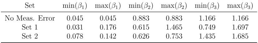
Our moment inequality estimator indicates that firms’ profit margins in export markets are between 7.8% and 14.2% and that their per-year fixed costs of exporting from Chile to the US, a distance of 5,000−6,000 miles, are about three times as large as the costs of exporting to neighboring Argentina. A comparison of the maximum likelihood estimates with our moment inequality estimates indicates that ignoring the
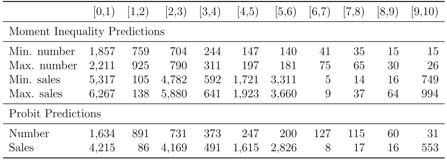
expectational error firms’ make when deciding whether to export will bias the parameter estimates in two directions: the maximum likelihood estimator (a) underpredicts the number of exporters in countries that are close to the country of origin of the firm and overpredicts entry in countries that are more distant; and (b) underpredicts the probability of entry by large firms and overpredicts this probability for small firms.
We structure the remainder of the paper as follows. In Section 2, we show that expectational error is a source of classical measurement error, and introduce a static binary choice model with both structural and expectational errors. In Section 3, we introduce both score function and revealed preference inequalities and examine the properties of these inequalities. Section 4 studies how the presence of both structural and measurement error affects the performance of estimators that neglect one of the two types of error. Section 5 generalizes the results on the benchmark model introduced in Section 2: we eliminate the parametric restrictions on the distribution of the structural error and introduce moment inequalities that identify the true value of the parameter vector without these assumptions. Section 6 describes the export decision problem and applies our inequality framework to estimate the structural parameters of a firm’s export decision. Section 7 concludes.5
2
Static Binary Choice Model
In this section, we present our statistical model. We first demonstrate that expecta-tional errors affecting agents with raexpecta-tional expectations are a special case of classical measurement error (Section 2.1). We then introduce a binary choice model that includes both structural and classical measurement error (Section 2.2). Finally, we compare our approach with alternative models in the literature (Section 2.3), and present a setting in which we carry out our simulation exercise (Section 2.4).
2.1
Expectational and Measurement Error
In this section, we demonstrate the similarities between expectational error in a ratio-nal expectations model and measurement error in a classical errors-in-variables model. Although this holds for decision problems in which the decision variable is continuous or
discrete, we show these similarities in the context of a binary choice problem to remain consistent with our statistical model of interest.
Suppose individual i faces a choice between two alternatives, j ∈ {0,1}. Firm i’s difference in payoff between alternative 1 and alternative 0 is:6
U =βE[X|J] +ν, (1)
whereJ is the information set the agent uses for her decision, E[·] denotes the expec-tation operator based on the subjective believes of the agent, and β is the parameter vector representing the agent’s preferences. The variable X may capture, for example: characteristics of alternatives that the agent imperfectly observes at the time of her decision (e.g. demand level in a market), decisions by other agents (e.g. in simultane-ous move games), or a continuation value function (e.g. dynamic discrete problems). The variable ν captures characteristics that the econometrician does not observe but that are included in J. While the parameter vector β is assumed to be constant across individuals, all the variables may vary withi. Denote the expectational error as =βX −βE[X|J] and express the difference in payoffs as:
U =βX +ν+ε, (2)
whereε =−β. Define E[·] as the expectation operator of the data generating process (DGP) forX. The DGP captures the distribution of X across individuals in the popu-lation. Under the rational expectations assumption, agents’ subjective beliefs coincide with the true DGP (i.e. E[·] = E[·]), hence: E[ε|J] = 0 and E[ε|X] 6= 0. Therefore, for any variableZ ∈ J,
E[ε|Z] = 0. (3)
An alternative way to derive the statistical model defined by equations (2) and (3) is to assume that the decision maker observes the true value of some characteristic,X∗, and selects her preferred alternative on the basis of the utility function
U =βX∗+ν, (4)
Suppose that, instead ofX∗, the econometrician observes some random variableX such
that =X−X∗, so that we can rewrite the payoff function as:
U =βX +ν+ε, (5)
whereε =−β. If we impose the classical errors-in-variables assumptions, it holds that
E[ε|X∗] = 0 and E[ε|X] 6= 0, and we define a variable Z as an instrumental variable (IV) if and only if it verifies
E[ε|Z] = 0. (6)
Equations (2) and (3) are identical to equations (5) and (6). The interpretation of the expectational error of an agent with rational expectations as a special case of the measurement error in a classical errors-in-variables model is obtained when we think of the expectation as the unobserved true covariate (i.e. E[X|J] =X∗) and of the realized future value as the observed mismeasured covariate (i.e. X).7
The difference between the rational expectations assumption and the classical errors-in-variables assumption is that the former implies a stronger orthogonality condition. While the classical errors-in-variables assumption exclusively imposesE[ε|X∗] = 0, the rational expectations assumption impliesE[ε|J] = 0, with the setJ including but not necessarily restricted to the variable X∗ =E[X|J]. For example, the interpretation of ε as expectational error implies that E[ε|ν] = 0. On the contrary, this orthogonality restriction is not imposed by the interpretation ofεas measurement error. Analogously, as long asZ∈ J, equation (3) is an implication of the rational expectations assumption. However, equation (6) is an additional restriction that is not automatically implied by the classical errors-in-variables assumption. Given that the notion of measurement error implies fewer assumptions than that of expectational error, we present our model in Section 2.2 in terms of the former and we make explicit which additional assumptions we need for our estimator to identify the true value of the parameter vectorβ.
2.2
Model
In this section, we introduce a binary choice model in which agents’ choices depend on three components: an index function that is linear in observable variables, structural error, and measurement error.
Agents’ decisions. For each individual i, we normalize the utility of one alternative to zero and express the utility of the other alternative as
U =βX∗+ν, (7)
where β ∈ Γβ ∈ RK, X∗ ∈ X∗ ∈ RK and ν ∈ R. We define a dummy variable d as d = 1{U ≥ 0}, where 1{·} is the indicator function that takes a value of 1 when {·}
is true and a value of 0 otherwise. Therefore, we can write the individual revealed preference inequality as:
(d−(1−d))·(βX∗+ν)≥0. (8)
The vector β groups the index coefficients and is defined up to a scalar normalization (possibly involving the distribution ofν). The termβX∗ is the single index determining the choice dummy,d. Both X∗ and ν belong to the information set of the agent at the time she makes a decision: (X∗, ν) ∈ J.
Measurement model. The econometrician does not observe ν and might observe X∗ with error. We denoteZ1 as the P×1 subvector of X∗ that is measured without error,
Z1 =X1∗, (9)
and X2∗ as the (K−P)×1 subvector of X∗ that may be measured with error
X =X2∗ +, (10)
where ∈ RK−P, and 0 ≤ P ≤ K.8 Once we incorporate equations (9) and (10) into equation (8), the individual-level revealed preference inequality becomes
(d−(1−d))·(β1Z1+β2X+ν+ε)≥0, (11)
with ε = −β2. In equation (11), only the vector (d, Z1, X) is observed by the econo-metrician.9 The econometrician also observes a vector of instrumental variables, Z
2 ∈
Z2 ∈ RT, T ≥ K −P. We stack both the true covariates that are observed without 8This model is consistent with either all or none of theK covariates being observed with error. 9This measurement model assumes that X and Z
error and the instruments into a single vectorZ = (Z1,Z2), Z ∈ Z ∈ RP+T.
For our moment inequality estimator, a key restriction of equation (7) is that the index function, βX∗, is linear in the unobserved true covariate, X2∗. While equation (7) assumes that this index function is also linear in the observed true covariates,X1∗, our moment inequality estimator also applies in cases in which this index function is nonlinear inX1∗.
Assumptions on error terms. We impose the following assumptions on the distribution of (ν, ε) conditional on the vector (d, X∗, Z2, X):
Assumption 1 The random variable ν is independent of the random vector (X∗, Z2);
i.e. Fν(ν|X∗, Z2) =Fν(ν).
Assumption 2 The marginal distribution function of ν is known up to a scale
parame-ter, log concave, has mean zero, and, for anyy in the support ofν, verifies the following property:
∂2E[ν|ν≥y] ∂y2 ≥0.
Assumption 3 The distribution of ε conditional on (d, X∗, Z2) has support (−∞, ∞)
and has mean zero; i.e. E[ε|d, X∗, Z2] = 0.
As in the standard binary probit or logit model, Assumption 1 imposes independence between the structural error, ν, and the true vector of covariates, X∗. Therefore, without expectational error, the error term in equation (11) is exogenous to the vector of observed covariates. Assumption 1 also imposes that the observed vector of instruments, Z2, is independent of the structural error.
logistic densities are log concave.11 As Heckman and Honor´e (1990) show, not every log concave distribution has a right-truncated expectation that is convex in the truncation point. Nevertheless, the following remark clarifies that both the normal and the logistic distribution are consistent with Assumption 2.
Remark 1 If ν ∼ N(0, σ2), for anyσ2 < ∞; orν ∼ Logistic, then ∂2E[ν|ν≥y]
∂y2 ≥0, for
any y ∈ (−∞,∞).
The proof of Remark 1 is contained in Section A.1. An implication of both Assumptions 1 and 2 is that E[ν|X∗, Z2] = 0.
Assumption 3 does not impose a parametric restriction on the distribution of the expectational error, . In contrast, as discussed in Section 4.3, estimating this binary discrete choice model using maximum-likelihood techniques would require assuming both the distribution of the measurement error conditional on the true covariates as well as the marginal distribution of these unobserved true covariates.
In addition, Assumption 3 does not require full independence between the mea-surement error and the vector of decisions, true covariates, and instruments. This is particularly important for the case in which the error ε captures expectational error and agents have rational expectations. In that case, given that (X∗, d) ∈ J and, by definition, E[ε|J] = 0, Assumption 3 can be simplified to E[ε|Z2] = 0. This condition will be satisfied as long as the econometrician defines the vector of instruments, Z2, using variables included inJ.
The data are informative about the joint density of (d, Z, X), P(d, Z, X). Any structureSa≡ {βa, fa(X|X∗, Z2)fa(Z2|X∗)fa(X∗)}is admissible as long as it verifies the restriction in Assumptions 1 to 3 and
P(d, Z, X) = Z
f(d|X∗, X;βa)fa(X|X∗, Z2)fa(Z2|X∗)fa(X∗)dX∗.
In the model described in this section, the parameter vector β is set—not point— identified, because there exists at least two admissible structuresSa1 and Sa2 such that
11A random variableyhas a log concave distribution if its density functionf
ysatisfies thatfy(λy1+ (1−λ)y2) ≥ [fy(y1)]λ [fy(y2)]1−λ, 0 ≤ λ ≤ 1, for any given values y1 and y2 in the support of
βa1 6= βa2. For a restricted version of this model, Appendix A.2 characterizes the set of structures Sa that are consistent with the joint density P(d, Z, X), and shows that these structures imply different values of the parameter vectorβ.
Although Assumptions 1 to 3 do not point-identifyβ, they have nontrivial identifi-cation power. In Section 3, we derive moment inequalities based on these assumptions; these inequalities define a set that contains the true value ofβ and is strictly contained inRK.
2.3
Related Literature
Section 2.2 introduces a binary choice model in which the observable covariates are endogenous due to the existence of classical errors-in-variables. Our paper is not the first to study identification of index-function parameters in a binary choice model with endogenous observable covariates. But we are, to our knowledge, the first to examine the identifying properties of Assumptions 1 to 3 in an economic model that contains two distinct errors with different economic interpretation.
There are three alternative models that build on conditional independence assump-tions to identify the parameters of binary choice models with endogenous regressors: (1) the IV model of Chesher (2010) and Chesher (2011); (2) the triangular system model that motivates the use of control function methods; and, (3) the special regressor ap-proach.
As Blundell and Powell (2003) show, even when the econometrician observes an excluded variable that is independent of the error term in the random utility function, semi-parametric and non-parametric binary response models are generally not point identified. Chesher (2010) shows that this result holds even if we impose parametric restrictions both on the random utility function and on the marginal distribution of the error term. Chesher (2010) provides the inequalities that sharply define the identified set under the assumption that the econometrician observes a excluded variable that is independent of the error term (i.e. fully independent instrument). While Chesher (2010) focuses on the case in which the endogenous variable is continuous, Chesher (2011) performs an analogous exercise for the case in which it is discrete.12 Following our notation, Chesher (2010) and Chesher (2011) assume that (ν+ε)|Z ∼(ν+ε).
Our model is stricter than the one proposed in Chesher (2010) in that we formally
define the error term as the sum of two different unobserved components: structural error, ν, and expectational error, ; we only allow for endogeneity that is due to ex-pectational error. However, our model can be viewed as more flexible than that in Chesher (2010) because our identification strategy does not assume that the aggregate error term, (ν +), is fully independent of the instrument vector,Z2. We only need to impose mean independence between this instrument and . This weaker independence assumption of our statistical model matches the assumptions common to economic models of agents with rational expectations.13
The triangular system control function model is attractive because, under certain conditions, point identifies the parameters of interest. In particular, Blundell and Pow-ell (2004) obtain point identification by applying a control-function approach. This approach assumes that the endogenous variables are determined by an equation X = h(Z, e) such that there is a one-to-one mapping from the latent variables, e, to the endogenous variables, X, at each value of the instrument vector, Z.14 Using the notation introduced in Section 2.2, the latent variable e is assumed to verify: (ν +ε)|X, Z ∼ (ν +ε)|X, e ∼ (ν +ε)|e. In contrast, our model is a single-equation model: there is no specification of any structural equation that would imply that the error term (ν+ε) is independent of the endogenous regressor X, conditional on some latent variable, e.15
The special regressor approach assumes that the aggregate unobservable component, (ν+), is distributed independently of a continuously distributed explanatory variable (i.e. special regressor) and impose a particular index restriction (Lewbel (2000)). This model is point identified only if the special regressor has large support. In an application in which the only source of endogeneity is expectational error, this approach implies that one covariate, the special regressor with large support, is measured without error.16 Our statistical model allows all the regressors to contain expectational error.
13The only type of independence that the rational expectations assumption imposes on the definition of the expectational error is mean independence between this error and any variable contained in the information set of the agent.
14This restriction rules out cases in which there are discrete endogenous variables. In our case, we allow for discrete endogenous variables as long as the measurement error can verify the restriction in Assumption 3.
15Other papers that explore the use of control function methods for the identification of binary choice models in semi- and non-parametric settings are Blundell and Powell (2003), Chesher (2003), Chesher (2005), Chesher (2007), Vytlacil and Yildiz (2007), Florens et al. (2008), Imbens and Newey (2009), and Shaikh and Vytlacil (2011).
2.4
Simulation Exercise: Setting
We now introduce a simple setting that we will use in Sections 3 and 4 to illustrate the properties of our moment inequality estimator. The simulated data is generated by a structure in which
U =β1X1∗+β2X2∗+β3X3∗+ν, (12) withβ = (0.5,0.5,0.25). The error ν is distributed normally and independently ofX∗: ν|X∗ vN(0,2).17 We assume that X∗
1 andX ∗
3 are measured without error: {Z1, Z3}=
{X1∗, X3∗}. On the other hand, the variable X2∗ is measured with error: X2 =X2∗ + x, with x distributed normally and independently of (X∗, ν): x|(X∗, ν)vN(0,0.4). We also repeat the estimation for values ofσ2x between 0.2 and 1.8, in order to study how the
properties of the different estimators change as the variance of the expectational error increases. Finally, we generate our instrumental variable,Z2, as a second measurement ofX2∗: Z2 = X2∗ +z, withz distributed normally and independently from (X
∗, ν, x):
z|(X∗, ν, x)vN(0,0.04).18
3
Moment Inequalities
In this section, we introduce two different types of moment inequalities that (partially) identify the vector β of index coefficients under the assumptions of the static model described in Section 2.2. Section 3.1 derives both types of inequalities conditional on the vector of instruments, Z. Section 3.2 converts these conditional moments into unconditional moments. In Section 3.3, we illustrate the identification power of these unconditional moment inequalities in our simulation exercise.
3.1
Conditional Moment Inequalities
For any given value of the instrument vectorZ, we derive two different types of inequal-ities: score function moment inequalities and revealed preference moment inequalities. 17We assume thatν is the difference in the structural error between alternative 1 and alternative 0. Withν1|X∗vN(0,1),ν0|X∗vN(0,1), and both independent from each other,ν|X∗= (ν1−ν0)|X∗v
N(0,2).
3.1.1 Conditional Score Function Moment Inequalities
For anyz ∈ Z, we define the conditional score function moment inequality as
Ms(z;β) = E "
m−s(d, Z1, X;β) m+
s(d, Z1, X;β)
Z =z #
≥0,
where the two moment functions are defined as
m−s(d, Z1, X;β) =d
Fν −(β1Z1+β2X)
1−Fν −(β1Z1+β2X)
−(1−d), (13a)
m+s(d, Z1, X;β) = (1−d)
1−Fν −(β1Z1+β2X)
Fν −(β1Z1+β2X)
−d. (13b)
While m+
s is increasing in β1Z1 +β2X, the opposite is true for m−s. We derive these inequalities by differentiating the log probability of d= 1 -hence, the label score func-tion inequality.19 We use M
s(ZM;β) to group the conditional moment inequalities corresponding to the set of values of z contained in the vector ZM: M
s(ZM;β) =
{Ms(z;β); for all z ∈ ZM}. We denote the identified set defined by these inequalities as Ω(Ms,ZM) = {β ∈ Γβ : Ms(z;β) ≥ 0 for allz ∈ ZM}. The following theorem contains the properties of the set Ω(Ms,ZM). We use β∗ to denote the true value of β.
Theorem 1 Properties of Ω(Ms,ZM).
1. If Assumptions 1, 2 and 3 hold, then β∗ ∈Ω(Ms,ZM),for anyZM ⊆ Z and any β∗ ∈ Γβ.
2. If Assumptions 1 and 2 hold and X2∗ =X =Z2, then β∗ = Ω(Ms,ZM), for any
ZM ⊆ Z such that the rank of the K ·M matrix (z1, . . . , zM) ∈ ZM is larger than K, and any β∗ ∈ Γβ.
3. If Assumptions 1, 2 and 3 hold andσ¯¯2
ε ≥σ¯ε2, thenΩ(Ms,ZM|σ¯ε2)⊆Ω(Ms,ZM|σ¯¯ε2), for any ZM ⊆ Z.
The proofs of the three properties of Ω(Ms,ZM) in Theorem 1 are contained in Sections A.3, A.4, and A.5, respectively.20 The first property indicates that, if Assumptions 1, 2
19We describe its derivation in detail in Section A.3.
and 3 hold, then the score function inequalities contain the true value of the parameter vector, for anyβ∗ and any valid set of instruments. In general, the set Ω(Ms,ZM) will also contain values ofβ other than its true value. However, as the second property in Theorem 1 states, in the particular case in which there is no expectational error (i.e. X2∗ =X) and we use the observed vector of choice characteristics as instruments (i.e. Z2 = X), the identified set defined by the score function inequalities is a singleton, containing only the true value of the parameter vector. Finally, in those cases in which there is measurement error (i.e. X2∗6=X) and, therefore, we use a vector of instruments different from the observed covariates (i.e. Z2 6=X), the third property in Theorem 1 states that the set Ω(Ms,ZM) increases monotonically in the variance of the expectational error. Specifically, every value of the vectorβ contained in the identified set that corresponds to a given value of the variance of the measurement error will also be contained in the identified set generated by a larger variance.
Computing the moments in equation (13) is no harder than evaluating the likelihood function for a binary choice model that assumes there is no expectational error. We describe the formation of the moments below.
3.1.2 Conditional Revealed Preference Inequalities
For anyz ∈ Z, we define the conditional revealed preference moment inequality as
Mr(z;β) =E "
m−r(d, Z1, X;β) m+
r(d, Z1, X;β)
Z =z #
≥0,
where the two moment functions are defined as
m−r(d, Z1, X;β) =−(1−d)(β1Z1+β2X) +dE
ν|ν≥ −(β1Z1+β2X), Z1, X
, (14a)
m+r(d, Z1, X;β) =d(β1Z1+β2X) + (1−d)E
−ν| −ν≥β1Z1+β2X, Z1, X
. (14b)
While m+
r is increasing in the index β1Z1 +β2X, the opposite is true for m−r. We derive these inequalities from the individual revealed preference inequality of the version of the model described in Section 2.2 that does not contain expectational error (see equation (8)) –hence, the labelrevealed preference inequality.21 Analogously to the case of the score function inequality, we define Mr(ZM;β) = {Mr(z;β); for all z ∈ ZM}
that the log concavity of the distribution ofνis sufficient to guarantee that bothFν(·)/(1−Fν(·)) and (1−Fν(·))/Fν(·) are convex.
and Ω(Mr,ZM) = {β ∈ Γβ : Mr(z;β) ≥ 0 for all z ∈ ZM}. The following theorem contains the properties of the set Ω(Mr,ZM).
Theorem 2 Properties of Ω(Mr,ZM).
1. If Assumptions 1, 2 and 3 hold, then β∗ ∈ Ω(Mr,ZM), for any ZM ⊆ Z and any β∗ ∈ Γβ.
2. If Assumptions 1 and 2 hold and X2∗ = X = Z2, then ∃ β ∈ Γβ such that β 6= β∗ and β ∈Ω(Mr,ZM), for any ZM ⊆ Z and any β∗ ∈ Γβ.
3. If Assumptions 1, 2 and 3 hold andσ¯¯ε2 ≥σ¯ε2, thenΩ(Mr,ZM|¯σ2ε)⊆Ω(Mr,ZM|σ¯¯ε2), for any ZM ⊆ Z.
The proof of the three properties of Ω(Mr,ZM) in Theorem 2 are contained in Sections A.6, A.7, and A.8, respectively. The first property indicates that, if Assumptions 1, 2 and 3 hold, then Ω(Mr,ZM) contains the true value of the parameter vector, for any β∗ and instrument vector. As Theorem 2.2 indicates, the set Ω(Mr,ZM) will generally also contain values of β other than its true value. In fact, contrary to the case of the score function inequalities, the set identified by the revealed preference inequalities is never a singleton. Even in cases in which the econometrician assumes that the observed covariate, X, is identical to the true covariate, X2∗, and, therefore, uses X as an instrument, it is still true that the set Ω(Mr,ZM) will contain values of the parameter vector that are different from β∗. A comparison of Theorem 1.2 and Theorem 2.2 leads to the conclusion that, for any ZM, if X∗
2 = X = Z2, then Ω(Ms, z|σε2 = 0) ⊂ Ω(Mr, z|σε2 = 0). This does not imply that, for any ZM, the inequalitiesMr(ZM;β) are irrelevant once we include the inequalitiesMs(ZM;β). On the contrary, Theorems 1 and 2 provide little guidance on how Ω(Ms,ZM) compares to Ω(Mr,ZM) when the variance of the expectational error is different from zero. The third property in Theorem 2 is analogous to the third property in Theorem 1.
Computing the moment inequalities in equation (14) requires evaluating the right-truncated expectation ofν at different values in its support. For both probit and logit models, the right-truncated expectation of the structural error may be computed using standard statistical packages.22
22If ν ∼N(0, σ2), then E[ν|ν ≥y] = (σφ(y/σ))/(1−Φ(y/σ)). Ifν ∼Logistic, thenE[ν|ν ≥y] =
3.2
Unconditional Moment Inequalities
The moment inequalities described in equations (13) and (14) condition on particular values of the instrument vector, Z. In empirical applications in which at least one of the variables in the vector Z is continuous, the sample analogue of these moment inequalities will likely involve an average over very few observations (if any). Therefore, for estimation, it will be more useful to work with unconditional moment inequalities.
Each of the unconditional moment inequalities is defined by aninstrument function. Here, we propose a particular set of instrument functions.23 We identify each of these functions by a K ×1 vector q of 0s and 1s. We group all these vectorsq into a matrix Qthat forms the standard basis in RK. For eachq, we define an instrument function:
Ψq(Z) =
K Y
k=1
(1{Zk ≥0})qk(1{Zk<0})1−qk;qk ∈ {0,1}, k= 1, . . . , K , (15)
whereZk is the kth element of Z and qk is the kth element of q.24
Using the instrument functions Ψq,q ∈Q, we defineQunconditional score function moment inequalities and Q unconditional revealed preference inequalities. We denote the unconditional score function inequality defined by the instrument Ψq as Mqs(β). Analogously, we denote the corresponding revealed preference inequality as Mq
r(β).
3.2.1 Unconditional Score Function Moment Inequalities
For each q ∈ Q, the resulting unconditional score function moment inequality is
Mq
s(β) = E h
Ψq(Z)·m+s(d, Z1, X;β) + Ψq(−Z)·m−s(d, Z1, X;β) i
≥0. (16)
We group theQunconditional score function moment inequalities into the vectorMs(β) and define an identified set for this group of inequalities: Ω(Ms) = {β ∈Γβ :Ms(β)≥
23The unconditional moment inequalities proposed here generate a larger identified set than that defined by the conditional moments described in Section 3.1. The main advantage of the moments proposed here is its computational simplicity, while they still generate a bounded set. Papers that define unconditional moments that imply no loss of information with respect to their conditional counterpart are Amstrong (2012) and Andrews and Shi (2013). The instrument functions used in these papers are computationally very intensive in our setting.
0}. The following theorem contains the properties of the set Ω(Ms).
Theorem 3 Properties of Ω(Ms).
1. If Assumptions 1, 2 and 3 hold, then β∗ ∈Ω(Ms), for any β∗ ∈ Γβ. 2. If Assumptions 1 and 2 hold, X2∗ =X =Z2, and, for every q ∈ Q,
E
"
Ψq(Z) + Ψq(−Z) #
6
= 0, (17)
then β∗ = Ω(Ms).
3. If Assumptions 1, 2 and 3 hold and σ¯¯2
ε ≥ σ¯2ε, then Ω(Ms|σ¯ε2)⊆Ω(Ms|σ¯¯2ε). 4. If Assumptions 1, 2 and 3 hold and, for every β ∈ Γβ and q ∈ Q,
∂Mq s(β) ∂βk
>0, if qk = 1, (18a) ∂Mq
s(β) ∂βk
<0, if qk = 0, (18b)
then Ω(Ms) is bounded and closed.
5. If Assumptions 1, 2 and 3 hold, then Ω(Ms) is convex.
The first property indicates that the true value of the parameter vector is contained in the identified set defined by the Q unconditional score function moment inequalities in equation (16). This comes immediately from Theorem 1.1 and the fact that, for every q ∈ Q, we can rewrite Mq
s(β) as
Mq
s(β) =E h
Ψq(Z)·E
m+s(d, Z1, X;β)
Z+ Ψq(−Z)·E
m−s(d, Z1, X;β)
Zi. (19)
For every Z ∈ Z, Em+s(d, Z1, X;β∗)Z ≥ 0 and Em−s(d, Z1, X;β∗)Z ≥ 0. There-fore,Mq
s(β∗)≥0.
the particular case in which there is no expectational error and we use the observed covariate X as an instrument, Z2, then the only value of the parameter vector β that is consistent with theseQ unconditional inequalities is the true value of the parameter vector,β∗.
In cases in whichX 6= X2∗, the identified set Ω(Ms) will generally contain values of the parameter vectorβ other than its true value. Theorem 3.3 indicates that the set of values that are included in Ω(Ms) increases in the variance of the expectational error, σ2
ε. This is a direct consequence of Theorem 1.3 and the unconditional inequalities being weighted averages of the conditional moment inequalities across different values of Z (equation (19)).
Equation (18) in Theorem 3.4 establishes some conditions under which the Q un-conditional score function moment inequalities imply that the identified set is bounded. That is both, for everyβk,k = 1, . . . , K, both +∞and −∞are excluded from Ω(Ms). Equation (18) requires that the partial derivative of each moment function, Mq
s(β), with respect to each element of the parameter vector, βk, is determined by the instru-ment function in equation (15). In order for equation (18) to hold, the correlation between the endogenous variable X, and its instrument, Z2, must be sufficiently large. Therefore, this property of the identified set Ω(Ms) depends on the instruments being sufficiently strong. The proof of Theorem 3.4 is contained in Section A.10.
Finally, Theorem 3.5 establishes convexity of the set Ω(Ms). Convexity is an im-portant property for for inference in partially-identified models (see Beresteanu and Molinari (2008), Kaido and Santos (2011), and references therein). The proof of Theo-rem 3.5 is contained in Section A.11.
3.2.2 Unconditional Revealed Preference Moment Inequalities
For each q ∈ Q, the resulting unconditional revealed preference moment inequality is
Mq
r(β) = E h
Ψq(Z)·m+r(d, Z1, X;β) + Ψq(−Z)·m−r(d, Z1, X;β) i
≥0. (20)
We group theQ unconditional revealed preference moment inequalities into the vector
Mr(β) and define an identified set for this group of inequalities: Ω(Mr) = {β ∈ Γβ :
Mr(β)≥0}. The following theorem contains the properties of the set Ω(Mr).
Theorem 4 Properties of Ω(Mr).
2. If Assumptions 1 and 2 hold and X2∗ = X = Z2, then ∃ β ∈ Γβ such that β 6= β∗ and β ∈Ω(Mr), for any β∗ ∈ Γβ and β∗ 6= 0.
3. If Assumptions 1, 2 and 3 hold and σ¯¯2
ε ≥ σ¯2ε, then Ω(Mr|σ¯ε2)⊆Ω(Mr|σ¯¯ε2). 4. If Assumptions 1, 2 and 3 hold and, for every β ∈ Γβ and q ∈ Q,
∂Mq r(β) ∂βk
>0, if qk = 1, (21a) ∂Mq
r(β) ∂βk
<0, if qk = 0, (21b)
then Ω(Mr) is bounded and closed.
5. If Assumptions 1, 2 and 3 hold, then Ω(Mr) is convex.
Properties 1, 3, 4, and 5 are identical to those described in Theorem 3 for the case of the set Ω(Ms). We refer to the comments in Section 3.2.1 and proofs in Sections A.10 and A.11.
Among the list of characteristics listed in Theorems 3 and 4, the only difference between the sets Ω(Ms) and Ω(Mr) is the identification properties of these two sets in the case in which the econometrician assumes that there is no expectational error in covariates, X2∗ = X, and, accordingly, uses such observed covariates as arguments of the instrument function. While the set defined by the unconditional score function inequalities collapses to a singleton containing onlyβ∗(see Theorem 3.4), the set defined by the unconditional revealed preference inequalities will include values of the parameter vector other than its true value (see Theorem 4.4). This is an immediate consequence of Theorem 2.2 and that each momentMq
r(β) is a weighted average of a particular set of conditional moments, Mr(z;β).
3.2.3 Combining Score Function and Revealed Preference Inequalities
Theorem 5 Properties of Ω(M).
1. If Assumptions 1, 2 and 3 hold, then β∗ ∈Ω(M), for any β∗ ∈ Γβ. 2. If Assumptions 1 and 2 hold, X2∗ =X =Z2, and, for every q ∈ Q,
E
"
Ψq(Z) + Ψq(−Z) #
6
= 0, (22)
then β∗ = Ω(M).
3. If Assumptions 1, 2 and 3 hold and σ¯¯2
ε ≥ σ¯2ε, then Ω(M|σ¯ε2)⊆Ω(M|¯¯σε2). 4. If Assumptions 1, 2 and 3 hold and, for every β ∈ Γβ and q ∈ Q,
max
∂Mq s(β) ∂βk
,∂M q r(β) ∂βk
>0, if qk = 1, (23a)
min
∂Mq s(β) ∂βk
,∂M q r(β) ∂βk
<0, if qk = 0, (23b)
then Ω(M) is bounded and closed.
5. If Assumptions 1, 2 and 3 hold, then Ω(M) is convex.
Theorem 5 is a direct implication of Theorems 3 and 4 and the vectorM(β) including both the unconditional score and revealed preference inequalities.
Ω(M) to be closed and bounded. Finally, Theorem 5.5 is just an immediate implication of all the unconditional score function and revealed preference inequalities being convex.
3.3
Simulation Exercise
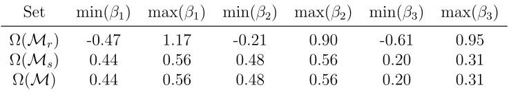
Table 1 contains the identified sets Ω(Ms), Ω(Mr) and Ω(M) for our simulation exer-cise. For all three sets, we assume that the econometrician knows the exact distribution of the structural error. We compute the maximum and minimum value of each of the three parameters that belongs to the three identified sets.
Table 1: Identified Set
Set min(β1) max(β1) min(β2) max(β2) min(β3) max(β3) Ω(Mr) -0.47 1.17 -0.21 0.90 -0.61 0.95
Ω(Ms) 0.44 0.56 0.48 0.56 0.20 0.31
Ω(M) 0.44 0.56 0.48 0.56 0.20 0.31
In Table 1, the true value of the parameter vector, (0.5,0.5,0.25), lies within the smallest square circumscribing each of the three identified sets. The set Ω(Mr) is much larger than the set Ω(Ms); Ω(M) and Ω(Ms) are virtually identical. For example, the set Ω(Mr) indicates that the true value of β1 lies on the interval (−0.47, 1.17), Ω(Ms) and Ω(M) indicate that it lies on the interval (0.44,0.56). In sum, the revealed preference moment inequalities are far less informative about the true value of the parameter vector than the score function inequalities. We illustrate the relative size of these two identified sets in a 2-dimensional space in Figure 1.25
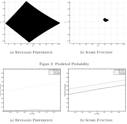
We illustrate the predicted probabilities in Figure 2. In this figure, we report both the true probability as well as the minimum and maximum predicted probability from the model, using the “true” covariates for a particular agent and the set of parameter values contained in the identified sets Ω(Ms), Ω(Mr) and Ω(M). In Figure 2, we fix (X1∗, X3∗) to arbitrary values and plot the minimum, maximum, and the true probabili-ties in our simulation for a range of values of theX2∗ covariate. Combining the revealed preference and score function moments yields a range of predicted probabilities that closely follows the true probabilities.
Figure 1: Identified Set
0 0.1 0.2 0.3 0.4 0.5 0.6 0.7 0.8
−0.4 −0.2 0 0.2 0.4 0.6 0.8 2 3
Identified Set for Sample Dataset in Monte Carlo Exercise 1=0.5, Using only Revealed Preference Moments
(a)Revealed Preference
0 0.1 0.2 0.3 0.4 0.5 0.6 0.7 0.8
−0.4 −0.2 0 0.2 0.4 0.6 0.8 2 3
Identified Set for Sample Dataset in Monte Carlo Exercise
1=0.5, Using only Score Function Moments
(b) Score Function
Figure 2: Predicted Probability
−0.6 −0.4 −0.2 0 0.2 0.4 0.6 0 0.1 0.2 0.3 0.4 0.5 0.6 0.7 0.8 0.9 1
X2 range
Predicted Probabilities
Predicted Probabilities for Difference Ranges of X2
Moment Inequalities from Dickstein Morales (2013), Revealed Preference Moments Only Uses Observed Z2 as an Instrument for X2
Min Prob Max Prob True Prob
(a)Revealed Preference
−0.6 −0.4 −0.2 0 0.2 0.4 0.6
0 0.1 0.2 0.3 0.4 0.5 0.6 0.7 0.8 0.9 1
X2 range
Predicted Probabilities
Predicted Probabilities for Difference Ranges of X2 Moment Inequalities from Dickstein Morales (2013), All Moments
Uses Observed Z2 as an Instrument for X2
Min Prob Max Prob True Prob
(b) Score Function
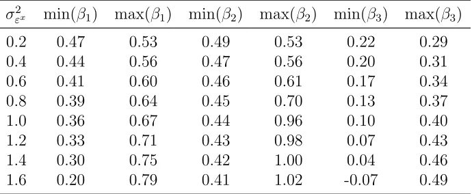
Property 3 in Theorem 5 states that the size of the identified set Ω(M) increases as the variance of the expectational error increases. We show this in Table 2. The bounds in this table use both the score function and the revealed preference inequalities. In order to compute each row of this table, we have generated samples of 100,000 observations using a statistical model identical to that described in Section 2.4, but with the variance of the expectational error,σ2x, set to equal the value indicated in the
Table 2: Identified Set for Different Variances
σ2
εx min(β1) max(β1) min(β2) max(β2) min(β3) max(β3)
0.2 0.47 0.53 0.49 0.53 0.22 0.29
0.4 0.44 0.56 0.47 0.56 0.20 0.31
0.6 0.41 0.60 0.46 0.61 0.17 0.34
0.8 0.39 0.64 0.45 0.70 0.13 0.37
1.0 0.36 0.67 0.44 0.96 0.10 0.40
1.2 0.33 0.71 0.43 0.98 0.07 0.43
1.4 0.30 0.75 0.42 1.00 0.04 0.46
1.6 0.20 0.79 0.41 1.02 -0.07 0.49
4
Potential Misspecification of the Model
In spite of the empirical relevance of the statistical model described in Section 2.2, to our knowledge, the previous literature does not provide a valid estimator for such a model. In this section we consider three possible deviations from the model described in Section 2.2 that appear in the literature. These alternative specifications substitute one of the three assumptions of our binary choice model for a more restrictive alter-native assumption. These additional restrictions lead to a different identification and estimation approach from the moment inequality estimator introduced in Section 3. In this section, we explore the properties of these alternative procedures as ways to iden-tify the parameter vector β for the binary choice model described in Section 2.2. We show that, if the model described in Section 2.2 is the true model, assuming a simplified version of it may lead to large biases in the identification of the index coefficients and in the prediction of the choice probabilities.
4.1
Invalid Instrument
Even if the researcher believes that the statistical model described in Section 2.2 is adequate to capture the main features of her empirical setting, three issues may com-plicate the application of the inequality estimator described in Section 3. First, there may be no observed vector of excluded variables, Z2, in the dataset available. Second, even if such a vector of excluded variables exist, the correlation between these vari-ables and the mismeasured vector of covariates, X, might be so small such that the resulting identified set Ω(M) is unbounded (i.e. the restrictions in equation (23) fail to hold). Finally, there may be cases in which the econometrician wrongly assumes that X2 has no expectational error (i.e. assumes that X2∗ = X). In these three cases, the econometrician may decide to include the endogenous variableX as an argument of the instrument function,{Ψq;q = 1, . . . , Q}, in place ofZ2. Implicitly, the econometrician substitutes Assumption 3 by the following alternative assumption:
Assumption 3(b) The distribution of ε conditional on (X, ν) has support equal to
(−∞, ∞) and expectation equal to 0: E[ε|X, ν] = 0.
Assumption 3(b) imposes that the expectational error is mean independent of the ob-served covariate instead of being mean independent of true (unobob-served) covariate. Given this assumption, one can define an identified set that contains β∗ without the instrument vector Z. We can write a vector instrument functions {Ψq; q = 1, . . . , Q}
identical to that in equation (15) that takes the vector X as their argument. The resulting moment inequalities are:
Mq
s(β) =E h
Ψq((Z1, X))·m+s(d, Z1, X;β) + Ψq((−Z1,−X))·m−s(d, Z1, X;β) i
≥0,
Mq
r(β) =E h
Ψq((Z1, X))·m+r(d, Z1, X;β) + Ψq((−Z1,−X))·m−r(d, Z1, X;β) i
≥0.
for q = {1, . . . , Q}. We use M(β) to denote the 2 ·Q moment inequalities whose instrument function depends on the observed vector of covariates (Z1, X) (contrary to
M(β), which identifies the inequalities described in Section 3 and whose instrument function depends on Z = (Z1, Z2)). We denote Ω(M) as the set of values of β ∈ Γβ that are consistent with the moments identified by M(β). Analogously, we can define Ω(Ms) and Ω(Mr).
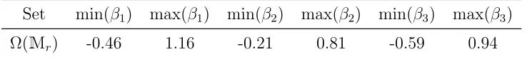
Assumption 3(b), then the non-zero correlation between the expectational error affect-ing X and the instrument vector, {Ψq((X, Z));q = 1, . . . , Q}, will affect the moments in the vector M(β). We use our simulation to explore the properties of the identified set, Ω(M), when Assumption 3 holds.
Table 3: Identified Set
Set min(β1) max(β1) min(β2) max(β2) min(β3) max(β3) Ω(Mr) -0.46 1.16 -0.21 0.81 -0.59 0.94
The results from the simulation appear in Table 3. In this example, Ω(Ms) = Ω(M) =∅. At least two of the score function moments cross each other and, therefore, there is no value of the parameter vector that satisfies all score function moments. This shows that, given the statistical model described in Section 2.2, the true value of the parameter vector is not consistent with the vector of moments M(β).26 In sum, if Assumption 3 holds instead of Assumption 3(b), we cannot guarantee that Ω(Ms) or Ω(Mr) contain the true value of the parameterβ.
4.2
No Structural Error
The previous empirical literature that applies moment inequalities to identify the pa-rameters of a discrete choice model often explicitly or implicitly rules out an idiosyn-cratic structural error. That is, the econometrician assumes that the unobserved com-ponents of the agent’s utility function are identical across choices: ν = 0. Examples of empirical applications using moment inequalities that impose this assumption in-clude Ho (2009), Pakes (2010), Pakes et al. (2011), Holmes (2011), and Morales et al. (2011).27
26We also find that β∗ ∈ Ω(M
r). However, Ω(Mr) is smaller than Ω(Mr). The fact that Ω(Mr) contains the true value of the parameter vector is due to the weak identification power of the revealed preference moment inequalities. That is, the revealed preference inequalities admit a wide range ofβ
values in the identified set.
In order to derive score function and revealed preference moment inequalities under the assumption of no structural error, we work with a statistical model that is equiv-alent to that in Section 2.2, except that we replace Assumption 2 with the following alternative assumption:
Assumption 2(b) The marginal distribution function of ν has a degenerate
distribu-tion at ν = 0.
If Assumptions 1, 2(b) and 3 hold, then the score function moment inequality (equation (16)) has no identification power.28 As a consequence, for eachq∈Q, the only inequality with identification power is the following revealed preference inequality:
Mqr(β) =Eh−Ψq(Z)(1−d)(β1Z1+β2X) + Ψq(−Z)d(β1Z1+β2X) i
≥0. (24)
and the identified set defined by theseQmoment inequalities is Ω(Mr). If Assumptions 1, 2(b) and 3 hold, then the identified set Ω(Mr) contains the true value of the parameter vector and is convex, bounded, and closed.29
We use our simulation to explore the properties of the identified set Ω(Mr) in settings in which Assumption 2 holds and Assumption 2(b) does not. That is, we examine the coverage properties of the set Ω(Mr) in settings in which the structural error varies across choices but the econometrician wrongly assumes that it is identical across choices. Note that, for everyq ∈ Q, we can write Mq
r(β) = Mqr(β) +γq(β) and, for every value of β ∈ Γβ and every q ∈ Q, γq(β) ≥ 0.30 Therefore, Ω(Mr) ⊂ Ω(Mr) and we cannot prove that, if Assumptions 1, 2 and 3 hold (and Assumption 2(b) does not) β∗ is contained in Ω(Mr). In words, when we wrongly assume that there is no structural error, the identified set defined by the resulting moment inequalities is biased inwards. This can lead to a false sense of precision. If Assumption 2(b) does not hold,
discrete choice problems is thus limited. In the application in Ciliberto and Tamer (2009), the moment inequalities estimator allows a structural error but contains no expectational error. We consider the effect of incorrectly assuming that there is no expectational error in Section 4.3.
28Proof in Section A.12. 29More precisely, the set Ω(M
r) is a K-dimensional cube. The “flat faces” in the boundary of the identified set is a direct implication of the linearity of the moment inequalities in the parameter vector
β (see Kaido and Santos (2011)).
30The functionγq(β) is a weighted average of truncated expectations and works as a structural error correction term. Its exact expression is:
EhΨq(Z)dE[ν|ν≥ −(β1Z1+β2X), Z1, X] + Ψq(−Z)(1−d)E[−ν| −ν≥β1Z1+β2X, Z1, X]
the identified set Ω(Mr) may be so small that it may fail to contain the true value of the parameter vector. The results from the simulation exercise demonstrate this possibility: Table 4 shows that Ω(Mr) is much smaller than Ω(Mr). While the resulting identified set still contains the true value of β3, this is not true for the parameter β2. The true value ofβ2 is 0.5, while the identified set found for this parameter is (−0.11,0.24).31
Table 4: Identified Set
Set min(β1) max(β1) min(β2) max(β2) min(β3) max(β3)
Ω(Mr) 0.50 0.50 -0.11 0.24 -0.21 0.28
The absence of structural error makes the resulting model fully deterministic. There-fore, for any given vector X∗, the predicted choice probability for any alternative is either 1 or 0.
4.3
No Expectational Error
Finally, we consider the potential misspecification in which the econometrician ignores expectational error. To our knowledge, no paper allows for classical errors-in-variables in a binary choice model.32 The standard binary choice model allows for a single error term and assumes that its distribution is known up to a finite vector of parameters. Formally, the standard model estimated in the binary choice literature assumes d·
(βX +η)≥ 0, η|X ∼ fη(η|X;ρ), where the distribution of the error term, fη(η|X;ρ), is unknown up to the parameterρ. The probability that an individual with observable characteristicsX selects choice j is equal to:
P(d = 1|X) = Z
η
1{η ≥ −βX}dFη(η|X;ρ). (25)
Only under very strong assumptions would this choice probability arise from a model that allows both for structural and measurement error, as in the model introduced in Section 2.2. In order to facilitate the comparison, assume the statistical model
31When we assume that the structural error equals 0, we first must define an alternative normaliza-tion by scale for the parameterβ. For comparison purposes, we set the correct scale by fixingβ1 to be equal to its true value, 0.5.
described in equations (7) to (11) and impose the following distributional assumptions: ν ∼ Fν(ν|X∗;ρ1), and ε ∼ Fε(ε|X∗;ρ2). The resulting conditional choice probabilities are
P(d= 1|X) = Z
x∗
hZ
ν
1{ν ≥ −βX∗}dFν(ν|X∗;ρ1) i
dFx∗(X∗|X;ρ2) (26)
where computing Fx∗(X∗|X;ρ2) requires knowledge of Fε(ε|X∗;ρ2) and the marginal
distribution of the vector of unobserved covariates, Fx∗(X∗). Therefore, in the model
in Section 2.2, in order to account for the measurement error in a maximum likelihood setting, one must make parametric assumptions on two additional distributions: (a) the distribution of the measurement error conditional on the true covariates, and, (b) the marginal distribution of the true covariates.33
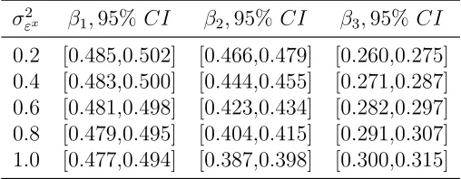
The results of the simulation exercise show the asymptotic bias that would arise from ignoring expectational error. Table 5 presents the ML estimates for data gener-ated following the statistical model described in Section 2.4, with the variance of the measurement error, σ2
x, set equal to the value indicated in the first column. In order
to make the results comparable, we rescale the ML estimates so that the estimates presented in every row are subject to the same normalization. The results show that as the variance of the measurement error inX2 increases, the ML estimate of β2 is biased downward and the ML estimate of β3 has an upward bias.
Consider the particular case in which the variance of the expectational error is set to 0.2 (10% of the variance of the structural error). As shown in Table 5, at 0.4, the 95% confidence interval for β2 and β3 do not contain the true value of the parameter vector. Thus, even a relatively small variance of the measurement error might generate significant bias in the ML estimator.
33By redefining η as ε + ν, one might be tempted to consider equation (25) as the reduced form analogue of equation (26). To do so, however, requires the researcher to impose strong independence assumptions on Fν(ν|X∗;ρ1) and Fε(ε|X;ρ2). As an example, if one assumes that Fν(ν|X∗;ρ1) =
Fν(ν;ρ1) andFε(ε|X;ρ2) = Fε(ε;ρ2), then equation (26) becomes
P(d= 1|Xi) =
Z
ν+ε
1{ν+ε≥ −βX∗}dFν(ν+ε; (ρ1, ρ2)), (27)
Table 5: Maximum Likelihood with Measurement Error
σ2
εx β1,95% CI β2,95% CI β3,95% CI 0.2 [0.485,0.502] [0.466,0.479] [0.260,0.275] 0.4 [0.483,0.500] [0.444,0.455] [0.271,0.287] 0.6 [0.481,0.498] [0.423,0.434] [0.282,0.297] 0.8 [0.479,0.495] [0.404,0.415] [0.291,0.307] 1.0 [0.477,0.494] [0.387,0.398] [0.300,0.315]
5
Nonparametric Assumptions on Structural Errors
All the moment inequalities derived in Section 3 rely on the assumption that that the econometrician knows the marginal distribution of the structural error up to a scale parameter. In this section, we derive moment inequalities that do not require the econometrician to specify a distribution for ν. These moment inequalities hold at the true value of the parameter vector as long as Assumptions 1 and 3 hold and the structural error has zero mean. The lack of parametric assumptions on the distribution ofνimpedes the derivation of the score function inequalities. However, we are still able to derive the revealed preference inequalities.
5.1
Revealed Preference Inequalities
If the econometrician does not assume a particular distribution function forν, then she cannot compute the terms E[ν|ν ≥ −(β1Z1 +β2X), Z1, X] and E[−ν| −ν ≥ β1Z1 + β2X, Z1, X] in equation (14). Nevertheless, we can still find an inequality that will be satisfied at the true (normalized) value of the parameter vector. For every instrument function Ψq, q = 1, . . . , Q (see equation (15)), we define the following inequality:
Mqr(β) =EhΨq(Z)·m+r(d, Z1, X;β) + Ψq(−Z)·m−r(d, Z1, X;β) i
≥0, (28)
with
m−r(d, Z1, X;β) = (1−d)(−(β1Z1+β2X)) +E
ν1{ν ≥0}
, (29a)
m+r(d, Z1, X;β) = d(β1Z1+β2X) +E−ν1{−ν ≥0}
. (29b)
substitute for Assumption 2:
Assumption 2(c) The structural error ν has mean equal to 0; i.e. E(ν) = 0.
Assumption 2(c) is more general than Assumption 2. Assumption 2(c) is compatible with any distribution for ν as long as it has zero mean, independently of whether it is log-concave or whether the truncated expectation is convex or concave in the truncation point.
Theorem 6 If Assumptions 1, 2(c) and 3 hold, then, for any β∗ ∈ Γβ, β∗ ∈ Ω(Mr).
The proof of Theorem 6 is contained in Appendix A.13. This theorem shows that one can derive a non-trivial identified set (i.e. a strict subset of the parameter space) based on linear moment inequalities that do not rely on parametric assumptions on the distribution of either the structural or the expectational error.
Since we do not know the marginal distribution of ν, one might question whether the inequality Mr(β) is applicable. After all, the value of E[ν1{ν ≥ 0}] is a constant that depends on this marginal distribution. However, if Assumption 2(c) holds, then
E[ν1{ν ≥0}]>0.34 For any distribution F
ν, the parameter vectorβ is identified only up to scale and, therefore, we can divide by the term E[ν1{ν ≥ 0}] on both sides of the inequality in equation (28). This is equivalent to setting the normalizing constant equal to this truncated expectation. The resulting normalized inequality is
˜
Mqr(β) =EhΨq(Z)·m˜+r(d, Z1, X; ˜β) + Ψq(−Z)·m˜−r(d, Z1, X; ˜β) i
≥0, (30)
with
˜
m−r(d, Z1, X;β) = (1−d)(−( ˜β1Z1+ ˜β2X)) + 1, (31a) ˜
m+r(d, Z1, X;β) = d( ˜β1Z1+ ˜β2X) + 1. (31b)
and the resulting identified set is Ω( ˜Mr). For any β ∈ Γβ such that β ∈ Ω(Mr), ˜
β = β/E[ν1{ν ≥ 0}] ∈ Ω( ˜M). Therefore, if the assumptions in Theorem 6 hold, the true parameter vector scaled byE[ν1{ν ≥0}] will be in Ω( ˜M).
In Table 6, we show that the identified set defined by theQinequalities ˜Mqr(β),q = 1, . . . , Q, contains the true value of the parameter vector,β∗.35 A comparison of Ω( ˜M
r) 34Assumption 2(c) also implies thatE[ν1{ν≥0}] =E[−ν1{−ν≥0}].
Table 6: Identified Set
Set min(β1) max(β1) min(β2) max(β2) min(β3) max(β3) Ω( ˜Mr) -1.65 5.37 -0.83 3.87 -2.28 4.14
and Ω(Mr) shows that dropping the distributional assumption on the structural error results in an identified set that includes a much larger area of the parameter space. The identification power of the set Ω( ˜Mr) seems likely to be limited.
6
Application: Entry into Export Markets
In this empirical application, we apply the methods developed in Section 3 to revisit a question that is at the core of the international trade literature on the gravity equation: we study how a firm’s entry and exit decisions vary across destination countries de-pending on the distance between the destination and the country of origin. We assume that firms maximize the sum of profits across all foreign markets simply by maximizing profits market by market. This allows us to treat each firms’ decision to export to a given destination in each time period as a binary decision problem.
6.1
Structural Model of Entry into Export Markets
Let i index firms, c countries and t time periods. Each firm must choose whether to export to each country in each period. Let the dummydict denote firmi’s export choice with respect to countryc and period t. We model the static profits of exporting as:
πict =β1Rict −β2 −β3Dc+νictπ , (32)
where Rict denotes the revenue for firm i of exporting to country c at period t, Dc denotes the physical distance between the consumers located in country c and the firm’s country of origin, andβ2 +β3Dc is the fixed cost. All of the other determinants of the static profits are captured by the unobserved term, νictπ . When firms do not export, we normalize profits to zero. Because our data is limited to Chilean firms, we assume that firms share the same country of origin. Equation (32) implicitly assumes
that β1Rict yields the revenue net of variable costs. In other words, variable costs are assumed to be a constant fraction of revenue across firms, countries and time periods.36 A firm pays the fixed costs in every country-period pair in which it sells a positive quantity.
Our estimation approach does not require us to specify precisely the content of the information set of firm i at the time it decides whether to export to a country c at period t, Jit. The only restriction we impose is that (Rict−1, Dc, νictπ ) ∈ Jit. In words, at the time the firm decides whether to export or not, it knows the distance to the destination market, some determinants captured in the variableνπ
ict, and the revenue it would have obtained last period if it had exported,Rict−1.37
Firms may have imperfect information about the actual revenue they would obtain if they were to export. LetR∗ict be the expected value of Rict conditional on the infor-mation set of the firm at the time it decides whether to export or not,R∗ict =E[Rict|Jit]. Using the notation introduced in Section 2, we define the state vector (Xict∗ , νict), with Xict∗ = (R∗ict, Dc), and write the expected payoffs from exporting as
Uict =U(Xict∗ , νict) = E[πict|Jit] =β1R∗ict−β2−β3Dc+νictπ . (33)
We denote the optimal action that each firm takes asdict =d(Xict∗ , νict). We assume that firms export to some country if and only if the expected value of exporting is higher than the expected value of not exporting. Accordingly, the policy function is defined by the following inequality:
(dict −(1−dict))Uict ≥0. (34)
Measurement model. The econometrician does not observe the agents’ expectations, R∗ict, and observes the realized revenue only for those observations with dict = 1.38 36As Morales et al. (2011) shows, one can provide micro foundations for this relationship between revenues and variable costs in a model that assumes firms that are monopolistically competitive and face CES demands in each potential destination market. In this setting,β1 is equal to the reciprocal of the elasticity of substitution.
37We will assume below that we can writeR
ictas a function of firm and foreign market characteristics. Therefore, assuming thatRict−1 is known to firmi at periodt is equivalent to assuming that those firm and country characteristics are revealedex post.
Therefore, the econometrician needs to predict the value of Rict for those observations such thatdict = 0. The econometrician bases this prediction on a reduced form approx-imation to the realized revenue. We assume the following expression for the realized revenue from exporting:
Rict =r(XictR;θ) +νictR +εRict, (35)
where Xict is a vector of observed covariates, both νictR and εRict are unobserved to the econometrician, and E[νR
ict|Jit] = νictR, and E[εRict|Jit] = 0. We impose no assumption on the statistical relationship between the vectorXictR and the agent’s information set,
Jit. Defining ˆθ as an estimate of θ, we will use
ˆ
Rict =r(XictR; ˆθ) (36)
as a proxy for R∗ict in our moment inequalities.
Using the same notation as in Section 2, Xict = ˆRict, and Z1ict = Dc. Finally, the econometrician also observes an instrument: a variable that is correlated with the measurement ˆRict and is independent of the structural error and mean independent of the expectational error. Given thatXictR is observed for every (i, c, t), we will use ˆRict−1 as an instrument for ˆRict. Therefore, using the notation in Section 2, Z2ict = ˆRict−1.
6.2
Estimation
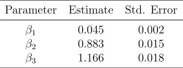
The parameter vector to estimate is (θ, β). The vector θ projects the actual revenue from exporting, Rict, onto the vector of firm and country characteristics XictR. The vectorβ transforms revenue from exporting into variable profits (β1) and parameterizes the fixed costs from exporting (β2 and β3).
We follow a two-step estimation procedure. In the first stage, we apply panel data estimation techniques to obtain point estimates ofθ that are independent of the value estimated forβ. In the second stage, we use the moment inequality framework described in Section 3 in order to obtain set estimates forβ that are conditional on the first stage estimates of θ.39
Using data on observed export revenues for firms, countries and years with positive exports, we obtain an estimate for θ. Section 2 of the Online Appendix describes the estimation ofθ in detail. The outcome of this first stage is the variable ˆRict =r(XictR; ˆθ) and we use it to proxy forRict∗ :
Uict =β1Rˆict−β2−β3Dc+νict+εict, (37)
where νict =νictπ +β1E
Rict−Rˆict|Jict], and εict =β1(Rict∗ −Rict) +β1
(Rict −Rˆict)−
E
Rict −Rˆict|Jict]
. The structural error, νict, incorporates both the determinants of the static profits the econometrician does not observe, νictπ , as well as the part of the approximation error from the first stage,Rict - ˆRict, that is in the information set of the exporter. The measurement error,εict, incorporates both the expectational error, R∗ict -Rict, and approximation error from the first stage that is orthogonal to the information set of the exporter.
We impose Assumptions 1 and 3 to the distribution of (νict, εict) conditional on (Xict∗ , Zict) and assume that νict is iid across firms, countries and time periods and normally distributed with mean 0 and variance equal to 1.40 Assumption 1 imposes exogeneity restrictions that are common in the international trade literature: unobserv-able (to the econometrician) determininants of entry in a give