Accounting for Tuition Increases across U.S. Colleges
∗Grey Gordon
Federal Reserve Bank of Richmond†
Aaron Hedlund University of Missouri‡ December 27, 2018
Abstract
This paper uses detailed institution-level data and an equilibrium model to assess differ-ent theories for the steep, persistdiffer-ent rise in college tuition. The framework embeds quality-maximizing, imperfectly competitive colleges into an incomplete markets, life-cycle environment with student loan borrowing and default. We measure the contribution of supply-side factors— namely, Baumol’s cost disease and changes in the availability of non-tuition revenue sources—as well as demand-side forces, such as evolutions in the college earnings premium and changes to the Federal Student Loan Program. Together, these forces explain the entire increase in net tuition since 1987 with increases in demand playing the largest role.
Keywords:Higher Education, College Costs, Tuition, Student Loans, Baumol Cost Disease JEL Classification Numbers:E21, G11, D40, D58
∗
We thank our discussant Alex Monge-Naranjo as well as Kartik Athreya, Sandy Baum, Bruce Chapman, Sue Dynarski, Gerhard Glomm, Bulent Guler, Kyle Herkenhoff, Jonathan Hershaff, Brent Hickman, Felicia Ionescu, John Jones, Michael Kaganovich, Oksana Leukhina, Lance Lochner, Amanda Michaud, Chris Otrok, Urvi Neelakantan, Irina Shaorshadze, Yu Wang, Fang Yang, Constantine Yannelis, Eric Young, and seminar participants at the Econo-metric Society NASM 2017, SED 2017, the CEPR Workshop on Financing Human Capital, and the Philadelphia Fed Conference on Consumer Finance and Macroeconomics. This material is based upon work supported by the National Science Foundation under Grant Numbers 1730078 and 1730121. Any opinions, findings, and conclusions or recommendations expressed in this material are those of the authors and do not necessarily reflect the views of the National Science Foundation, the Federal Reserve Bank of Richmond, or the Federal Reserve Board of Governors.
†
E-mail:[email protected]
1
Introduction
Over the past few decades, the stubborn upward march of college tuition across all major
seg-ments of higher education has led to growing concerns about access, affordability, and mounting student loan debt. Among selective, frequently wealthy private research institutions, net tuition—
that is, sticker price minus institutional aid coming in the form of need-based and merit-based
scholarships—increased by 50% between 1987 and 2010 in real terms (from $15,500 to $23,700 in constant 2010 dollars) and by an astonishing 140% (from $2,700 to $6,400) for non-selective public
teaching colleges that tend to be more resource constrained.1 Several explanations have emerged
to explain these and other higher education trends pertaining to enrollment, graduation, and post-graduation outcomes, but little consensus has emerged regarding their quantitative salience. While
some explanations highlight the importance of broad macroeconomic forces, such as rising labor market skill premia that increase the value of a college degree, others focus on college-specific factors
such as cuts in state support or the unintended consequences of federal student aid.
This paper quantitatively evaluates several prominent theories of tuition inflation using detailed micro-data and a rich equilibrium macroeconomic model that incorporates several key features of
the higher education landscape. To organize thinking, we separate the theories which involve factors
that directly affect college supply from those that revolve around forces that shift demand. On the supply side, Baumol’s cost disease emphasizes the commonality between higher education and other
service sectors, where the stipulated combination of stagnant productivity growth and rising labor
costs creates persistent inflationary pressures. Another common supply-side explanation focuses on the role of declining state support for public institutions. We analyze this theory both independently
and within the broader context of changes to other sources of non-tuition revenue. On the demand
side, we examine the frequently-mentioned Bennett hypothesis, which attributes higher tuition to the same federal student aid programs that are meant to help with college affordability. Specifically,
we assess the contribution of pre-Great Recession reforms to the Federal Student Loan Program
(such as the addition of unsubsidized loans in 1993) in addition to the evolution of loan limits, interest rates, and Pell Grants. Lastly, we also quantify the role of rising labor market skill premia
and higher parental income through their impact on college demand.
With the presence of extensive public subsidies, complicated financial aid rules, market power, and widespread price discrimination, higher education functions quite differently from most other
markets. Furthermore, non-profit institutions—which are the focus of this paper—face different
objectives and incentives than profit-maximizing firms. To capture these features, we assume that colleges maximize quality, which is a function of per-student investment and average student ability,
just as in the static models of Epple, Romano, and Sieg (2006) and Epple, Romano, Sarpca, and Sieg (2013). By operating with market power, colleges engage in price discrimination to balance
student recruitment against the need to raise revenue for quality-enhancing investment. Students,
1
in turn, weigh cost and quality when choosing from among the set of colleges to which they receive
an offer of admission. In equilibrium, the endogenous sorting of students across colleges affects both dimensions of the college quality distribution, which creates a computationally challenging fixed
point problem. Our quantitative framework does well at capturing this sorting.
We find that the aforementioned theories in conjunction can explain the entire 107% increase in average college net tuition since 1987. However, across institutions, the contribution of any one
factor varies based on the differing circumstances faced by each college type. Overall, our estimates
indicate that demand-side changes have driven most of the rise in tuition, with student loan policy changes alone accounting for a 42% increase. On the supply side, we find only modest support for
Baumol’s cost disease. Lastly, changes intotal non-tuition revenue have actually held down tuition
by 7% for public institutions and 23% for private institutions.
1.1 Related Literature
A growing literature employs general equilibrium models to analyze higher education while taking
the behavior of colleges and tuition as given. For example,Abbott, Gallipoli, Meghir, and Violante
(2016) develop an equilibrium model to analyze financial aid policies intended to promote college
at-tendance. Their framework features a rich intergenerational setting, intervivos transfers, and college
attendance financed partly by grants and loans. In other work, Athreya and Eberly (2016) study the impact of a rising college wage premium on college attainment in the presence of heterogeneous
drop-out risk and post-graduation earnings risk. Hendricks and Leukhina (2016) and Chatterjee
and Ionescu(2012) also investigate the importance of drop-out risk for college attainment.Garriga and Keightley(2010), Lochner and Monge-Naranjo(2011),Belley and Lochner(2007), andKeane
and Wolpin(2001) also develop equilibrium models to answer various important questions that lie
at the intersection of macroeconomics and higher education.
This paper endogenizes tuition and the response of colleges to evolving market conditions and
policies. In this vein, recent work by Jones and Yang (2016) closely mirrors the objectives here.
They explore the role of skill-biased technical change in explaining the rise in college costs from 1961 to 2009. However, their study differs from this paper in several ways. First, this paper takes
a unified look at both supply-side and demand-side factors that influence tuition, whereas they
focus on the role of cost disease. Second, the object of interest inJones and Yang (2016) is college costs, which increased by 35% in real terms between 1987 and 2010, whereas this paper addresses
the much larger 92% increase in net tuition. Also, whereas they use a competitive, representative
college framework, this paper employs a model with heterogeneous, imperfectly competitive colleges, peer effects, and student loan borrowing with default. Fillmore(2016) and Fu (2014) develop rich
frameworks with heterogeneous colleges, but in both cases, students have static, reduced-form utility functions. Furthermore, peer effects are exogenous inFillmore(2016), andFu(2014) does not allow
Methodologically, the most closely related papers are Epple et al. (2006), Epple et al. (2013),
and our earlier paper,Gordon and Hedlund(2016). The former two papers develop a static model of heterogeneous, quality-maximizing colleges that operate in an environment of imperfect competition
and engage in price discrimination.Gordon and Hedlund(2016) embed this framework in a broader
macroeconomic model but consider only the case of a single, monopolistic college. Such a case greatly simplifies computation but implies exaggerated market power with colleges facing no competitive
pressure besides that provided by the outside option of skipping college entirely. This paper takes
the important step of adding heterogeneous colleges, which allows for rich competition and sorting. This paper also relates to a large empirical literature that estimates the effects of macroeconomic
factors and policy interventions on tuition and enrollment. The origins of cost disease emerge from
seminal works by Baumol and Bowen(1966) andBaumol(1967). They lay out a clear mechanism: productivity increases in the economy at large drive up wages everywhere, which service sectors
that lack productivity growth pass along by increasing their relative prices. Recently, Archibald
and Feldman (2008) use cross-sectional industry data to forcefully advance the idea that cost and price increases in higher education closely mirror trends for other service industries that utilize
highly educated labor. In short, they “reject the hypothesis that higher education costs follow an
idiosyncratic path.”
The empirical literature has conflicting findings on the impact of state higher education
ap-propriation on college tuition. For example,Heller(1999) suggests a negative relationship between state support and tuition, asserting that “the higher the support provided by the state, the lower
generally is the tuition paid by all students.” Recent empirical work by Chakrabarty, Mabutas,
and Zafar (2012), Koshal and Koshal (2000), and Titus, Simone, and Gupta (2010) support this hypothesis, but notably, Titus et al.(2010) show that this relationship only holds up in the short
run. Lastly, in a large study commissioned by Congress in the 1998 re-authorization of the Higher
Education Act of 1965,Cunningham, Wellman, Clinedinst, Merisotis, and Carroll(2001a) conclude that “decreasing revenue from government appropriations was the most important factor associated
with tuition increases at public 4-year institutions.”
Shifting to demand-side factors, the empirical literature is split on the impact of financial aid on tuition. For example, McPherson and Shapiro (1991), Singell and Stone (2007), Rizzo and
Ehrenberg (2004), Turner (2012), Turner (2013), Long (2004a), and Long (2004b) find at least
some evidence in support of the Bennett hypothesis, though they disagree on the magnitude of the pass-through of aid into higher tuition and whether public or private institutions are more
responsive. Most recently, Lucca, Nadauld, and Shen (2015) find a 65% pass-through effect for
changes in federal subsidized loans and positive but smaller pass-through effects for changes in Pell Grants and unsubsidized loans. Similarly, Cellini and Goldin (2014) show that tuition is 78%
higher at for-profit colleges that participate in federal student aid compared to those that do not.
Act,Cunningham et al.(2001a);Cunningham, Wellman, Clinedinst, Merisotis, and Carroll(2001b)
conclude that “the models found no associations between most of the aid variables and changes in tuition in either the public or private not-for-profit sectors.”Long (2006) and Frederick, Schmidt,
and Davis(2012) echo these sentiments.
We also analyze how labor market trends over the past few decades have impacted tuition. Empirically,Autor, Katz, and Kearney (2008) report that the college earnings premium increased
from 58% in the mid-1980s to 93% in 2005, which Autor et al. (2008), Katz and Murphy (1992),
Goldin and Katz(2007), andCard and Lemieux (2001) ascribe to skill-biased technological change and a fall in the relative supply of college graduates. In recent work, Andrews, Li, and Lovenheim
(2012) and Hoekstra (2009) study the distribution of college earnings premia and find substantial
heterogeneity attributable to variation in college quality.
2
The Model
The model consists of heterogeneous, finitely-lived households, heterogeneous colleges, and the government.
2.1 Colleges
There is a finite number K of college types with each k∈K representing a positive measure g(k) of identical colleges. Each college maximizes quality, which depends positively on average academic ability of the student body, investment per student, and total enrollment while depending negatively
on average parental income, as inEpple et al.(2006). School types differ exogenously along several
dimensions, and additional heterogeneity arises in equilibrium from endogenous sorting.
The first source of heterogeneity enters the college budget constraint, with colleges of type
k receiving non-tuition public (private) support Eg,k(Nk) (Ep,k(Nk)) and facing operating costs
Ck(Nk), where Nk is enrollment. Next, colleges differ in terms of their student retention
proba-bilities and post-graduation labor market outcomes. Specifically, students attending college typek
face an annual dropout risk ofδk(sY) and earnings premia ofλk(sY), both of which also depend on
the student’s type sY. We take the student’s type as consisting of an “ability” measure x (which
includes any innate ability and embodied human capital as of age 18) and parental income y. To keep the model tractable, we follow Gordon and Hedlund(2016) by introducing additional assumptions that make the college problem each period independent of past decisions. Doing so
allows us to analyze rich peer effects, sorting, and imperfect competition in equilibrium without the
additional complications of strategic investment and dynamic market power. To be concrete, we first assume that colleges are subject to an annual balanced budget constraint. Instead of actively
managing an investment portfolio, colleges simply receive an exogenous flow of non-tuition revenue
from endogenous tuition. Secondly, we assume that, after making admissions, tuition, and spending
decisions for each incoming cohort, colleges immediately sell the associated stream of future cash flows to a deep pocketed intermediary in exchange for the expected, undiscounted sum of these
cash flows.2 In terms of practical effect, the college commits to keeping tuition and spending fixed
for each cohort, and there is no cross-cohort subsidization. The expected stream of payments for an incoming student with annual dropout probabilityδ paying net tuition T (defined as sticker price
T minus institutional aid) isT, (1−δ)T, . . . ,(1−δ)JY−1T. Definingω =PJYj=1(1−δ)j−1, the net present value of these payments is T ω.
What is the objective function of a non-profit college? Following Epple et al. (2006,2013), we
assume they maximize quality, a function of average abilityX and quality-enhancing spending per student I. While the results of Epple et al. (2006, 2013) and our benchmark results show this assumption will give nice quantitative predictions, the appendix provides several additional pieces
of evidence in favor of this assumption. Additionally, for better quantitative properties, we allow
quality also to depend on the student body size N—which will let us better match the large and comparatively cheap tuition at public schools—and, inversely, on average parental income Y— which, through correlations between income and race, allows for a diversity or affirmative action
motive.
We introduce tuition discounting and matching of students with colleges via competitive search.
In this setup, students and admissions vacancies at each college type are matched frictionally in submarketsm≡(k, T, sY) indexed by the college typek, net tuitionTand student typesY = (x, y).
We use the notation k(m), T(m), x(m), y(m) to select the various components of m. Vacancies cost κ and are filled with probability ρ(θ(m)), with students and colleges taking the tightness
θ(m)—that is, the ratio of vacancies to search-intensity-adjusted applications—as given. A college of type k’s problem is
max
v(m)≥0q(X, Y, I, N)
s.t.pIN+pC(N) +κ
Z
v(m)dm=
Z
T(m)ω(m)v(m)ρ(θ(m))dm+Eg(N) +Ep(N)
X =
Z
x(m)ω(m)v(m)ρ(θ(m))dm/N
Y =
Z
y(m)ω(m)v(m)ρ(θ(m))dm/N
N =
Z
ω(m)v(m)ρ(θ(m))dm
(1)
with vacancies only in the college’s own type ((k(m)−k)v(m) = 0). The interior solution states
2
that, in active submarkets, tuition satisfies
T(m) = κ
ω(m)ρ(θ(m))
| {z }
Search premium
+
EM C(sY)
z }| {
pI+pC0(N)−Eg0(N)−Ep0(N)
| {z }
Marginal resource cost
− pqN qI
N
| {z } Size discount
−pqX qI
(x−X)
| {z }
Ability discount
− pqY qI
(y−Y).
| {z }
Low income discount
(2)
If, for a givenθ(m)>0, a submarket hasT(m) strictly greater than the right hand side, the college would post an infinite number of vacancies implying θ(m) should be infinite, which cannot happen in equilibrium. Conversely, if for a given θ(m) > 0 a submarket has T(m) strictly less than the right hand side, the college would post no vacancies, implying θ(m) should be zero and hence not an active submarket.
Absent search frictions (κ = 0), students pay individual-specific net tuition equal to their effective marginal cost EM C(sy), which is a term first coined by Epple et al. (2006). Intuitively,
each student tightens the college’s budget constraint bypI+pC0(N)−Eg0(N)−Ep0(N), but they also contribute to college quality based on their characteristicssY, as shown by the last three terms
of (2). The role of search (κ >0) is then to introduce a markup representing college market power.
2.2 Households
Households go through three phases of life: youth, working age, and retirement.
2.2.1 Youth
Each period, a fixed measure of heterogeneous youths with characteristics sY = (x, y) enter the
economy at age j = 1 corresponding to high school graduation. Their main decision is whether to immediately join the workforce (k = 0) or attend a college k ∈ {1, . . . , K}. While enrolled, students receive additive utility v(qk) that depends positively on college quality qk. In addition, higher educational attainment (and especially graduation) delivers future labor market benefits. Youth who skip college and directly enter the labor market receive earnings µjez where µj is an
age-specific deterministic profile and z follows a random walk with z0 = 0 and innovations σε.3
For youth who attend college, graduation confers a log earnings premiumλk(sY) that is specific to
college kand individuals with characteristics sY. To graduate, a student must not dropout for JY
periods where the annual dropout probability is δk(sY). Students who dropout after attending for
j years receive a prorated premium ofλk(sY)j/(JY + 1), which will imply a 17% sheepskin effect
in our calibration.
When making the decision to attend college k, a youth of type sY must also choose a desired
net tuition level T, implicitly choosing a submarket m = (k, T, sY). Naturally, students prefer to
pay lower tuition, but acceptance probabilitiesη(θ(m)) increase inT. (For instance, in equilibrium
the probability of being accepted in a submarket withT < EM Ck(sY) must be zero.) Rather than
explicitly model the choice of students to apply to several colleges within typek, we assume that, conditional on choosing submarket m, students exert search intensity s ≥ 1 to ensure they get admitted to a college within that type, i.e.sη(θ(m)) = 1.4 Thus, students trade off the cost of net tuition T against the search disutilityψ(s−1)2.
Besides net tuition T, students face non-tuition expenses φ. These total costs T +φ can be covered using a combination of personal and family resources, student loans, and government
grants. Eligibility for need-based grants ζ(T +φ, EF C(sY)) depends on EF C(sY), which is the
expected family contribution formula. After subtracting these grants, the net cost of attendance
N COA(T, sY) =T +φ−ζ(T +φ, EF C(sY)) acts as a ceiling on the amount students can borrow
through the Federal Student Loan Program (FSLP).
The FSLP contains two main borrowing instruments. Subsidized loans are the most financially
attractive because they do not accrue interest while the student is enrolled in college. For this
program, eligibility depends on financial need, defined asN COA(T, sY)−EF C(sY). Also, beginning
in 1993, the government has allowed students to borrow the remainder of their education costs up
toN COAusing unsubsidized loans that do accrue interest during college.
In addition to the constraint that borrowing cannot exceed N COA, students face annual and aggregate limits for subsidized and combined borrowing (i.e., subsidized plus unsubsidized). Let ¯bj
denote the annual combined borrowing limit for a agej youth and ¯l the aggregate combined limit. Then subsidized borrowingbs and unsubsidized borrowingbu must satisfy
bs+bu≤min{¯bj, N COA(T, sY)}. (3)
Additionally, the choice of subsidized and unsubsidized loans, denoted as l0s and l0u, respectively, must be less than ¯l. Analogously, define bsj as the statutory annual subsidized limit and lsj as the statutory aggregate subsidized limit. Annual subsidized borrowing bs must be less than ¯bsj, and
total subsidized borrowing l0s must be less than ¯lsj.
Apart from loans, students have two other means of paying for college. First, they have earnings
eY, which we treat as an endowment. Second, they receive a parental transferξEF C(sY), where
ξ∈[0,1] is a parameter. The budget constraint for a type-sY college student is
c+N COA(T, sY)≤eY +ξEF C(sY) +bs+bu. (4)
Our calibration ofξwill capture data on parental transfers, irrespective of whether they are financed by PLUS Loans, second mortgages, or credit card borrowing.
4
2.2.2 Workers and Retirees
Workers and retirees receive non-asset income based on their level of education, age, retirement
status, and a stochastic component that follows a random walk with innovations ε ∼ N(0, σz2). This income is then taxed at a proportional rate τ. Consumption provides period utility u(c), and the future is discounted at rate β. Workers with student loans owe constant payments of
p(l, t) = li(1+(1+ii))tt−−11 that amortize the remaining balance l at interest ratei over the t years left on
the loan. Under current law, default has two costs. First, collection charges of up to 25% of the outstanding principal may be added to payments. We model this via a penaltyη added to the loan when the household first defaults. Second, wages and tax refunds may be garnished. We model this
as a wage garnishment γ that remains until the household rehabilitates the loan (by resuming on time payments) or pays it off. Households in the model cannot engage in borrowing outside of the
student loan program, but they can save using discount bonds having a price 1/(1 +r).
2.3 Value Functions
Workers with loans in good standing choose whether to default or make a payment,
Vj(a, l, t, z, f = 0) = max{VjR+1(a, l, t, z), VjD+1(a, l(1 +η), z)}. (5)
whereVR is the value of repayment andVD is the value of default. The decision to default results in a proportional balance penalty η added to the loan.
Workers in a state of delinquency choose whether or not to rehabilitate their student loan,
Vj(a, l, z, f = 1) = max{VjR+1(a, l, tmax, z), VjD+1(a, l, z)} (6)
where rehabilitation resets the loan repayment clock totmax.
The value function for workers who make a loan payment is
VjR(a, l, t, z) = max
a0≥0u(c) +βEε0Vj+1(a 0
, l0, t0, z+ε0,0) s.t. c+a0/(1 +r) +p(l, t)≤(1−τ)µjez+a
l0= (l−p(l, t))(1 +i)
t0 = max{t−1,0}
(7)
The value of choosing to remain in default is
VjD(a, l, z) = max
a0≥0u(c) +βEε0Vj+1(a 0
, l0, z+ε0,1) s.t.c+a0/(1 +r)≤(1−γ)(1−τ)µjez+a
l0 = max{0,(l−γ(1−τ)µ ez)(1 +i)}
whereγ is the lost fraction of earnings from wage garnishment.
Upon matriculation, each college student has an associated drop-out probability δ, net tuition
T, expected family contributionEF C, and log-college earnings premium λas state variables with a value function
e
Yj(l;λ, δ, T, EF C) = max
c≥0,l0≥lu(c) +β h
(1−δ)1[j<JY]Yej+1 l0;λ, δ, T, EF C
+ (1−δ)1[j=JY]Eε0Vj+1
0, l0, tmax, λ+σz(j+ 1)1/2ε0,0
+δEε0Vj+1
0, l0, tmax, λ
j JY + 1
+σz(j+ 1)1/2ε0,0
s.t.c+T ≤eY +ξEF C+bs+bu+ζ(T+φ, EF C)
N COA=T +φ−ζ(T +φ, EF C)
bs=l0s−ls, bu=
l0u
1 +i−lu
bu ≤min{¯buj, N COA}, bs+bu ≤min{¯bj, N COA}
ls0 + l
0 u
1 +i ≤
¯
l
(9)
where the decomposition of total loan balances into subsidized/unsubsidized components is
(ls0, lu0) =
(
(l0,0) ifl0≤elsj(N COA, EF C)
(eljs(N COA, EF C), l0−elsj(N COA, EF C)) otherwise
(ls, lu) = (
(l,0) ifl≤elsj−1(N COA, EF C)
(elj−s 1(N COA, EF C), l−elj−s 1(N COA, EF C)) otherwise.
(10)
Note that the college earnings premium gradually increases with each year of enrollment, and there
is a discrete jump upon graduation to reflect the sheep-skin effect.
The value of attending college k (before preference shocks) is given by
Yk(T, sY) =Ye1(0;λk(sY), δk(sY), T, EF C(sY)) + JY X
j=1
βj−1(1−δk(sY))j−1v(qk). (11)
The value of not attending college is defined as
ˆ
Y0(sY) =Eε0V1(0,0,0, ε0,0), (12)
Conditional on applying to college k, the youth’s choice of T and search intensityssolves
ˆ
Yk(sY)≡ max
s≥1,Tmin{sη(θ(m)),1}(Y k(T, s
Y)−Yˆ0(sY)) + ˆY0(sY)−ψ(s−1)2
s.t. sη(θ(m)) = 1
m= (k, T, sY)
(13)
wherek= 0 is the decision to skip college andMk(sY) ={(Tk, sY)}. Simplifying, this is
ˆ
Yk(sY) = max T Y
k(T, s
Y)−ψ(1/η(θ(m))−1)2
s.t. m= (k, T, sY)
(14)
Lastly, to account for unobserved preferences, we add idiosyncratic taste shocks when the
stu-dent is choosing k:
max
k∈{0,...,K}
ˆ
Yk(sY) +
1
σε
k. (15)
These preference shocks introduce non-pecuniary benefits of attending specific colleges, which
re-sults in smoother, more mixed sorting behavior of student types across colleges.
Assuming the taste shocks are distributed according to a Type 1 extreme value distribution,
the probability of choosing college kis
Ak(sY) :=
exp(σ( ˆYk(sY)−Yˆ0(sY)))) PK
˜
k=0exp(σ( ˆY ˜ k(s
Y)−Yˆ0(sY)))
. (16)
Because we assume that applicants must jointly choose submarkets and search effort to guarantee
attendance, this probability is also the attendance rate for typesY.
2.4 Government
The government levies proportional taxes on labor earnings to fund transfers and loans (both
subsidized and unsubsidized) to students in college. Other sources of revenue for the government
include interest payments on unsubsidized loans for students in college as well as loan payments and garnishment from workers with outstanding student loans.
2.5 Equilibrium
A steady state equilibrium consists of market tightnesses θ, college vacancy postings vk, value functions Yk, ˆYk, and V, application rates Ak, and tax rates such that
1. colleges optimally choosevk taking market tightnesses as given;
3. application ratesAkand market tightnessesθkare consistent with the student value functions
Yk,Yˆk and vacancy creationvk; and
4. the government balances its budget.
While we compute steady state equilibria to ensure the FSLP budget balances given its
pay-as-you-go structure, all the other equilibrium conditions are for a given cohort. Consequently, a better way to think of the equilibrium may be as a cohort-specific equilibrium where the government can
fund the FSLP at zero interest.
3
Data, Calibration, and Estimation
We now turn to the calibration and estimation of the model.
3.1 College Data and Types
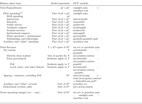
Colleges are large, multifaceted organizations, and this complexity manifests itself in their balance sheets. In line with the model, we distill college budgets into net tuition revenue T, non-tuition revenue E, operating costs pC, recruiting costs K ≡ κR vdm, and quality-enhancing investment
pI. The budget constraint we work with for accounting purposes is
pI +pC+K =T+Eg+Ep. (17)
Table 1 provides the mapping between model and data using institution-level IPEDS data from the Delta Cost Project (DCP). As the distinction between quality enhancing expenditures and
other expenditures is not obvious in the data, we do not try to separately identify the expenditure
components in the data.
We break schools into seven types based on three criteria: Whether they are public (G) or
private (P), teaching (T) or research-intensive (R) as defined by the Carnegie Classification; and
selective (S) or non-selective (N). The selectivity metric is based on whether the mean SAT score is above 1250 (in a 1600 point system) or not. For some schools, we must impute this measure, and the
details are in the appendix. At times, we will use the abbreviations to designate school types with,
e.g., PRS denoting private, research-intensive, selective schools. There are not eight types because GTS schools do not exist according to our classification. Summary statistics by school type and
year—including the budgetary items discussed above—are given in table 9 in the appendix, but
Balance Sheet Item Model Equivalent
Total Expenditures pI +pC+K
E&G Spending Component ofpI +pC+K
Auxiliary and “Other” Spending Component ofpI +pC+K
Total Revenue T+Eg+ Component ofEp
Net Tuition T
Directly from Student Out of Pocket forT
From Government Students Pay TowardsT
Pell Students Pay TowardsT
Local, State, and Other Federal Students Pay TowardsT
Approp., Contracts, Excluding Pell Eg
Auxiliary and “Other” Revenue Subcomponent ofEp
Endowment Revenue, Gifts Subcomponent ofEp
Gross Operating Margin (Rev. −Exp.) Remainder of Ep
Notes: Ep = “Component of Ep” + “Remainder of Ep.” We only
distinguish betweenpI, pC and K in the model as the empirical dis-tinction is not clearcut.
3.2 Mapping of Model to Data Units
One unit of the consumption good is treated as $1,000 in 2010 dollars. We take ability to be
uniformly distributed between 0 and 1 and measure it using the AFQT for students.5 We assume
that enrollmentN corresponds to a school’s full-time equivalent (FTE) share in the data multiplied by the enrollment rate. The number of schools within each type g(k) is given by the number of schools in the data. (There is virtually no school entry or exit in the data over this time period,
so we assume it is time-invariant.) The number of schools plays a material role in limiting market power at school types having large g(k)—all coming through changes in market tightness which measure aggregate postings of a school type. In particular, PTN, GTN, and PRN have between
120 and 640 schools while the selective schools range from 20 to 42. Table 2 summarizes how we map the data and model populations.
Data Model
Youth population 1
Number of schools within each type g(k) A school’s FTE share ×the enrollment rate N
Table 2: Mapping between the data and model
3.3 College Quality
We assume q is given by a CES quality function
q(X, Y, I, N) =
αXX −1
+αYY− −1
+αII −1
+αNN −1
−1
. (18)
Note thatY is a “bad” because its exponent is−(−1)/ <0.
Note that, while the model has extremely tight predictions about net tuition for each student, it is silent regarding the pre-institutional aid “sticker price” tuition. To overcome this shortcoming
and allow sticker prices in the data to help discipline the quality function parameters, we construct
an artificial sticker price in the model. To do so, we use the percentage of students receiving institutional grants in the data to construct a cutoffT such thatP(T ≤ T) is the fraction receiving institutional grants. We then take E(T|T >T) as the “sticker price.”
With the sticker price defined asE(T|T >T), we can then use the disparity in sticker price and
net tuition to disciplineαX/αI and(which play a crucial role in determining the ability discounts).
Likewise,αY/αIandare disciplined by the average parental income across schools. LargerαN/αI
depresses tuition uniformly and expands enrollments, and so the level of net tuition and enrollments
5For colleges, we will sometimes refer to a relative ability measure. This measure assumes SAT scores of college
helps identify them, and we allow αN to differ by whether the school is public or private. Jointly
αX, αY, αN, αIcannot be separately identified because scaling them all by a constant represents the
same preferences. Hence, we normalizeαX to be 1. Consequently, the quality function has five free
parameters, which we will identify using 42 cross-sectional moments (an observation for each of the
school types for net tuition, sticker price tuition, expenditures, enrollments, ability, and parental income).
3.4 Non-Tuition Revenue and Operating Costs
We use linear specifications Eg(N) = Eg,kN and Ep(N) = Ep,kN for non-tuition revenue and, followingEpple et al.(2006), we posit operating costs of the form
C(N) =ck0 +c1kN+ck2N2. (19)
Rather than calibrate 3Kparameters, we simplify the process by using information from a “nearby” problem. Specifically, we first assume that ck1 = 0 for all k. Next, we consider the solution to the college problem under the assumption that there is no student heterogeneity. Under these
assumptions, one can show the optimal choice of colleges must satisfy
qN
qI
+1
p
d(E(N)/N)
dN =
d(C(N)/N)
dN (20)
whereqN/qI is (αN/αI)(N/I)−1/.
For calibrating theck0, ck1, ck2 parameters, we assume that enrollments in the data correspond to the efficient scale given by the solution to this problem, i.e. Nk = N. Given I and Nk, the cost parameters ck2 and ck0 are related by
ck2(Nk)2=ck0+αN
αI
Nk I
!−1/
(Nk)2. (21)
We do not take a stand on which components of college spending per FTE Sk in the data are operating costs and which represent quality-enhancing investment. Instead, we simply proxy for I
by assuming it is two-thirds of average expenditures per FTE in the data, i.e., Ik = 231pSk. After this process, onlyK cost parameters remain: ck0 for each k.
To discipline each fixed costck0, we assume it is a proportion c∈[0,1] of total expenditures,
ck0 =c1
pS
k
Nk. (22)
3.5 Matching Technology
We assume a CES matching function for vacancies v and intensity-adjusted applicantsue=suis
m(eu, v) =uemin
A(v/ue)
(1 + (v/eu)
γ)1/γ,1
(23)
The resulting matching rate for intensity-adjusted applicants isη(θ) = m(eu,v) e
u = min
n Aθ (1+θγ)1/γ,1
o
,
where θ = v/ue is the market tightness. Analogously, the matching rate for vacancies is ρ(θ) =
η(θ)/θ. We set γ = 1 and then choose A such that students and colleges match with a 95% probability whenθ= 1, which givesA= 2·0.95.
3.6 Dropout Risk and Earnings Premia
Graduation rates and labor market premia depend both on school type and individual student
ability. To best match the data while maintaining tractability of estimation, we assume a constant
weight µδ for the contribution of college type. Specifically,
(1−δk(x)) = minnmaxn1−δk µδ+ (1−µδ)
x Xk
,0o,1o (24)
whereδk is from the data (specifically, the institution level data),x is individual ability, andXk is average ability at school k.
To determine µδ, we first compute average ability and graduation rates by college type, as
defined by sticker tuition quintile. Next, we regress graduation on a quintile dummy multiplied by
the average graduation rate times the ratio of individual ability to average ability. The results are presented in Table 19 in the appendix. Except for the lowest quintile, the relationship between
ability and graduation is statistically significant and stable at around 40%. Consequently, we take
µδ= 0.6.
We follow a similar procedure for the college earnings premium by assuming that
λk(x) =λk
µλ+ (1−µλ)
x Xk
(25)
and replacing the graduation dummy on the left side of the regressions with the log college premium. The results, which also appear in Table19, are relatively stable across the quintiles and lead us to
setµλ = 0.1. Note that ak-invariantµλ in no way implies similar college premia across colleges. In
fact, using the NLSY97 data, we find the log college premium for the lowest quintile is 0.363 while
3.7 Parental Transfers
We use NLSY97 data to calibrate the fraction ξ of parental transfers that appear directly in the student budget constraint, i.e. ξEF C(sY). The first step involves computing parental income and
applying the simplified formula fromEpple et al.(2013) to get an EFC measure (the same as in the model). Next, we use data on family aid for college that is not expected to be paid back and find
the annual level of support. Lastly, we regress this transfer measure on interaction terms between
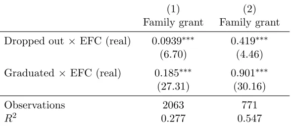
EFC and whether a student dropped out or graduated. We do this for two samples, the full sample and a subsample whereEF C is less than net tuition, expecting transfers are not unconditional but contingent on having sufficiently large college costs. The results, which are given in Table 3, lead
us to set ξ= 0.7, loosely the midpoint of 0.419 and 0.901.
(1) (2)
Family grant Family grant
Dropped out×EFC (real) 0.0939∗∗∗ 0.419∗∗∗
(6.70) (4.46)
Graduated×EFC (real) 0.185∗∗∗ 0.901∗∗∗
(27.31) (30.16)
Observations 2063 771
R2 0.277 0.547
tstatistics in parentheses
(1) is the full sample; (2) includes only those with EFC<net tuition. ∗
p < .1,∗∗ p < .05,∗∗∗p < .01
Table 3: Transfers as a function of EFC
3.8 Household Preferences
In the benchmark, we assume v(·) = 0 so that college quality does not change utility. The flow utility is standard with a constant relative risk aversion of two. We take the time discount factorβ
to be 0.96. Search intensity disutility ψis jointly estimated, as is the preference shock size σ.
3.9 Jointly Estimated Parameters
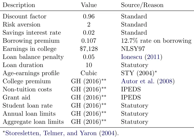
Table4 summarizes the calibration of most non-college-specific parameters. The remaining param-eters are jointly estimated to fit a large number of moments ranging from net and sticker tuition,
enrollment shares, expenditures, enrollment rates, and ability at each school type along with the
correlation between parental income and enrollment. Table 5 provides a summary. Of note, the calibrated value for c turns out to be quite small, implying fixed costs are relatively unimportant
Description Value Source/Reason
Discount factor 0.96 Standard
Risk aversion 2 Standard
Savings interest rate 0.02 Standard
Borrowing premium 0.107 12.7% rate on borrowing
Earnings in college $7,128 NLSY97
Loan balance penalty 0.05 Ionescu (2011)
Loan duration 10 Statutory
Age-earnings profile Cubic STY (2004)∗ College premium GH (2016)∗∗ Autor et al. (2008) Non-tuition costs GH (2016)∗∗ IPEDS
Grant aid GH (2016)∗∗ IPEDS
Student loan rate GH (2016)∗∗ Statutory Annual loan limits GH (2016)∗∗ Statutory Aggregate loan limits GH (2016)∗∗ Statutory
∗Storesletten, Telmer, and Yaron(2004).
∗∗Web appendix A ofGordon and Hedlund(2016).
Table 4: Independently determined model
Description Parameter Value
Preference shock size σ 8.062
Vacancy posting cost κ 0.008
Search effort level ψ 1000.000
Cost parameter c 0.001
Quality’s elasticity 0.525
Quality’s weight on investment αI 31.805
Quality’s weight on enrollmentN, public schools αgN 0.133 Quality’s weight on enrollmentN, private schools αpN 0.088 Quality’s weight on inverse parental incomeY−1 αY 0.012
private schools, consistent with the quadratic term capturing capacity constraints that are tighter
at small schools. The search intensity parameterψ is very large, which implies students only go to submarkets where they get in with zero search intensity.6 The vacancy posting costκends up small
(as a share of total revenue, total posting costs are on the order of 0.01%) implying there is not
much market power. The preference shockσ ends up being large with a standard deviation shock being worth around 12% of lifetime consumption.7 The quality elasticity parameterimplies more complementarity than Cobb-Douglas.
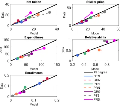
Because of the large number of targeted moments, it is most convenient to represent the model fit graphically, as shown in figure1. Each blue dot represents a college type, with the vertical position
giving the data moment and the horizontal position showing the model moment. A perfect fit would
be represented by all the blue dots falling along the 45-degree line. Figure 1 also labels the worst fitting school type. For instance, the worst fit for net tuition comes from GRS (where, as discussed
earlier, G stands for public, R stands for research, and S stands for selective). Similarly, the worst
fit for FTE share comes from PTN (which stands for private (P), teaching (T), nonselective (N) schools). Overall, the model does a good job of matching the targeted moments, except for parental
income which received a lower weight in the GMM estimation.
4
Results
This section assesses whether the theories from section 1 can jointly explain the large rise in net
tuition between 1987 and 2010 while also demonstrating consistency with other empirical trends.8 Following this joint analysis, we undertake a quantitative decomposition to measure the
conse-quences of each theory individually both for aggregates and across institution types.
4.1 Testing the Theories
The main analysis involves a comparison of equilibrium calibrated to 1987 with the new equilibrium
after changing select model parameters to their 2010 values.
Factors Affecting College Supply Baumol’s cost disease and changes in non-tuition revenue (chiefly from endowments and direct state support) impact the provision of higher education from
the supply side of the market. To measure the impact of Baumol’s cost disease, we exogenously
increase the relative pricep of college inputs (used both for operating costs and quality-enhancing investment) to match the CPI-adjusted rise in the Higher Education Price Index from 1987 to 2010.
6
We bound the parameter space forψat 1000 as onceψis sufficiently large, larger values have no effect.
7
TheYk(sY) values are on the order of -1.5 given our normalizations. The standard deviation of the preference shocks isπ6−1/2(1/σ) or around 0.16. Hence a 1 standard deviation shock is, in consumption equivalent variation
terms, around−1.5/(−1.5 +.16) or 12% of lifetime consumption.
8
0 5 10 15 20 Model 0 10 20 Data Net tuition GRS
0 10 20 30
Model 0 10 20 30 Data Sticker price GRS
0 20 40 60 80 Model 0 50 100 Data Expenditures GRS
0 0.1 0.2 0.3 0.4 Model 0 0.2 0.4 Data FTE share GTN
0.2 0.4 0.6 0.8 1 Model 0 0.5 1 Data Relative ability PRN
50 100 150 200 Model 50 100 150 200 Data Parental income PTS 45 deg Model vs. data
This rose from around 1.08 to 1.30 as can be seen in figure7 in the appendix. To capture changes
in the non-tuition revenue received by each type of college, we adjust Eg,k and Ep,k in the model to be consistent with their evolution in the IPEDS data.
Factors Affecting College Demand On the demand side, we incorporate a rise in the return
to college enrollment (both because of higher post-graduation labor market returns and lower ex-ante dropout risk), an increase in average parental income due to economic growth, and changes
to financial aid, both in the form of loans and grants. Regarding the returns to college, we increase
the post-graduation labor market premium λ to match the trends in Autor et al. (2008), and we adjust the exogenous dropout probabilities to reflect the rise in college completion rates over
the past two decades.9 To capture the effects of economic growth on parental income, we adjust
EF C(sY) to reflect the 44% rise in real GDP per capita from 1987 to 2010. Lastly, to test the
Bennett hypothesis—which postulates that colleges seek to capture increases in external financial
aid by raising tuition—we carefully model the evolution of the Federal Student Loan Program and the Pell Grant program. Specifically, we incorporate shifts in borrowing limits, interest rates, Pell
Grant amounts, and the introduction of supplemental unsubsidized loans in 1993. Lastly, because
our focus is on tuition and not other expenses associated with college attendance, we increase the parameter φfor non-tuition expenses to reflect the estimates reported by the National Center for Education Statistics (NCES).
4.2 Jointly Accounting for the Trends in Higher Education
Figure2provides a visual representation of the model’s performance in matching higher education changes between 1987 and 2010. The base of each segment represents the model (horizontal axis)
and data (vertical axis) values for 1987, and the “cannonball” circle represents the 2010 values.
Thus, a perfect match is represented by a trajectory that lies completely along the 45 degree line. Trajectories parallel to but not coinciding with the 45 degree line indicate that the model
successfully matches the change from 1987 to 2010 while missing the initial level. Each college type is represented by a different color, where, as before, G/P stands for government/private, T/R
stands for teaching/research, and N/S stands for non-selective/selective. As the model is calibrated
using only cross-sectional data, success in matching trends serves as model validation.
Along most dimensions, the model captures quite well the evolution of higher education between
1987 and 2010. For example, both the model and data report that the largest absolute rise in net
tuition comes from private colleges, and an even larger increase occurs for sticker price tuition. Thus, while private schools are now more expensive on average, they have also made institutional
aid more generous to attract the most desirable students. When the comparisons between 1987 and
9
0
20
40
Model0
20
40
Data Net tuition0
20
40
60
Model
0
50
Data
Sticker price
0
50
100
150
Model
0
50
100
150
Data Expenditures0.2
0.4
0.6
0.8
Model
0
0.5
1
Data Relative ability0
0.1
0.2
Model
0
0.1
0.2
Data
Enrollments 45 degree
GTN GRN PTN PRN GRS PTS PRS
Figure 2: Data vs. model, 1987-2010
2010 are made on a percentage change basis, however, public colleges exhibit the most rapid net
tuition inflation both in the model and data (though the model underestimates tuition inflation for selective public research institutions). On the spending side, a clear dichotomy emerges by degree
of admissions selectivity. Expenditures per student at selective colleges, whether public or private,
goes up by 30% or more in the data, whereas it only rises by 15% for public research non-selective schools and remains stagnant or even declines for all other types. The model captures this dichotomy
but overestimates the total rise in expenditures.
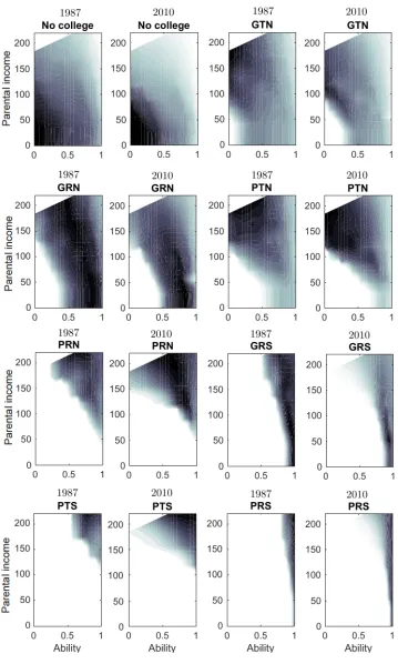
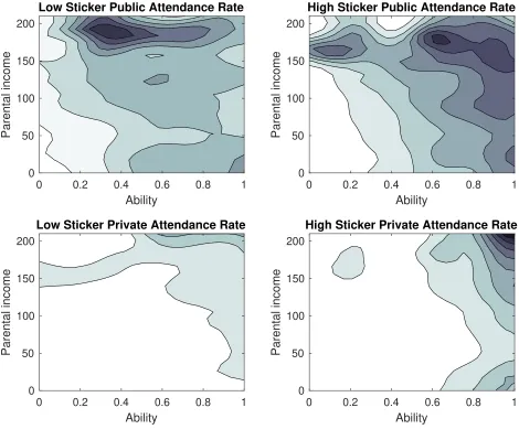
Regarding enrollment, the model replicates the 13 percentage point rise in the data—from 35%
to 48%—along with the fact that two-thirds of the increase accrues to public colleges. Delving into
the cross section, figure3shows heat maps for equilibrium enrollment in the model for both 1987 and 2010. The distributions of student abilities within each college type remain mostly stable, though
some interesting patterns emerge regarding the sorting of students by family resources. Specifically,
become more financially accessible because of greater tuition discounting.
While we cannot compare the enrollment patterns explicitly in 1987 and 2010 for want of data, we can use the NLSY97 to look at enrollment patterns around 2000. These are displayed
in figure 4 broken down into public verse private and high (i.e., above median) sticker versus low
(below median) sticker colleges. Evidently the sorting patterns in the model and data line up very closely. The highest ability and highest income students enroll at high sticker private schools (like
PRS). Students widely differing in ability attend public schools, with still some tendency towards
higher income (like GRN, GTN, and GRS). The lower price private schools cater mostly to affluent students (like PTS and PTN). Overall, the sorting of students across schools looks very reasonable
both in 1987 and 2010 when compared to attendance in the late 1990s and early 2000s.
4.3 What are the Most Important Tuition Drivers?
With the knowledge that the combined effect of all supply-side and demand-side forces is to cause
the model to replicate many of the trends in higher education from 1987 to 2010, we turn now to
quantifying the relative contribution of each factor in isolation. Table 6 gives the results of this decomposition exercise for enrollment-weighted net tuition. The first column under the net tuition
heading shows average equilibrium tuition in the model under several different scenarios, beginning
with a value of 5.8 (in thousands of 2010 dollars) from the calibration for 1987. All other values are untargeted.
When only Baumol’s cost disease is introduced, tuition rises from 5.8 to 6.2—an increase of $400.
The “Contribution” column scales this change in equilibrium tuition by the total actual change of 5.4 (= 11.2−5.8) observed in the data. Thus, Baumol’s cost disease explains approximately 0.4/5.4 = 7% of the total rise in net tuition from 1987 to 2010. Next up is the contribution of higher parental income and the increased expected return to college. Together, these factors inflate net tuition by over $4,000, which accounts for 76% of the total observed empirical change. Turning
to the remaining demand-side factor—the Bennett hypothesis—we find that shifts in financial aid
(mostly in the direction of greater generosity) account for 42% of the rise in tuition over this period. The next two rows shows the impact of movements in the non-tuition revenue received by colleges.
Given that both sources of endowment revenue have remained flat or gone up since 1987, they have
acted to restrain tuition growth, even if only modestly. Put another way, while it is true that state support for public institutions has declined as a percentage of college revenue, what matters for
equilibrium tuition is the absolute level of state support per student. With all forces present, the
last line confirms that the model matches (in fact, slightly overestimates by 8%) the overall rise in net tuition across all institutions.
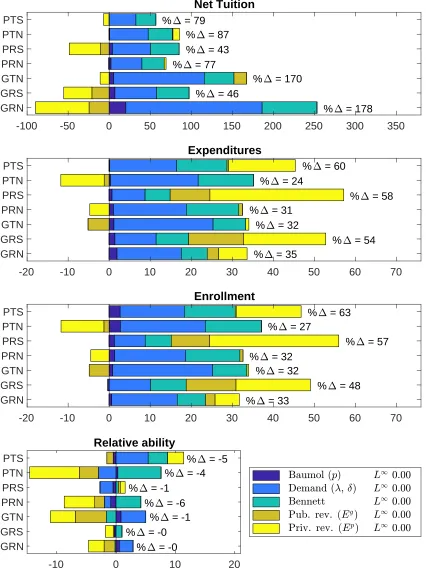
Figure 5 shows that underneath the aggregate decomposition lies substantial heterogeneity by college type.10 In this figure, each color represents the change induced by one factor in isolation,
Low Sticker Public Attendance Rate
0 0.2 0.4 0.6 0.8 1
Ability 0
50 100 150 200
Parental income
High Sticker Public Attendance Rate
0 0.2 0.4 0.6 0.8 1
Ability 0
50 100 150 200
Parental income
Low Sticker Private Attendance Rate
0 0.2 0.4 0.6 0.8 1
Ability 0
50 100 150 200
Parental income
High Sticker Private Attendance Rate
0 0.2 0.4 0.6 0.8 1
Ability 0
50 100 150 200
Parental income
Figure 4: Sorting patterns for attendance in the NLSY97
Net Tuition
Experiment Model Data Contribution (%)
1987 5.8 5.8 0
1987+Baumol’s Cost Disease (p) 6.2 - 7
1987+Labor Market Returns (δ,λ) 9.9 - 76
1987+Bennett Hypothesis 8.1 - 42
1987+State Support (Eg) 5.5 - -6
1987+Endowment Revenue (Ep) 4.6 - -23
2010 (1987+Everything) 11.6 11.2 108
Net Tuition
% = 178 % = 46
% = 170 % = 77
% = 43 % = 87 % = 79
-100 -50 0 50 100 150 200 250 300 350
GRN GRS GTN PRN PRS PTN PTS Expenditures
% = 35
% = 54 % = 32
% = 31
% = 58 % = 24
% = 60
-20 -10 0 10 20 30 40 50 60 70
GRN GRS GTN PRN PRS PTN PTS Enrollment
% = 33
% = 48 % = 32
% = 32
% = 57 % = 27
% = 63
-20 -10 0 10 20 30 40 50 60 70
GRN GRS GTN PRN PRS PTN PTS Relative ability
% = -0 % = -0
% = -1 % = -6 % = -1
% = -4 % = -5
-10 0 10 20
GRN GRS GTN PRN PRS PTN PTS
while “%∆” stands for the combined effect of all forces in the model. For example, equilibrium net
tuition increases by 79% for PTS (private teaching selective) colleges and 178% for GRN (govern-ment research non-selective) institutions. Continuing this comparison, the Bennett hypothesis and
all other demand-side factors contribute almost equally to higher tuition at PTS colleges, whereas
the Bennett hypothesis is relatively weaker at GRN colleges. Furthermore, changes in non-tuition revenue actually prevent tuition from going even higher at GRN schools but are not important for
explaining tuition inflation at PTS institutions. Figure5also reveals that the Bennett hypothesis—
far from being a story that only applies to elite colleges—actually has the biggest impact on tuition for GRN schools.
Turning to other variables, it is apparent that higher endowment revenue is a significant driver
of both increased expenditures and larger enrollment at selective institutions (whether public or private) but not elsewhere. By contrast, parental income and the rising returns to college are more
salient for expenditures and enrollment at non-selective colleges. When it comes to the Bennett
hypothesis, figure 5 indicates that expenditures and enrollment are more sensitive to financial aid at private colleges with the key exception of PRS (private research selective) institutions, which
tend to have significantly larger revenue streams from their endowments.
Lastly, although average student quality within each institution type remains relatively stable in the model (and data) between 1987 and 2010, individual supply-side and demand-side forces can
induce significant shifts in sorting by ability. For example, the “Relative ability” portion of figure
5 shows that, in isolation, higher endowment revenue increases enrollment by drawing students
from further down the ability distribution. In short, the average academic ability of the student
body at non-selective institutions would decline significantly if the only force at play were the rise in endowment revenue. By contrast, the increased availability of financial aid draws higher ability
students into attendance at private colleges while having almost no effect for public colleges.
4.4 Intuition from a special case
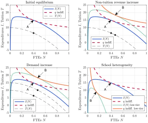
To develop some intuition, suppose thatq does not depend on X orY and consider partial equi-librium where the market tightnesses θ are fixed. Then consider a two-stage problem where a college first decides how many students to admit N and second decides which students to admit. Out of the second stage problem—which simply chooses vacancy posting to maximize the aver-age net tuition—comes an implied value T(N) and quality enhancing expenditures per student
I(N) = −C(N)/N + (T(N) + ¯Eg + ¯Ep)/p. Under the previous assumptions, T(N) is necessarily decreasing. Now consider how I(N) varies in N for the most attractive school. I(0) will be “nega-tive infinite” because of the fixed cost. As N increases, I first rises because the average total cost is decreasing. However, at some point I(N) attains a peak and begins to decrease because T(N) is decreasing and marginal custodial costs begin to rise. Hence, the graph of I(N) in figure 6 is
typical, to which we have added indifference curves of the quality function such that the optimal
choice is initially at the point labeledA.
A A
B
A
B
A
B
Figure 6: Tuition supply and demand curves in a simple example
Now, consider what happens if ¯Eg or ¯Ep increases as illustrated in the top right panel. The
I(N) curve shifts up uniformly to the green-dotted line. This creates a positive income effect that moves the college from point A to B, increasing both N∗ and I∗ (using ∗ to denote an optimal choice). Note that becauseT(N) is decreasing, this means net tuition T∗ must fall.
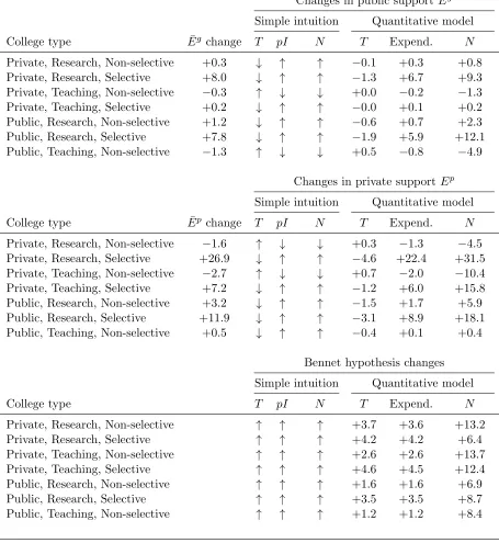
How does the prediction of increases in non-tuition revenue causing increases in enrollment and expenditures and falls in net tuition accord with the quantitative model? Table7 shows it accords
perfectly for all seven school types. In particular, whether the schools had increases or decreases
Changes in public supportEg
Simple intuition Quantitative model
College type E¯g change T pI N T Expend. N
Private, Research, Non-selective +0.3 ↓ ↑ ↑ −0.1 +0.3 +0.8
Private, Research, Selective +8.0 ↓ ↑ ↑ −1.3 +6.7 +9.3
Private, Teaching, Non-selective −0.3 ↑ ↓ ↓ +0.0 −0.2 −1.3
Private, Teaching, Selective +0.2 ↓ ↑ ↑ −0.0 +0.1 +0.2
Public, Research, Non-selective +1.2 ↓ ↑ ↑ −0.6 +0.7 +2.3
Public, Research, Selective +7.8 ↓ ↑ ↑ −1.9 +5.9 +12.1
Public, Teaching, Non-selective −1.3 ↑ ↓ ↓ +0.5 −0.8 −4.9
Changes in private supportEp
Simple intuition Quantitative model
College type E¯p change T pI N T Expend. N
Private, Research, Non-selective −1.6 ↑ ↓ ↓ +0.3 −1.3 −4.5 Private, Research, Selective +26.9 ↓ ↑ ↑ −4.6 +22.4 +31.5 Private, Teaching, Non-selective −2.7 ↑ ↓ ↓ +0.7 −2.0 −10.4 Private, Teaching, Selective +7.2 ↓ ↑ ↑ −1.2 +6.0 +15.8 Public, Research, Non-selective +3.2 ↓ ↑ ↑ −1.5 +1.7 +5.9 Public, Research, Selective +11.9 ↓ ↑ ↑ −3.1 +8.9 +18.1 Public, Teaching, Non-selective +0.5 ↓ ↑ ↑ −0.4 +0.1 +0.4
Bennet hypothesis changes
Simple intuition Quantitative model
College type T pI N T Expend. N
Private, Research, Non-selective ↑ ↑ ↑ +3.7 +3.6 +13.2
Private, Research, Selective ↑ ↑ ↑ +4.2 +4.2 +6.4
Private, Teaching, Non-selective ↑ ↑ ↑ +2.6 +2.6 +13.7
Private, Teaching, Selective ↑ ↑ ↑ +4.6 +4.5 +12.4
Public, Research, Non-selective ↑ ↑ ↑ +1.6 +1.6 +6.9
Public, Research, Selective ↑ ↑ ↑ +3.5 +3.5 +8.7
Public, Teaching, Non-selective ↑ ↑ ↑ +1.2 +1.2 +8.4
Note: financial variables are in thousands of 2010 dollars; enrollments are percent change from 1987 values.
When it comes to a demand increase, the effects are similar in that the I(N) curve, which creates a positive income effect. However, depending on precisely howT(N) changes, there may be a substitution effect as well. Supposing the demand change causesT(N) to increase uniformly, say by λ, againN∗ and I∗ will increase. But note that whileI∗ increases, it increases by less than λ. Consequently, T∗ goes up, but by less thanλso that rents are not fully extracted by the college.
The bottom panel of table 7 compares the quantitative model predictions for the Bennet
hy-pothesis changes with the intuition from the simple model. (Because the non-policy induced demand
changes are similar to Bennet, we omit them.) Again, all of the signs are as predicted.
Turning to the last experiment, Baumol cost disease creates a negative income effect in that
I(N) decreases, but it also creates a substitution effect in thatI(N) decreases proportionally more where the average total custodial cost is smaller or whereT(N)/pdecreases the most. Because the custodial costs are calibrated to be quite small, theT(N)/peffect tends to dominate, which make
I(N) curve flatter in addition to shifting it down. The substitution effect tends to increaseN and lower I, while the income effect tends to decrease both. The end result is that I∗ should decrease, with ambiguous effects on N∗, pI∗, and T∗ =T(N∗). Hence, the small and sometimes ambiguous effects (such as for enrollment) that Baumol cost disease produces in the quantitative model can
also be rationalized by the simple model.
Why does the intuition from a partial equilibrium formulation give such accurate predictions?
In part because the college market is extremely segmented. The highest tier schools essentially get the first pick of students, followed by the second highest tier, and so on. If a lower-tier school
wanted to enroll the highest ability students, it would need to spend inordinate amounts of money—
compensating the student for the net present value of income gains associated with going to an elite school—in the form of negative net tuition perhaps in excess of negative one million dollars.
Effectively, then, T(·) is mildly decreasing until it starts to fall drastically at some point (except at elite schools). This makes the I(N) curve peaked in a range ofN, as illustrated in the bottom right panel of figure6, that is mostly independent of what other schools are doing.
While we have worked through the results for where q does not depend onX orY, something similar can be done if q does not depend on N or Y. In particular, one can setup a two-stage problem where X is chosen first followed by implementing it in the second stage via admission of students. However, the second stage problem no longer reduces to just maximize average net
tuition but instead involves complicated tradeoffs. Still, the second stage delivers an expenditure curveI(X) and tuition curveT(X). Broadly speaking, the curves will be humpshaped, looking like in figure6whereN on the horizontal axis is replaced byX.11By the same logic as above, increases inEg,Ep and demand will drive upI∗ andX∗. Why then does average ability change little or even 11In particular, because of fixed costs, I(X) goes to negative infinity as X goes to 1. On the other hand, at
go in the opposite direction depending on the experiment? In large part it is because of the extreme
market segmentation mentioned above. This segmentation makes the humps very steep and puts
I∗ and X∗ close (but just to the right) of the peak. Consequently, when a positive income effect drives up theI(X) curve, increasingX∗ by any substantial amount is very costly, and it is cheaper (in quality terms) to increase I∗ a lot and only increase X∗ a little. Adding the dependence of q
on N, then, can easily overcome this tendency to increaseX∗ slightly with a desire to increase N∗
instead.
4.5 What Does a Taste for Enrollments Mean?
The previous section showed that a simplified setup where q depends only on I and N accurately predicts how tuition, expenditures, and enrollment change in response to non-tuition revenue and
demand changes. Before closing, it is worthwhile to interpret what a taste for enrollments actually means. For this, consider the Cobb-Douglas case of = 1, and maintain the assumption that q
does not depend on X or Y. Then q = IαINαN, which can be normalized to q = IαIN1−αI. If
αI = 1, then the indifference curves in figure 6 are horizontal. In this case, the optimal choice has
I0(N) = 0, which implies
T0(N) =pdC(N)/N dN .
Hence, the college admits student up to the point where the marginal average tuition revenue equals the marginal average custodial cost. Importantly, note that non-tuition revenue changes
in this case have no effect on tuition or enrollment (but rather show up as one-for-one increases
in expenditures). From a price equals marginal cost perspective, this is quite a surprising result, which highlights the difference between marginal cost (which here has essentially no relation with
tuition) and effective marginal cost (which has a strong, in fact perfect forκ= 0, relationship). This prediction stands in contrast to a large empirical literature that finds a negative relationship between non-tuition revenue (usually state support) and tuition. It also means that increases in demand
do not necessarily increase enrollments. For instance, absent student heterogeneity,T0(N) = 0 and hence enrollments are entirely determined by the minimum of the average cost function. Again, this seems at odds with the empirical literature which finds enrollment changes due to, e.g., changes in
public support.
On the other hand, now suppose αI = 1/2 so that college preferences can be represented by
q = (IN)1/2 or, equivalently, q = IN. In this case, colleges maximize total quality-enhancing expenditures instead of average expenditures. The quality indifference curve slope, which equals
−I/N in this case, must be equated toI0(N) as in figure 6. One can then show
T(N) = 1 1 +εT,N
pC(N)
N (1 +εNC,N)
−E¯g−E¯p
whereεf,x is the elasticity off with respect tox.12In this case, average net tuition must equal the
average custodial cost, adjusted by the elasticity εC/N,N, less non-tuition revenue plus a markup 1
1+εT ,N−1≥0. (And this markup is exactly what comes out of a typical monopolist or monopolistic
competition type problem.) Now changes in marginal costs, such as changes in marginal non-tuition
revenue, play a key role in determining the equilibrium level of net tuition. This specification has the potential to be consistent with the empirical literature finding that cuts in state support increase
tuition. It also implies increases in demand that drive up average net tuition T uniformly increase enrollments (as in the bottom left panel of figure6), again potentially consistent with the empirical literature.
Consequently, the taste for enrollments determines what price setting looks like. In the Epple
et al. (2006) framework where q does not depend on N, the equilibrium relates marginal average tuition with marginal average cost. In contrast, with an equally weighted taste for N and I, the equilibrium looks more like a conventional profit-maximization framework where tuition prices are
equated with marginal costs—even though schools are non-profits. Our calibrated model finds a middle-ground that matches tuition, expenditures, and enrollment well both cross-sectionally and
longitudinally.
5
Conclusion
Many explanations have been proffered for the rise in college tuition over the past few decades,
ranging from Baumol’s cost disease to labor market shifts to financial aid changes, just to name a few. Ample empirical evidence points to the existence of all these channels—for example, the
labor market premium for college graduates has clearly gone up—but what is unclear absent a
structural analysis is the extent to which each one is responsible for tuition inflation. The analysis in this paper suggests that, collectively, these existing hypothesis are sufficient to explain the path
that U.S. higher education has taken since at least the late 1980s. In other words, the analysis in
this paper does not point to any urgent need for an entirely new theory of tuition inflation. More importantly, the framework in this paper also sheds light on which of these factors matters the most,
and it turns out the answer varies to some extent by institution type. In the aggregate, demand-side
forces—notably, changes in the return to college and policy-induced increases in financial aid—are the primary drivers of average tuition growth. However, in the cross-section, the return to college
matters much more for tuition at public institutions than at private colleges, while increases in
endowment income have actually restrained tuition growth, but only at research-intensive colleges. Going forward, many fruitful extensions emerge for future research. First, whereas this paper
12
In particular,−I(N)/N =−d(C(N)/N)/dN+T0(N)/porpI(N) +T0(N)N=pN d(C(N)/N)/dN. Substituting in the I(N) curve, one has −pC(N)/N +T(N) + ¯Eg+ ¯Ep+T0
(N)N =pd(C(N)/N)/dN or T(N) +T0(N)N = p(C(N)/N+N d(C(N)/N)/dN)−E¯g−E¯p. Usingεf,x =dlogf(x)/dlogx=f0(x)x/f(x), one then hasT(N)(1 + εT ,N) =pC(NN)(1 +εC