Yield variability prediction by remote sensing sensors with different spatial resolution**
Jitka Kumhálová1* and Štěpánka Matějková21Department of Machinery Utilisation, Faculty of Engineering, Czech University of Life Sciences, Prague, Kamýcká 129, 165 21 Prague 6 - Suchdol, Czech Republic
2Research Team – Agricultural Soil Science and Pedobiology, Crop Research Institute, Drnovská 507, 161 06 Prague, Czech Republic
Received August 15, 2016; accepted March 10, 2017
*Corresponding author e-mail: [email protected] [email protected]
**This work was supported by CULS Prague Internal grant Project No. 20163005 (31160/1313/313104), 2016-2017
A b s t r a c t. Currently, remote sensing sensors are very popular for crop monitoring and yield prediction. This paper describes how satellite images with moderate (Landsat satel-lite data) and very high (QuickBird and WorldView-2 satelsatel-lite data) spatial resolution, together with GreenSeeker hand held crop sensor, can be used to estimate yield and crop growth varia- bility. Winter barley (2007 and 2015) and winter wheat (2009 and 2011) were chosen because of cloud-free data availabi- lity in the same time period for experimental field from Landsat satellite images and QuickBird or WorldView-2 images. Very high spatial resolution images were resampled to worse spatial resolution. Normalised difference vegetation index was derived from each satellite image data sets and it was also measured with GreenSeeker handheld crop sensor for the year 2015 only. Results showed that each satellite image data set can be used for yield and plant variability estimation. Nevertheless, better results, in comparison with crop yield, were obtained for images acquired in later phenological phases, e.g. in 2007 – BBCH 59 – average correlation coefficient 0.856, and in 2011 – BBCH 59-0.784. GreenSeeker handheld crop sensor was not suitable for yield esti-mation due to different measuring method.
K e y w o r d s: satellite images, GreenSeeker handheld crop sensor, plant growth modelling, phenological phases, spectral index
INTRODUCTION
It is commonly known that crop yield depends on crop growth variability, which is related to multiple factors that can be time-independent (e.g. substrate, topography, soil type and depth) or time-dependent. Annually linked factors may include anomalies in planting, emergence, or
weath-er conditions. Seasonally linked factors can include plant diseases, weed development, severe climatic events or irri-gation system malfunctions (Bégué et al., 2008).
Topography is one of the main factors affecting crop variability and crop yield. Godwin and Miller (2003) said that topography was one of the most obvious causes of va- riation in field crops. Crop variability and crop yield can be affected by the distribution of water on the field. Crops pro -duce more stable yields with a stable water inputs (Schmidt and Persson, 2003), and water redistribution on a field can be modelled by several methods (Marques da Silva and Silva, 2006, Kumhálová and Moudrý, 2014).Topographic wetness index (TWI) is a commonly used algorithm for detecting the water distribution within the field (Kumhálová et al., 2014; Sørensen et al., 2006).
Crop growth and yield can be efficiently monitored using canopy reflectance (Scudiero et al., 2016). Canopy reflectance models have been used widely for investigat -ing the response of vegetation indices to the variation of a number of factors and for understanding the mechanisms of interaction among these factors (Daughtry et al., 2000; Vincini et al., 2014; 2015). Different types of sensors mea-suring the amount of reflected solar radiation, from low-cost multispectral to high-cost imaging spectrometers, from low spatial to high spatial resolution, and from ground-based to satellite are available (Hunt et al., 2013). Traditional satel- lite systems such as Landsat have been widely used for agricultural purposes over large areas. The benefit of this system is spectral resolution (over 7 spectral bands) and possibility of freely available remote sensing data (www. usgs.com). Nevertheless one of the disadvantages of these
satellite images is their coarse spatial resolution (Zhang and Pierce, 2013), i.e. for Landsat images 30 m, and 16 days the temporal resolution. The new generation of satel-lites, such as QuickBird (QB) and WorldView-2 (WV-2) (DigitalGlobe, Logmont, Colorado, USA), provide multi-spectral data in the visible to infrared spectra that can be extremely useful in precision agriculture because of their high spatial resolution, 0.6 m for QB and 2 m for WV-2 satellite images (Mulla, 2013). The temporal resolution of these systems is 1 to 3 days for WV-2 and 3-7 days for QB.
Galambošová (2016) stated that another possibility for canopy reflectance measurement is, for example, the use of devices such as N sensor, Crop Spec, Crop Circle ACS, OptRX, ISARIA or Greenseeker. The Greenseeker (GS) as a crop sensor can be in handheld form as well. The GS optical sensor employs a patented technology to measure crop reflectance and to calculate the Normalised Difference Vegetation Index (NDVI). It also predicts yield potential. Nevertheless, the GS sensor is marketed primarily as a bio-mass sensor, not as N-sensor (Sharma et al., 2015). NDVI spectral index (Rouse et al., 1974) is based on the absorp-tion difference of photosynthetically active tissues in the red and near-infrared wavelengths of the electromagnetic spectrum (Julien et al., 2011). NDVI derived from meas-urements of canopy reflectance have been widely used for in-season estimation of yield. NDVI is used for the evalu-ation of different crops for different purposes at different scales (Domínguez et al., 2015; Tornos et al., 2014).
According to the literature, remote sensing sensors are very popular for monitor crop growth and for yield predic-tion (Scudiero, 2016). Therefore, the main aim of this study was to assess the suitability of selected sensors and their spatial resolution for monitoring crop variability and yield.
MATERIALS AND METHODS
The experimental data for this study were obtained from an experimental field of 11.5 ha in Prague-Ruzyne (50°05’N; 14°17’30”E), Czech Republic, with a Haplic Luvisol soil. Conventional arable soil tillage technology and fixed crop rotation were used on this field. Yield was measured by a combine harvester equipped with the yield monitor LH 500 (LH Agro, Denmark). Detailed description of the yield measuring device can be found in Kumhálová et al. (2011). Experimental variograms of yield were com-puted by common procedures using an exponential model. The 2009 yield data were not measured because of a sudden failure of the yield monitor.
Total monthly precipitation and temperature data were provided by the Agro meteorology station at the Crop Research Institute in Prague-Ruzyne. Precipitation and temperature for observed years are provided in Table 1.
The topographic data was derived from LiDAR data kindly provided by the Czech office for surveying, map -ping and cadastre. Elevation data were interpolated by inverse distance weighting (IDW) in ArcGIS 10.1 to create the DEM. The slope model (SM) and flow accumulation model (FAM) were then derived from the DEM – D8 algorithm. TWI uses SM and FAM raster data as inputs, based on the idea that low-gradient areas will gather water (high TWI values), whereas steep convex areas will shed water (low TWI values). TWI values are non-dimension-al relative indices and vary by landscape type and DEM. Detailed description of the TWI can be found in Kumhálová et al. (2014).
Winter barley (2007 and 2015) and winter wheat (2009 and 2011) were chosen because of cloud-free data availa- bility in the same period for the experimental field from Landsat satellite images and QuickBird or WorldView-2 images. Landsat satellite images were downloaded from the USGS Global Visualisation Viewer ( http://earthex-plorer.usgs.gov/). WV-2 and QB satellite images were purchased from the ArcDATA Company (Table 2). For atmospheric correction, the Fast Line-of-sight Atmospheric Analysis of Hypercubes was used (Dominguez et al., 2015; Li et al., 2014). All image pre-processing was implemented with ENVI SW (ENVI; version 5.3, Excelis, Inc., McLean, VA, USA).
NDVI values, as the ratio of reflectance in near infrared (NIR) and RED visible region (Rouse et al., 1974), were computed for every image with ENVI SW. The informa-tion about the range of wavelengths, satellite images, sensors and crops used in this study is provided in Table 2. T a b l e 1. Precipitations and temperatures in different growth
stages by BBCH scale recorded on the experimental field in selected years
Growth stage Winter barley Winter wheat
2007 2015 2009 2011
Precipitation (mm)
BBCH 20-29 122.4 81.2 184.2 104.4
BBCH 30-59 2.4 43.7 109.2 39.5
After BBCH 60 146.6 64.6 154.6 257.4
Sum 271.4 189.5 448.0 401.3
Mean 90.5 63.2 149.3 133.8
Temperature (°C)
BBCH 20-29 6.9 3.3 4.4 3.4
BBCH 30-59 12.8 12.3 14.3 14.8
After BBCH 60 18.1 17.1 17.7 17.9
Sum – – – –
All images were then exported into ArcGIS SW (ArcGIS; version 10.3.1, Esri, Inc., Redlands, CA, USA) for fur-ther processing. Selected images (WV-2 and QB), yield and TWI raster were resampled by changing the cell size according to satellite image outputs to 30, 0.6, and 2 m, and then to 4 m according to average measured yield point (ca. 16 m2) and 15 m as a control of spatial resolution. The
number of pixels used for evaluation was different for each of the evaluated years. It was caused by the fact that experi-mental plot boundary changed slightly between the years because of management practices. Only the pixels com-pletely inside the boundaries were used for the evaluation.
GreenSeeker (version 1.00, Rev B, 2012, Trimble Navigation Limited, USA) uses the red (660 nm, ~25 nm FWHM) and infrared (780 nm, ~25 nm FWHM) bands and converts reflected data into NDVI directly (Trimble, 2017). NDVI values from Greenseeker handheld crop sensor were collected during the winter barley growth on April 23rd, and May 19th2015. Experimental variograms of NDVI values were computed by common procedures using an exponential and spherical model.
Pearson correlations between the yield maps, TWI and NDVI derived from satellite images and GreenSeeker sen-sor were calculated using Statistica 13 (StatSoft Inc., Tulsa, USA) procedure.
RESULTS AND DISCUSSION
Correlation coefficients (R) between NDVI (from original and resampled data sets of Landsat, QB and WV-2 satellite images with different spatial resolution), TWI and yield were calculated for individual image data and plant species (Table 3). Summary statistics of crop yield and GS for selected dates and years are given in Table 4. Summary statistics for NDVI calculated from original and resampled satellite images for selected crops are in Table 5.
Correlation matrices between NDVI from GS crop sensor, Landsat satellite images, yield and TWI were then calcu-lated for individual data sets of winter barley (Table 6).
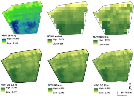
Winter barley was grown in 2007 and 2015. In 2007, yield and TWI had higher R (0.433 for SR of Landsat and 0.530 for QB) (Table 3). That year was drier in comparison with other years (Table 1). Low precipitation (2.4 mm) in the growth stage BBCH 30-59 can cause a significant dis -placement of relatively higher yield to water-accumulating depressions. This fact is confirmed also by correlations pre -sented in Table 3, where R between NDVI and yield had average value of 0.856 and R between TWI and NDVI had average value of 0.419 for all spatial resolutions (Fig. 1). The movement of higher yield to concave areas in 2007 was also validated by summary statistics presented in Table 4, whereby both standard deviation and min-max range were higher than in 2015. In our previous articles (Kumhálová et al., 2011; 2014), the influence of topography on yield in
drier years was also found. Table 5 and Fig. 2 show that the NDVI values depended on the sensor used.
In 2015, winter barley yield and TWI had lower Rva- lues (0.242 for Landsat and 0.148 for WV-2) (Table 3). The year 2015 was the driest among the years analysed in our study. The precipitation distribution was uneven during the winter barley growth (in BBCH 20-29, 81.2 mm only). On the contrary, the precipitation distribution in BBCH 30-59 (43.7 mm) could probably cause the later crop to be beaten. In that year, harvesting losses caused by crop beat-ing decreased the yield. This fact was confirmed by low R values between yield and NDVI (Table 3), although the NDVI values were relatively high during BBCH 21-22 and crops were in a good condition (Table 5). Winter wheat was grown in 2009 and 2011. Unfortunately, in the year 2009 the yield was not measured. Table 3 shows that the R between TWI and NDVI from QB was very weak. It corre-sponds with more precipitation distribution (Table 1) on the date of satellite data acquisition. The differences between
T a b l e 2. Available satellite images for the selected years
Satellite Sensor RED range NIR range Date Crop Growth stage
nm
Landsat 5 TM 630-690 760-900 24 May 2007 winter barley BBCH 59
Landsat 7 ETM+ 630-690 750-900 19 April 2009 winter wheat BBCH 20-29
26 May 2011 winter wheat BBCH 59
Landsat 8 OLI 640-670 850-880 18 March 2015 winter barley BBCH 21-22
QuickBird
590-710 715-918 22 May 2007 winter barley BBCH 59 13 April 2009 winter wheat BBCH 20-29 31 May 2011 winter wheat BBCH 59
sensors response can be seen between NDVI from Landsat and QB in Tables 3 and 5 as well. Landsat images showed noticeably higher values in all cases than the QB images in each spatial resolution.
In the year 2011, Table 3 shows higher R between win-ter wheat yield and TWI (0.498 for Landsat and 0.630 for QB). The precipitation distribution was uneven during the winter wheat growth (after BBCH 60 - 257.4 mm) (Table 1). Correlation coefficients between yield and TWI reached high values (Table 3). This crop response was probably caused by low precipitation during the growth stages BBCH 30-59. Again, low precipitation can cause a significant dis -placement of relatively higher yield to water-accumulating depressions (Kumhálová et al., 2011; 2014). The sum-mary statistics presented in Table 4 confirmed again the
yield inequality. On the contrary, the summary statistics of NDVI presented in Table 5 showed similar values obtained by sensors used in this study.
GS measurements on April 23rd (BBCH 31) and May 19th (BBCH 55), 2015, and comparisons between NDVI from GS and Landsat images, yield and TWI in Table 6 are in good accordance with previous statements about crop development during the year 2015. Nevertheless, R between NDVI from GS and Landsat images were weak. It could be caused by the different method of data collection.
NDVI derived from Landsat and QB data showed similar results for later sensing (BBCH 59). For early sens-ing stage (BBCH 20-29), significant differences between the results from Landsat and QB were found (Table 3). It could be influenced by the soil sensing between the crops.
T a b l e 3. Correlation coefficients between normalised difference vegetation index (NDVI) (from original and resampled Landsat (L), QuickBird (QB) and WorldView-2 (WV-2) satellite images with different spatial resolution (SR)), topographic wetness index (TWI) and resampled yield (to different SR) of selected crops and years
Parameter Yield NDVI
Winter barley 2007
Satellite L 5 TM QB L-5 QB QB QB QB
SR (m) 30 0.6 30 0.6 4 15 30
Yield 1 1 0.861*** 0.861*** 0.859*** 0.865*** 0.835***
TWI 0.433*** 0.530*** 0.485*** 0.427*** 0.428*** 0.444*** 0.313***
2015
Satellite L 8 OLI WV-2 L-8 WV-2 WV-2 WV-2 WV-2
SR (m) 30 2 30 2 4 15 30
Yield 1 1 0.264** 0.133*** 0.134*** 0.119** -0.018
TWI 0.242* 0.148*** 0.360*** -0.030*** -0.045*** 0.158*** -0.055
Winter wheat 2009
Satellite L 7 ETM+ QB L-7 QB QB QB QB
SR (m) 30 0.6 30 0.6 4 15 30
TWI – – 0.495*** -0.033*** -0.026* -0.041 0.109
2011
Satellite L 7 ETM+ QB L-7 QB QB QB QB
Yield 1 1 0.821*** 0.785*** 0.781*** 0.792*** 0.739***
TWI 0.498*** 0.630*** 0.515*** 0.397*** 0.393*** 0.409*** 0.250*
Domínguezet al. (2015) discussed in their study how the phenological phase of the crop could influence the NDVI values during the crop growth. They developed NDVI mo- dels for winter wheat and winter rape crops from seeding to later phenological phases of selected crops. The results of our study are in accordance with the study of Domínguez et al. (2015). Scudiero (2016) noted that more research is needed to define, by geographical region, which sensor measurements are most useful for improving soil and crop management. Images resampled to different spatial resolu-tions showed similar mean but decreasing min-max range with decreasing spatial resolution. This fact was confirmed for each year studied. The spatial resolution of images used in this study did not play any crucial role for yield variabi- lity prediction. It could be an important property for crop evaluation in a small scale, for example for weed detection (Wu et al., 2011). Based on our results, the GS device is not suitable for yield estimation. This is in contrary with Walsh et al. (2013). They noted that GS NDVI was a better pre-dictor of final winter wheat yield in a dry site-year. On the other hand, Updike and Comp (2010) stated that many of the differences in analysis of results can be explained by the differences in the sensors themselves. Vincini et al. (2015) discussed that experimental datasets can be affected by experimental error, due for example to imperfect sampling. It corresponds with the study of Ciganda et al. (2012). Those authors determined the number of leaf layers sensed by red-edge chlorophyll index. They found that vertical distribution of chlorophyll contents in leaves significantly influenced remote sensing techniques. Those techniques need to meet very stringent requirements for this reason.
Zhang (2016) also highlighted that some differences exist between sensor systems. These differences can be caused by the variations in bandwidth of the particular spectral chan-nels of the measuring systems. Mather and Koch (2011) described that one of the problems met in remote sensing is that the spectral reflectance of a given Earth-surface cover type is influenced by a variety of confusing factors. Casa et al. (2015) stated that small geometric registration errors typically do occur between the sensors used, even when an accurate calibration is performed.
CONCLUSIONS
1. On the basis of presented results it may be concluded that each satellite image data source used in this study can
sufficiently explain yield variability regardless to spatial
resolution of the images. Better results, in comparison with crop yield, were obtained for images acquired in later phe-nological phases. Images acquired in early phephe-nological phases showed differences according to sensor used. The sensors usually differ in bandwidth. Other reason of varia-tions can be early scanning of the crop (when soil is visible between the plants).
2. GreenSeeker handheld crop sensor is not suitable for yield estimation of the whole agriculture plot due to high workload of this procedure based on long time required for data collection and the necessity of using the interpolation method to obtain the map. In contrast, satellite image is acquired in a relatively very short time.
3. Results obtained in this study can be helpful for the selection of suitable sensor with adequate spatial resolution for yield estimation.
T a b l e 4. Summary statistics and method of interpolation used for plant yield (t ha-1) in selected years and for NDVI from GreenSeeker (GS) sensor
Parameter Winter barley Winter wheat GS
2007 2015 2011 23 April 2015 19 May 2015
Count 8808.0 10974.0 7548.0 103.0 103.0
Mean 5.618 5.322 7.053 0.779 0.802
Median 5.481 5.385 7.218 0.790 0.810
Standard deviation 1.373 0.836 1.953 0.062 0.030
Minimum 1.109 1.391 0.589 0.390 0.670
Maximum 10.149 9.254 13.458 0.890 0.850
Skewness 0.015 -0.666 -0.141 -2.946 -2.206
Method of interpolation Kriging
Method of estimation Method of moments (MoM)
Variogram model Exponential Spherical
Distance parameter (r) 22.9 11.0 45.3 205.7 610.9
Approximate range = 3 x r 68.7 33.0 135.9 617.1
-Nugget variance 0.3170 0.4200 1.3800 0.0025 0.0005
T a b l e 6. Correlation coefficients between normalised difference vegetation index (NDVI) from GreenSeeker (GS) sensor, Landsat images, crop yield and TWI of winter barley
2015 Date/SR (m) GS NDVI GS NDVI L-8 NDVI L-8 NDVI
Date April 23 May 19 April 19 May 14
Yield 30 0.011 0.022 0.260** 0.145
TWI 30 0.075 0.041 0.411*** 0.165
L8 NDVI April 19 0.310* – – –
L8 NDVI May 14 – 0.359*** – –
Levels of statistical significance: *p<0.05, **p<0.01, ***p<0.001.
T a b l e 5. Summary statistics for NDVI calculated from original and resampled satellite images for selected years and crops
Satellite L-5 QB L-8 WV-2
Parameter Winter barley
2007 2015
SR (m) 30 0.6 4 15 30 30 2 4 15 30
Count 115 306704 6880 485 115 102 26684 6627 469 102
Mean 0.756 0.635 0.636 0.635 0.635 0.528 0.414 0.414 0.414 0.418
Median 0.759 0.638 0.638 0.637 0.635 0.532 0.416 0.415 0.413 0.418
Standard
deviation 0.077 0.041 0.041 0.041 0.039 0.046 0.057 0.058 0.058 0.056
Minimum 0.556 0.477 0.490 0.495 0.544 0.315 0.185 0.191 0.219 0.269
Maximum 0.876 0.799 0.750 0.728 0.721 0.626 0.619 0.597 0.559 0.559
Skewness -0.664 -0.401 -0.408 -0.420 -0.138 -1.047 -0.153 -0.160 -0.242 -0.353
Satellite L-7 QB L-7 QB
Winter wheat
2009 2011
SR (m) 30 0.6 4 15 30 30 0.6 4 15 30
Count 107 300157 6722 482 107 101 293279 6562 464 101
Mean 0.774 0.591 0.591 0.591 0.583 0.800 0.773 0.774 0.773 0.775
Median 0.782 0.591 0.592 0.592 0.585 0.808 0.780 0.781 0.779 0.782
Standard
deviation 0.044 0.043 0.042 0.043 0.041 0.055 0.044 0.044 0.044 0.044
Minimum 0.492 0.301 0.305 0.333 0.325 0.616 0.550 0.580 0.607 0.616
Maximum 0.833 1.050 0.761 0.726 0.651 0.876 1.076 1.018 0.932 0.887
Fig. 1. Maps of kriged yield predictions in the experimental field during the observed years: a – 2007 – winter barley, b – 2011 – winter wheat, and c – topographic wetness index model map.
Conflict of interest: There is no conflict of interest which could influence the content of the article.
REFERENCES
Bégué A., Todoroff P., and Pater J., 2008. Multi-time scale ana- lysis of sugarcane within-field variability: improved crop diagnosis using satellite time series? Precision Agriculture, 9, 161-171.
Casa R., Castaldi F., Pascucci S., and Pignatti S., 2015. Chlorophyll estimation in field crops: an assessment of handheld leaf meters and spectral reflectance measure -ments. J. Agricultural Sci., 153, 876-890.
Ciganda V.S., Gitelson A.A., and Schepers J., 2012. How deep does a remote sensor sense? Expression of chlorophyll con-tent in a maize canopy. Remote Sensing Environment, 126, 240-247.
Daughtry C.S.T., Walthall C.L., Kim M.S., Brown de Colstoun E., and McMurtrey III J.E, 2000. Estimating corn leaf chlorophyll concentration from leaf and canopy reflectance. Remote Sensing Environ., 74(2), 229-239.
Dominguez J.A., Kumhálová J., and Novák P., 2015. Winter oilseed rape and winter wheat growth prediction using remote sensing methods. Plant Soil Environment, 61(9), 410-416.
Frogbrook Z.L., 1999. The effect of sampling intensity on the reliability of predictions and maps of soil properties. In: Precision Agriculture, Proc. 2nd European Conf. Precision Agriculture (Ed. J.V. Stafford). Sheffield Academic Press, Sheffield, UK.
Galambošová J., 2016. Remote sensing methods to determine crop parameters suitable for variable rate Nitrogen applica-tion on small grain cereals. Scientific Monograph, Research Institute of Agricultural Engineering, p.r.i., Prague, Czech Republic.
Godwin R.J. and Miller P.C.H., 2003. A review of the technolo-gies for mapping within-filed variability. Biosystems Eng., 84, 393-407.
Hunt Jr. E.R., Doraiswamy P.C., McMurtrey J.E., Daughtry C.S.T., Perry E.M., and Akhmedov B., 2013. A visible band index for remote sensing leaf chlorophyll content at the canopy scale. Int. J. Applied Earth Observation Geoinformation, 21, 103-112.
Julien Y., Sobrino J.A., and Jiménez-Muñoz J.-C., 2011. Land use classification from multitemporal Landsat imagery using the Yearly Land Cover Dynamics (YLCD) method. Int. J. Applied Earth Observation Geoinfor., 13, 711-720. Kumhálová J., Kumhála F., Kroulík M., and Matějková Š., 2011.
The impact of topography on soil properties and yield and the effects of weather conditions. Precision Agriculture, 12, 813-830.
Kumhálová J. and Moudrý V., 2014. Topographical characteris-tics for precision agriculture in conditions of the Czech Republic. Applied Geography, 50, 90-98.
Kumhálová J., Zemek F., Novák P., Brovkina O., and Mayerová M., 2014. Use of Landsat images for yield evaluation with-in a small plot. Plant Soil Environ., 60(11), 501-506. Li P., Jiang L., and Feng Z., 2014. Cross-comparison of
vegeta-tion indices derived from Landsat-7 enhanced thematic mapper plus (ETM+) and Landsat-8 operational land ima-ger (OLI) Sensors. Remote Sensing, 6, 310-329.
Marques da Silva J.R. and Silva L.L., 2006. Relationship between distance to flow accumulation lines and spatial variability of irrigated maize grain yield and moisture at harvest. Biosystems Eng., 94, 525-533.
Mather P.M. and Koch M., 2011. Computer processing of remotely sensed images: An introduction. Wiley Press, Chichester, UK.
Mulla D.J., 2013. Twenty five years of remote sensing in preci -sion agriculture: Key advances and remaining knowledge gaps. Biosystems Eng., 11, 358-371.
Rouse J.W., Haas R.H., Schell J.A., and Deering D.W., 1974. Monitoring vegetation systems in the Great Plains with ERTS. In: Proceedings Third ERTS-1 Symposium, NASA Goddard, NASA SP-351, 309-317.
Schmidt F. and Persson A., 2003. Comparison of DEM data cap-ture and topographic wetness indices. Precision Agriculcap-ture, 4, 179-192.
Scudiero E., Corwin D.L., Wienhold B.J., Bosley B., Shanahan J.F., and Johnson C.K., 2016. Downscaling Landsat 7 canopy reflectance employing a multi-soil sensor platform. Precision Agriculture, 17, 53-73.
Sharma L.K., Bu H., Denton A., and Franzen D.W., 2015. Active-optical sensors using red NDVI compared to red edge NDVI for prediction of corn grain yield in North Dakota, U.S.A. Sensors, 15, 27832-27853.
Sharma L.K. and Franzen D.W., 2014. Use of corn height to improve the relationship between active optical sensor readings and yield estimates. Precision Agriculture, 15, 331-345.
Sørensen R., Zinko U., and Seibert J., 2006. On the calculation of the topographic wetness index: evaluation of different methods based on field observations. Hydrology Earth System Sci., 10, 101-112.
Tornos L., Huesca M., Dominguez J.A., Moyano M.C., Cicuendez V., Recuero L., and Palacios-Orueta A., 2014. Assessment of MODIS spectral indices for determining rice paddy agricultural practices and hydroperiod. ISPRS J. Photogrammetry Remote Sensing, 101, 110-124.
Trimble, 2017. GreenSeeker handheld crop sensor. Trimble Inc., online: http://www.trimble.com/Agriculture/gs-handheld. aspx?tab=Product_Overview (accessed 20.1.2017). Updike T. and Comp Ch., 2010. Radiometric Use of WorldView-2
Imagery. Technical Note. DigitalGlobe, Inc.
Vincini M., Amaducci S., and Frazzi E., 2014. Empirical esti-mation of leaf chlorophyll density in winter wheat canopies using Sentinel-2 spectral resolution. IEEE Trans. Geoscience Remote Sensing, 52, 3220-3235.
Vincini M., Calegari F., and Casa R., 2015. Sensitivity of leaf chlorophyll empirical estimators obtained at Senstinel-2 spectra resolution for different canopy structures. Precision Agriculture, 17, 313-331.
Walsh O.S., Klatt A.R., Solie J.B., Godsey C.B., and Raun W.R., 2013. Use of soil moisture data for refined GreenSeeker sensor based nitrogen recommendations in winter wheat (Triticum aestivum L.). Precision Agriculture, 14, 343-356.
Wu X., Xu W., Song Y., and Cai M., 2011. A detection method of weed in wheat field on machine vision. Procedia Eng., 15, 1998-2003.
Zhang Q., 2016. Precision agriculture technology for crop farm-ing. CRC Press. Boca Raton, London, New York.